Structure [fdip-008R]
✍️sourceAGENTDRAFTED
- November 3, 2026
Structure [fdip-008R]
✍️sourceAGENTDRAFTED
- November 3, 2026
Can the physics be rebuilt from its observables alone? What replaces calculus when space is discrete?
The chapters below develop these questions. What the structure fixes and what it leaves free records what they fix and what remains an additional input.
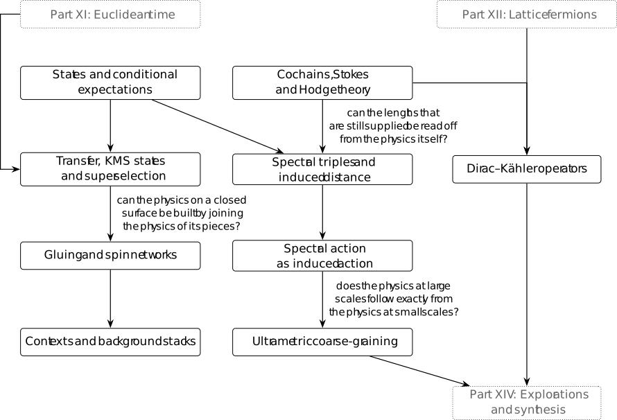
The arrows from Euclidean time enter the transfer chapter; those from lattice fermions enter the Dirac-Kähler chapter. They mark selected intended prerequisites for the chapters below, while the two opening questions motivate the part as a whole. Other suppliers are specified when each construction is developed.
1. States and conditional expectations [fdip-008S]AGENTDRAFTED
- November 2, 2026
1. States and conditional expectations [fdip-008S]AGENTDRAFTED
- November 2, 2026
Can the physics be rebuilt from its observables alone? This chapter asks how a state on a finite-dimensional algebra determines a Hilbert space.
The first section builds that space from the Gram form \(\omega (a^*b)\). Its dimension is the rank of the Gram matrix. On a direct sum of matrix algebras that rank is the sum of each block size times the rank of the density, and on functions the space is \(\ell ^2\) of the support. No norm on the algebra is assumed. The following section shows that a Wick conditional expectation sends polynomials to polynomials in the retained variables and that nested retained sets compose. The normalized Grassmann state restricts to the state of the Schur complement.
Theorem 1.1. Finite *-algebras, states and GNS [fdip-008T]AGENTDRAFTED
- November 2, 2026
Theorem 1.1. Finite *-algebras, states and GNS [fdip-008T]AGENTDRAFTED
- November 2, 2026
A state in the sense of the real and complex algebraic states is a normalized positive functional. That note assumes no norm and no operator representation. On a finite-dimensional *-algebra the functional itself determines both. The squared length of a class is the value of the state on \(\,a^*a\), and the dimension of the resulting space is the rank of one Gram matrix.
Let \(K=\mathbb R\) or \(K=\mathbb C\), and let \(A\) be a finite-dimensional unital associative \(K\)-algebra with an involution of the kind fixed for a real algebraic state or a complex algebraic state. Let \(\omega \) be a real or complex algebraic state on \(A\), according to the scalar field: \(K\)-linear, normalized in the sense of a normalized linear functional, Hermitian positive, and satisfying \(\omega (a^*a)\ge 0\). Define \(\langle x,y\rangle =\omega (x^*y)\). Let \(N\) be the set of \(x\) with \(\langle x,x\rangle =0\). The quotient \(H_\omega =A/N\) carries the descended inner product, the operator \(\pi _\omega (a)\) sends the class of \(b\) to the class of \(ab\), and \(\Omega \) is the class of \(1\).
The form is positive semidefinite and Hermitian, and \(N\) is a left ideal. For the cyclic vector, \[\langle \pi _\omega (a)\Omega ,\pi _\omega (b)\Omega \rangle =\omega (a^*b).\] For any basis the Gram matrix \(G_{ij}=\omega (e_i^*e_j)\) has \(\dim H_\omega =\operatorname {rank} G\). The squared length of the class of \(a\) is \(\omega (a^*a)\).
Let \(A=\bigoplus _i M_{m_i}(K)\), with componentwise product and with conjugate transpose acting on each block. Suppose each \(\rho _i\) has the form \(\rho _i=c_i^*c_i\), and \(\sum _i\mathrm {Tr}(\rho _i)=1\). The functional \(\omega (a)=\sum _i\mathrm {Tr}(\rho _i a_i)\) is a state, and \[\dim H_\omega =\sum _i m_i\operatorname {rank}\rho _i.\] On \(M_2\), the density \(\mathrm {diag}(2/3,1/3)\) has rank \(2\) and gives dimension \(4\). The density \(\mathrm {diag}(1,0)\) has rank \(1\) and gives dimension \(2\).
Let \(X\) be a finite set and let \(A\) be the algebra of functions \(X\to K\), with pointwise product and pointwise conjugation. Let \(w:X\to \mathbb R_{\geq 0}\) satisfy \(\sum _x w(x)=1\), and set \(\omega (f)=\sum _x w(x)f(x)\). Write \(\operatorname {supp} w\) for the labels with \(w(x)>0\). Then \(H_\omega \) is the space of all functions on that support, with the inner product weighted by \(w\). On a finite set that space is \(\ell ^2(\operatorname {supp} w)\).
Equivariant precision and real types records, inside a symmetry sector, a matrix over the reals, the complexes or the quaternions. This section does not prove that those matrices are the blocks of a decomposition of the observable algebra.
Proof.
- November 2, 2026
Proof.
- November 2, 2026
The form is linear in the second argument because \(\omega \) is.
It is conjugate-linear in the first because \((\lambda x)^*=\overline \lambda \,x^*\).
It is Hermitian because \(\langle y,x\rangle \) equals \(\omega ((x^*y)^*)\), and Hermitian positivity makes that the conjugate of \(\omega (x^*y)\). The square \(\langle x,x\rangle =\omega (x^*x)\) is nonnegative by the state.
The inequality of Cauchy and Schwarz is \(\lvert \langle x,y\rangle \rvert ^2\le \langle x,x\rangle \langle y,y\rangle \). Over \(\mathbb C\), if \(\langle x,y\rangle \) is not zero, choose a scalar \(u\) of modulus \(1\) with \(u\langle x,y\rangle =\lvert \langle x,y\rangle \rvert \), and replace \(y\) by \(uy\). The new square \(\langle y,y\rangle \) is unchanged, and the new inner product is real and nonnegative. Over \(\mathbb R\) no phase is required. For every real \(t\), \[\langle x+ty,x+ty\rangle =\langle x,x\rangle +2t\langle x,y\rangle +t^2\langle y,y\rangle \ge 0.\] If \(\langle y,y\rangle =0\), the values \(2t\langle x,y\rangle \) cannot stay above \(- \langle x,x\rangle \) for every real \(t\) unless \(\langle x,y\rangle =0\). If \(\langle y,y\rangle >0\), complete the square. The same quadratic is \[\langle y,y\rangle \Bigl (t+\frac {\langle x,y\rangle }{\langle y,y\rangle }\Bigr )^2 +\langle x,x\rangle -\frac {\langle x,y\rangle ^2}{\langle y,y\rangle }.\] The squared term can be made zero, so the remaining term is nonnegative. Thus the inequality holds. Over \(\mathbb C\), putting the unimodular factor back into \(y\) multiplies \(\langle x,y\rangle \) by a scalar of modulus \(1\) and does not change \(\langle y,y\rangle \).
If \(\langle x,x\rangle =0\), the inequality forces \(\langle x,y\rangle =0\) for every \(y\). Conversely the case \(y=x\) shows that the radical is exactly \(N\). It is a subspace. If \(x,y\in N\) and \(\lambda \in K\), then \[\begin {aligned} \langle x+\lambda y,x+\lambda y\rangle ={}&\langle x,x\rangle +\lambda \langle x,y\rangle \\ &+\overline {\lambda }\langle y,x\rangle +\lvert \lambda \rvert ^2\langle y,y\rangle . \end {aligned}\] The two squares vanish because \(x,y\in N\). The two cross terms vanish because an element of \(N\) is orthogonal to every vector. It is a left ideal. For \(b\in A\) and \(x\in N\), \(\langle bx,bx\rangle =\omega (x^*b^*bx)=\langle x,(b^*b)x\rangle =0\).
The form therefore descends to the quotient. If \(x-x'\) and \(y-y'\) lie in \(N\), then \(\langle x,y\rangle -\langle x',y'\rangle =\langle x-x',y\rangle +\langle x',y-y'\rangle \). The first summand vanishes because \(x-x'\) is in the radical. The second is the conjugate of \(\langle y-y',x'\rangle \), which vanishes for the same reason. The descended form is positive definite, and finite dimensionality makes the quotient a Hilbert space with no further completion. Its dimension is \(\dim A-\dim N\).
On a basis \(e_1,\ldots ,e_n\), the matrix \(G_{ij}=\langle e_i,e_j\rangle =\omega (e_i^*e_j)\) is Hermitian. A vector \(v\) represents \(x=\sum _i v_i e_i\). Hermitian symmetry gives \(G_{ji}=\overline {G_{ij}}\). The number \(\langle x,e_j\rangle =\sum _i\overline {v_i}G_{ij}\) vanishes for every \(j\) if and only if \(x\in N\): the forward direction was proved for every vector, and the converse is linearity in the second argument. Conjugating those sums and replacing \(\overline {G_{ij}}\) by \(G_{ji}\) produces \((Gv)_j=0\). Rank-nullity gives \(\operatorname {rank} G=n-\dim N=\dim H_\omega \). The class of \(a\) has squared length \(\omega (a^*a)\). The operator \(\pi _\omega (a)\) is well defined because \(N\) is a left ideal, and \(\langle \pi _\omega (a)\Omega ,\pi _\omega (b)\Omega \rangle =\langle a,b\rangle =\omega (a^*b)\).
On the direct sum, the product and the involution act blockwise, so \(\omega (a^*a)=\sum _i\mathrm {Tr}(\rho _i a_i^*a_i)\). The trace is invariant under a cyclic permutation, and \(\mathrm {Tr}(b^*b)\) is the sum of the squared moduli of the entries of \(b\). Hence \[\mathrm {Tr}(\rho _i a_i^*a_i) =\mathrm {Tr}(c_i a_i^*a_i c_i^*) =\mathrm {Tr}\bigl ((a_i c_i^*)^*(a_i c_i^*)\bigr ),\] which is nonnegative. The functional is therefore positive. It is normalized because \(\omega (1)=\sum _i\mathrm {Tr}(\rho _i)=1\). Each \(\rho _i=c_i^*c_i\) is self-adjoint. The trace of a conjugate transpose is the conjugate of the trace, and \((a_i\rho _i)^*=\rho _i a_i^*\), so \(\mathrm {Tr}(\rho _i a_i^*)=\overline {\mathrm {Tr}(\rho _i a_i)}\). Thus \(\omega \) is Hermitian.
The same identity shows that \(\omega (a^*a)=0\) if and only if \(a_i c_i^*=0\) for every \(i\). Different blocks occupy complementary summands, so \(\dim N=\sum _i\dim \{a_i:a_i c_i^*=0\}\). A matrix vanishes on a subspace precisely when it factors through the quotient by that subspace. The image of \(c_i^*\) has dimension \(\operatorname {rank} c_i^*\). The matrices vanishing on it are determined by their values on a complement, so their space has dimension \(m_i\bigl (m_i-\operatorname {rank} c_i^*\bigr )\). The quotient of that block therefore has dimension \(m_i\operatorname {rank} c_i^*\). Summing over the blocks gives \(\dim H_\omega =\sum _i m_i\operatorname {rank} c_i^*\).
It remains to match that rank with \(\operatorname {rank}\rho _i\). For the standard inner product, \(\|c_i v\|^2=\langle c_i^*c_i v,v\rangle \). If \(c_i^*c_i v=0\), the right-hand side vanishes, so \(c_i v=0\). The converse is immediate, and rank-nullity gives \(\operatorname {rank}\rho _i=\operatorname {rank} c_i\). A minor of a transpose is the transpose of a minor, and the determinant is unchanged by transposition. A minor of a conjugate transpose is the conjugate of a minor of the transpose. The largest size of a nonzero minor is therefore the same for \(c_i\), \(c_i^T\) and \(c_i^*\). Hence \(\operatorname {rank} c_i^*=\operatorname {rank}\rho _i\), and \(\dim H_\omega =\sum _i m_i\operatorname {rank}\rho _i\). On \(M_2\), \(\mathrm {diag}(2/3,1/3)\) is the square of \(\mathrm {diag}(\sqrt {2/3},\sqrt {1/3})\), so its rank is \(2\). \(\mathrm {diag}(1,0)\) is the square of \(\mathrm {diag}(1,0)\), and its only nonzero minor has size \(1\). The formula gives dimensions \(4\) and \(2\).
On functions, the indicator basis is orthogonal for the Gram form. Indeed \(\omega (1_x^*1_y)=\delta _{xy}w(x)\), so the Gram matrix is diagonal with entries \(w(x)\). Its rank is the number of strictly positive weights. A function lies in \(N\) exactly when it vanishes on \(\operatorname {supp} w\), because \(\omega (f^*f)=\sum _x w(x)\lvert f(x)\rvert ^2\). Two functions determine the same class exactly when they agree on that support, and every function on the support arises in this way. The descended inner product is \[\langle f,g\rangle =\sum _{w(x)>0}w(x)\overline {f(x)}\,g(x).\] Every function on a finite set is square-summable, so the space is \(\ell ^2(\operatorname {supp} w)\).
Theorem 1.2. Nested conditional expectations compose [fdip-008U]AGENTDRAFTED
- November 2, 2026
Theorem 1.2. Nested conditional expectations compose [fdip-008U]AGENTDRAFTED
- November 2, 2026
Let \(A\) be a unital associative algebra and \(\omega \) a linear functional on \(A\). Let \(B\subset A\) be a unital subalgebra. A conditional expectation of \(\omega \) onto \(B\) is a linear map \(E:A\to B\) with \(E(1)=1\), \(E(b_1ab_2)=b_1E(a)b_2\) for \(b_1,b_2\in B\), and \(\omega (E(a))=\omega (a)\). When \(A\) carries the involution of an algebraic state, \(\omega \) is such a state, and \(E(a^*)=E(a)^*\), the same identities give \(\omega (c^*E(a^*a)c)=\omega ((ac)^*(ac))\) for \(c\in B\). No norm on \(A\) enters that identity.
Keep the Wick data of the ring-level moment theorem: \(2\) is a unit, \(Q\) is symmetric and invertible, and \(E_T\) denotes the substitution map of that note onto a retained set \(T\), defined whenever the eliminated block is invertible. For retained sets \(R\subset R'\), write \(U'\) for the complement of \(R'\) and \(V\) for the coordinates in \(R'\) but not in \(R\). Let \(S'\) be the Schur complement of \(Q\) after eliminating \(U'\), and assume that \(Q_{U'U'}\) and the block \((S')_{VV}\) are invertible.
Then \(E_R\) is a conditional expectation of \(\omega _Q\) onto \(A[x_R]\). The two maps compose, \[E_R\circ E_{R'}=E_R.\] On the four-cycle of the moment note, the conditional expectation of the displayed quartic lies in \(\mathbb Q[x_0,x_1]\), and the common value of the two Wick functionals is \(32/75\).
Let \(K\) be an invertible complex matrix, ordered as in the Grassmann Schur formula, with invertible eliminated block \(D\) and Schur complement \(S\). Let \(F\) be a polynomial in the retained paired generators. The normalized state \[\omega _K(F)=\frac {J_n(F e^{-\bar \psi K\psi })}{\det K}\] restricts by \[\omega _K(F)=\omega _S(F).\] Thus the retained state is the normalized Grassmann state of \(S\).
Proof.
- November 2, 2026
Proof.
- November 2, 2026
The constant \(1\) does not involve the residual indeterminates, and the Wick value of \(1\) is \(1\), so \(E_R(1)=1\). A polynomial \(g\in A[x_R]\) is a coefficient for the residual Wick functional. That functional is linear over \(A[x_R]\), hence \(E_R(gf)=gE_R(f)\). The polynomial ring is commutative, so the two sides of the bimodule identity agree. The moment theorem gives \(\omega _Q(h)=\omega _Q(E_R(h))\) for every polynomial \(h\). Taking \(h=gf\) yields \(\omega _Q(gE_R(f))=\omega _Q(gf)\). The image lies in \(A[x_R]\) by that same theorem.
Apply the moment theorem to the partition \((R',U')\). The residual \(z'=x_{U'}+L'x_{R'}\) is uncorrelated with \(x_{R'}\), and its covariance is \(Q_{U'U'}^{-1}\). The same theorem, applied to the invertible precision \(S'\) and the partition \((R,V)\), produces a residual \(z_V\) in the variables \(x_{R'}\) whose covariance is \((S')_{VV}^{-1}\) and which is uncorrelated with \(x_R\). Second moments of polynomials in \(x_{R'}\) agree under \(\omega _Q\) and under the Wick state of \(S'\), so these two covariances are the moments of \(\omega _Q\). Since \(z_V\) is linear in \(x_{R'}\) and \(z'\) is uncorrelated with \(x_{R'}\), one has \(\omega _Q(z_Vz')=0\).
The moment theorem defines the Schur complement after eliminating \(U'\) by \(S'=Q_{R'R'}-Q_{R'U'}Q_{U'U'}^{-1}Q_{U'R'}\). Its block on \(V\) is therefore \((S')_{VV}=Q_{VV}-Q_{VU'}Q_{U'U'}^{-1}Q_{U'V}\). The same expression is the Schur complement of the invertible block \(Q_{U'U'}\) inside \(Q_{UU}\). That theorem says that, once the eliminated block is invertible, the block matrix is invertible if and only if that Schur complement is. Both are invertible, so \(Q_{UU}\) is invertible, and the one-step map \(E_R\) is defined. Substitute \[x_V=B_Vx_R+z_V\] and then \[x_{U'}=B'x_{R'}+z'.\] The second substitution expands to a retained linear form plus \(B'_Vz_V+z'\). In residual coordinates the change of variables is \[z_U= \begin {pmatrix}I&0\\ B'_V&I\end {pmatrix} \begin {pmatrix}z_V\\ z'\end {pmatrix}.\] The triangular factor has determinant \(1\) and an inverse over \(A\). Both \(z_V\) and \(z'\) are uncorrelated with \(x_R\), so the residual is uncorrelated with \(x_R\). Its retained coefficient is therefore the regression of the moment theorem: the covariance \(C_{RR}\) is invertible, and \(C(x_U,x_R)=BC_{RR}\) determines that coefficient. The one-step residual \(z_U\) is this triangular image.
A pairing in the joint residual that joins \(z_V\) to \(z'\) contributes \(0\). Every surviving pairing is a \(z_V\) pairing times a \(z'\) pairing, so the joint Wick average is the iterated average. The polynomial obtained after the two substitutions is the same polynomial of \(z_U\), and Isserlis' rule depends only on the pairwise covariances of those linear forms. Substitution of \(x_V=B_Vx_R+z_V\) is a ring homomorphism, and the residual Wick functional is linear on coefficients, so the \(z'\) average commutes with that substitution. The average in \(z'\) alone is \(E_{R'}(f)\). Once that polynomial no longer involves \(z'\), the one-step residual average uses only \(z_V\), with covariance \((S')_{VV}^{-1}\). On \(A[x_{R'}]\) that average is \(E_R\). The iterated average is therefore \(E_R(E_{R'}(f))\), and it equals \(E_R(f)\).
For the Grassmann state, the exponential is a sum of even elements. An even element commutes with every homogeneous element, by the Grassmann algebra. The eliminated top word is even, so passing it through the retained polynomial \(F\) contributes no sign. The partial coefficient formula therefore gives \[J_U(F e^{-\bar \psi K\psi }) =\det (D)\,F e^{-\bar \psi _R S\psi _R}.\] Applying \(J_R\) and dividing by \(\det K=\det (D)\det S\) produces \(\omega _S(F)\). The scalar conventions of the empty blocks remain those of the partial formula.
The block factorization used above is the same matrix identity
recorded for the moment theorem. TauCeti's
Matrix.PosDef.gaussianCondCov remains the real
positive-definite covariance, not this tower over a ring. No Mathlib
declaration was found for the Isserlis composition or for the
normalized Grassmann restriction.
No norm-one projection theorem is proved here. Tomiyama's paper of 1957 has not been read. The identities above do not use a norm on the algebra. They also do not identify the Grassmann state with a state on the configuration Clifford algebra.
2. Transfer, KMS states and superselection [fdip-008V]AGENTDRAFTED
- November 1, 2026
2. Transfer, KMS states and superselection [fdip-008V]AGENTDRAFTED
- November 1, 2026
How do time evolution and symmetry appear in the language of observables and states? The first section shows that the crossing block of a positive definite precision sets the rank of the linear reflection Gram, and that a finite Gibbs state obeys the conjugation identity. The Gaussian and gauge transfer operators remain the positive operators already constructed for those systems.
The following section asks which observables remain when a symmetry is imposed.
Theorem 2.1. The crossing block sets the reflection rank [fdip-008W]AGENTDRAFTED
- November 2, 2026
Theorem 2.1. The crossing block sets the reflection rank [fdip-008W]AGENTDRAFTED
- November 2, 2026
Let \(Q\) be a real symmetric positive definite matrix, partitioned into blocks \(Q_{++}\), \(Q_{+-}\), \(Q_{-+}\) and \(Q_{{-}{-}}\), and let \(C=Q^{-1}\). Principal submatrices of a positive definite matrix are positive definite, so \(Q_{++}\) and \(C_{{-}{-}}\) are invertible, and \[\operatorname {rank}C_{+-}=\operatorname {rank}Q_{+-}.\]
On the even torus of the reflection halves, with the spatial factor a point, take the link reflection and the massive scalar law of nearest-neighbor weight \(1\) and mass \(m>0\). The linear reflection Gram matrix, indexed by the positive-half coordinates, has rank \(2\) and is positive semidefinite. The normalized Gaussian transfer operator remains the injective positive contraction of the Hermite diagonalization. The gauge transfer operator remains positive, injective and trace class, as proved for the spatial transfer data.
Let \(H\) be an \(n\times n\) Hermitian matrix and let \(\beta \) be real. The exponential series of a finite matrix converges entrywise. Write \(\rho =e^{-\beta H}/Z\) with \(Z=\operatorname {Tr}(e^{-\beta H})\), and write \(\sigma (A)=e^{-\beta H}Ae^{\beta H}\). The Gibbs state \(\omega (A)=\operatorname {Tr}(\rho A)\) satisfies \[\omega (AB)=\omega (B\sigma (A)).\]
Proof.
- November 2, 2026
Proof.
- November 2, 2026
If \(v\) is a nonzero vector in the first block of coordinates, extend it by zero on the second block. Positive definiteness of \(Q\) gives \(v^TQ_{++}v>0\), so \(Q_{++}\) is positive definite. If \(v\) is a nonzero vector supported on the minus coordinates, extend it by zero on the plus coordinates. Positive definiteness of \(C\) gives \(v^TC_{{-}{-}}v>0\), so \(C_{{-}{-}}\) is positive definite. The off-diagonal block of \(QC=I\) is \[Q_{++}C_{+-}+Q_{+-}C_{{-}{-}}=0.\] Hence \[C_{+-}=-Q_{++}^{-1}Q_{+-}C_{{-}{-}}.\] Left multiplication by the invertible matrix \(Q_{++}^{-1}\) and right multiplication by the invertible matrix \(C_{{-}{-}}\) preserve rank, so the two blocks have the same rank.
For the cycle, the positive half is \(\{1,\ldots ,M\}\) and its image under \(\theta _\ell (t)=1-t\) is the complementary half, with \(M\ge 2\) and length \(2M\). The quadratic form of the massive scalar law has off-diagonal entry \(-1\) on each nearest-neighbor edge and no other off-diagonal entry. The only edges with one end in each half are \(\{0,1\}\) and \(\{M,M+1\}\). Their rows in the positive half are the distinct sites \(1\) and \(M\), and their columns in the negative half are the distinct sites \(0\) and \(M+1\). The crossing block therefore has rank \(2\). The covariance crossing block has the same rank. For real coordinate functions \(x_a\) on the positive half, \(\Theta x_a=x_{\theta (a)}\), so the reflection Gram matrix is that crossing block of \(C\) with columns ordered by \(\theta \). Its rank is \(2\). Every positive-half polynomial lies in the reflection-positive domain of the massive scalar law, so the Gram matrix is positive semidefinite.
Let \(\mu \) bound the absolute values of the entries of \(H\). By induction, the entries of \(H^k\) are at most \(n^{k-1}\mu ^k\). The exponential series is therefore dominated by a scalar exponential and converges entrywise. Since \(H\) commutes with \(-H\), the Cauchy product of the series for \(e^{\beta H}\) and \(e^{-\beta H}\) is the series for \(e^{0}\), which is the identity. The coefficients are real and \(H^*=H\), so \(e^{-\beta H}\) is Hermitian. The same product of series gives \(e^{-\beta H}=e^{-\beta H/2}e^{-\beta H/2}\). For a column \(v\), the squared length \(v^*e^{-\beta H}v\) vanishes only if \(e^{-\beta H/2}v=0\), hence only if \(v=0\). The exponential is positive definite, so its trace \(Z\) is positive. For finite matrices \(\operatorname {Tr}(XY)=\operatorname {Tr}(YX)\). Cycling the first factor gives \[\operatorname {Tr}(e^{-\beta H}Be^{-\beta H}Ae^{\beta H}) =\operatorname {Tr}(Be^{-\beta H}A),\] and cycling \(B\) gives \(\operatorname {Tr}(e^{-\beta H}AB)\). Dividing by \(Z\) is the identity for \(\omega \).
The rank identity uses no reflection. Reflection positivity of the cycle is the massive scalar theorem already cited, and the transfer operators are the two theorems already cited. No infinite volume, no continuum limit, and no claim that the finite Gibbs identity determines a modular operator beyond the displayed conjugation are made here.
Theorem 2.2. The fixed-point algebra is the averaged image [fdip-008X]AGENTDRAFTED
- November 2, 2026
Theorem 2.2. The fixed-point algebra is the averaged image [fdip-008X]AGENTDRAFTED
- November 2, 2026
Let \(K\) be \(\mathbb R\) or \(\mathbb C\), and let \(A\) be a unital associative \(K\)-algebra. A symmetry of a linear functional \(\omega \) on \(A\) is a unital \(K\)-algebra automorphism \(\alpha \) with \(\omega (\alpha (a))=\omega (a)\) for every \(a\). Let \(G\) be a finite group, and let \(g\mapsto \alpha _g\) be a homomorphism from \(G\) into the unital \(K\)-algebra automorphisms of \(A\), so that \(\alpha _{hg}=\alpha _h\circ \alpha _g\). The order \(|G|\) is invertible in \(K\). Define \[E(a)=\frac 1{|G|}\sum _{g\in G}\alpha _g(a).\] Write \(A^G\) for the fixed-point algebra, the elements fixed by every \(\alpha _g\). Then \(E\) is linear, \(E(1)=1\), the image of \(E\) is \(A^G\), and \(E(b_1ab_2)=b_1E(a)b_2\) whenever \(b_1\) and \(b_2\) are fixed. If every \(\alpha _g\) preserves \(\omega \), then \(\omega (E(a))=\omega (a)\). These are the identities of a conditional expectation of \(\omega \) onto \(A^G\). If every \(\alpha _g\) preserves an involution of \(A\), then \(E(a^*)=E(a)^*\).
When the automorphisms are conjugations \(\alpha _g(R)=\rho (g)R\rho (g)^{-1}\) by a representation \(\rho \) on a finite-dimensional space, the fixed-point algebra is the commutant of \(\rho (G)\). On the half-turn of Proposition [fdip-003T], with \(P=\operatorname {diag}(I_2,-I_2)\) and \(R\) written in those blocks as \(\begin {pmatrix}A&B\\C&D\end {pmatrix}\), the average is the block-diagonal operator \[E(R)=\begin {pmatrix}A&0\\0&D\end {pmatrix}.\] That note identifies this commutant with \(M_2(\mathbb R)\times M_2(\mathbb R)\) and records that the image of the group algebra is the smaller algebra of scalar blocks.
The neutral Gauss constraint for a finite gauge group asks for the link functions fixed by every group element, and its projector is this same average. An invariant functional therefore satisfies \(\omega =\omega \circ E\): its value depends on an observable only through the averaged observable. The charged space remains the intertwiner space of Theorem [fdip-008B]. The multiplicity matrices of a real orthogonal action remain the commutant description of Theorem [fdip-004Z].
Proof.
- November 2, 2026
Proof.
- November 2, 2026
Each \(\alpha _g\) is \(K\)-linear, so \(E\) is linear. A unital automorphism fixes \(1\), and therefore \(E(1)=1\).
For \(h\in G\), \[\alpha _h(E(a)) =\frac 1{|G|}\sum _{g\in G}\alpha _h(\alpha _g(a)) =\frac 1{|G|}\sum _{g\in G}\alpha _{hg}(a).\] As \(g\) runs through \(G\), so does \(hg\). Hence \(\alpha _h(E(a))=E(a)\), and the image of \(E\) lies in \(A^G\).
If \(b\) is fixed by every \(\alpha _g\), every summand equals \(b\), so \(E(b)=b\). Thus \(A^G\) is contained in the image, and \(E\) is the identity on \(A^G\). The two inclusions give \[A^G=\operatorname {im}E.\]
Let \(b_1\) and \(b_2\) be fixed. Multiplicativity gives \(\alpha _g(b_1ab_2)=\alpha _g(b_1)\alpha _g(a)\alpha _g(b_2) =b_1\alpha _g(a)b_2\). Averaging both sides yields \(E(b_1ab_2)=b_1E(a)b_2\).
If every \(\alpha _g\) preserves \(\omega \), then \(\omega (\alpha _g(a))=\omega (a)\). Averaging the scalar values gives \(\omega (E(a))=\omega (a)\). If every automorphism preserves an involution, \(\alpha _g(a^*)=\alpha _g(a)^*\), and the same average gives \(E(a^*)=E(a)^*\).
For a conjugation action, \(\alpha _h(E(R))=E(R)\) is the statement that \(E(R)\) commutes with every \(\rho (h)\). If \(R\) already lies in the commutant, the preceding paragraph gives \(E(R)=R\). Thus the image is exactly the commutant.
In the half-turn coordinates the conjugation by \(P=\operatorname {diag}(I_2,-I_2)\) sends \(\begin {pmatrix}A&B\\C&D\end {pmatrix}\) to \(\begin {pmatrix}A&-B\\-C&D\end {pmatrix}\). The average of the two operators is the displayed block-diagonal matrix. The identification of that commutant, and the comparison with the group-algebra image, are the calculations of Proposition [fdip-003T].
Tomiyama's norm-one projection theorem has not been read, and no norm on \(A\) is used. The argument gives the finite average only. It does not identify the sectors with the centre of the commutant, and it does not replace the charged intertwiner description.
3. Cochains, Stokes and Hodge theory [fdip-008Y]AGENTDRAFTED
- November 2, 2026
3. Cochains, Stokes and Hodge theory [fdip-008Y]AGENTDRAFTED
- November 2, 2026
What replaces a derivative when the only space is a grid? The zero-mode count for the centered Dirac operator gives \(\dim _{\mathbb C}\ker D=2^{d+e}\), where \(e\) is the number of even periods among \(N_1,\ldots ,N_d\). For \(d=2\) that dimension is \(2^{2+e}\), so it changes when a side length changes parity.
The square cell complex on the same vertices does not. For every pair of positive integers, the coboundary composed with itself is zero and the real cohomology has dimensions \((1,2,1)\). The following section takes up the adjoint of this coboundary.
Theorem 3.1. Square tori have Betti numbers (1, 2, 1) [fdip-008Z]AGENTDRAFTED
- November 2, 2026
Theorem 3.1. Square tori have Betti numbers (1, 2, 1) [fdip-008Z]AGENTDRAFTED
- November 2, 2026
Let \(N_1\) and \(N_2\) be positive integers, and set \(V=N_1N_2\). The vertices are the \(V\) pairs \((x,y)\) of integers modulo \(N_1\) and \(N_2\), with addition of coordinates taken modulo those side lengths. For each vertex there is a horizontal edge \(e^h_{x,y}\) from \((x,y)\) to \((x+1,y)\), a vertical edge \(e^v_{x,y}\) from \((x,y)\) to \((x,y+1)\), and a face \(\sigma _{x,y}\). When a side length equals \(1\), each edge in that direction is a loop. The boundary of the face is \[\partial \sigma _{x,y} =e^h_{x,y}+e^v_{x+1,y}-e^h_{x,y+1}-e^v_{x,y}.\]
Real cochains are real functions on these cells. Write \(C^0\), \(C^1\) and \(C^2\) for the functions on vertices, edges and faces, of dimensions \(V\), \(2V\) and \(V\). A chain is a real linear combination of cells of one dimension, and the evaluation pairing \(\langle \beta ,c\rangle \) sums the pointwise products of a cochain with the coefficients of a chain. The coboundary \(d\) is the transpose of the boundary, in the sense that \(\langle d\beta ,c\rangle =\langle \beta ,\partial c\rangle \) whenever the degrees match. On vertex functions this is the incidence map of the ring-valued incidence: \((df)(e)=f(h(e))-f(s(e))\). In coordinates, \[\begin {aligned} (d_0f)^h(x,y)&=f(x+1,y)-f(x,y),\\ (d_0f)^v(x,y)&=f(x,y+1)-f(x,y),\\ (d_1\alpha )(\sigma _{x,y}) &=\alpha ^h(x,y)+\alpha ^v(x+1,y) -\alpha ^h(x,y+1)-\alpha ^v(x,y). \end {aligned}\]
The composite \(d_1\circ d_0\) is zero. Write \(b_0\) for the dimension of \(\ker d_0\), write \(b_1\) for the dimension of the quotient of \(\ker d_1\) by the image of \(d_0\), and write \(b_2\) for the dimension of the quotient of \(C^2\) by the image of \(d_1\). These Betti numbers are \(1\), \(2\) and \(1\).
Proof.
- November 2, 2026
Proof.
- November 2, 2026
Substitute the coordinate formulas. At the face \(\sigma _{x,y}\), \[\begin {aligned} (d_1d_0f)(\sigma _{x,y}) &=\bigl (f(x+1,y)-f(x,y)\bigr )\\ &\quad +\bigl (f(x+1,y+1)-f(x+1,y)\bigr )\\ &\quad -\bigl (f(x+1,y+1)-f(x,y+1)\bigr )\\ &\quad -\bigl (f(x,y+1)-f(x,y)\bigr ). \end {aligned}\] The 8 terms cancel in pairs, so \(d_1d_0f=0\). The pairing separates chains, and therefore the boundary of every face boundary is zero as well.
If \(d_0f=0\), then \(f(x+1,y)=f(x,y)\) and \(f(x,y+1)=f(x,y)\) for every vertex. Following the horizontal steps from \((0,0)\) and then the vertical steps gives \(f(x,y)=f(0,0)\). The kernel consists of the constant functions, so \(\dim \ker d_0=1\) and the rank of \(d_0\) is \(V-1\).
On a single cycle of length \(N\ge 1\), a real function \(g\) on the residues modulo \(N\) is the coboundary of a vertex function if and only if the sum of its values is zero. The forward difference of any vertex function sums to zero. Conversely, if that sum vanishes, set \(f(0)=0\) and let \(f(k)\) be the sum of \(g(0),\ldots ,g(k-1)\) for \(1\le k\le N-1\), with the empty sum equal to zero when \(N=1\). For \(0\le k\le N-2\) the forward difference equals \(g(k)\). The remaining difference is \(f(0)-f(N-1)\). It equals the negative of the sum of \(g(0),\ldots ,g(N-2)\), which the vanishing-sum hypothesis rewrites as \(g(N-1)\). When \(N=1\) both that difference and \(g(0)\) are zero. Thus \(g\) is a coboundary. The functions with vanishing difference are the constants, a one-dimensional space, so the coboundary on the cycle has rank \(N-1\).
Let \(\alpha \) satisfy \(d_1\alpha =0\). Write \(P^h(y)=\sum _x\alpha ^h(x,y)\) and \(P^v(x)=\sum _y\alpha ^v(x,y)\). Sum the face equation over \(x\). The vertical terms cancel because \(x+1\) runs through every residue, and the result is \(P^h(y)=P^h(y+1)\). Sum the face equation over \(y\). The horizontal terms cancel, and the result is \(P^v(x)=P^v(x+1)\). Thus both quantities are constants; call them \(P^h\) and \(P^v\). If \(\alpha =d_0f\), each is a sum of a telescoping difference, so \((P^h,P^v)=(0,0)\).
Conversely, suppose \(d_1\alpha =0\) and \((P^h,P^v)=(0,0)\). For each fixed \(y\), the horizontal row sums to zero, so the cycle criterion supplies a function \(f(\cdot ,y)\) with \(f(0,y)=0\) and horizontal difference \(\alpha ^h\). Define \(\delta (x,y)=\alpha ^v(x,y)-\bigl (f(x,y+1)-f(x,y)\bigr )\). Its horizontal difference is \[\alpha ^v(x+1,y)-\alpha ^v(x,y) -\bigl (\alpha ^h(x,y+1)-\alpha ^h(x,y)\bigr ).\] The face equation rearranges to the vanishing of that expression. Hence \(\delta (x,y)\) depends only on \(y\). The normalization \(f(0,y)=0\) gives the common value \(k(y)=\alpha ^v(0,y)\). The sum of \(k\) is \(P^v=0\), so the cycle criterion supplies \(c\) with \(c(y+1)-c(y)=k(y)\). The function \(f(x,y)+c(y)\) then has horizontal difference \(\alpha ^h\) and vertical difference \(\alpha ^v\). Every cocycle with vanishing periods is therefore a coboundary.
The identity \(d_1d_0=0\) puts the image of \(d_0\) inside \(\ker d_1\). Coboundaries have vanishing periods, and every cocycle with vanishing periods is a coboundary, so that image is exactly the set of cocycles whose periods vanish. The edge field with every horizontal value \(1\) and every vertical value \(0\) has coboundary zero on each face, because the face sees \(+1\) on its lower edge and \(-1\) on its upper edge. Its periods are \((N_1,0)\). The field with the two roles exchanged is likewise a cocycle, with periods \((0,N_2)\). For real \(a\) and \(b\), the combination with horizontal value \(a/N_1\) and vertical value \(b/N_2\) is a cocycle of periods \((a,b)\). The period map on \(\ker d_1\) is therefore a surjective linear map to \(\mathbb R^2\), with kernel equal to the image of \(d_0\). Rank nullity gives \[\dim \ker d_1=(V-1)+2=V+1,\] and the quotient dimension is \[b_1=(V+1)-(V-1)=2.\] The rank of \(d_1\) is \(2V-(V+1)=V-1\).
Summing a coboundary over every face cancels: each horizontal value appears once with each sign as \(y\) runs through a full set of residues, and each vertical value does the same as \(x\) does. The sum of the face values is therefore a linear functional vanishing on the image of \(d_1\). The constant function \(1\) has sum \(V\ne 0\), so the functional is nonzero, its kernel has dimension \(V-1\), and that constant is not a coboundary. The image already has dimension \(V-1\), so the image equals the kernel of the sum. Therefore \(b_2=1\).
The constant vertex functions span the degree-zero cohomology. The two edge fields just named have linearly independent periods, and the degree-one quotient is two-dimensional, so their classes form a basis: one winds around the first coordinate and the other winds around the second. The constant face functions span the degree-two cohomology.
Theorem 3.2. Harmonic cochains realize the Betti numbers [fdip-0090]AGENTDRAFTED
- November 2, 2026
Theorem 3.2. Harmonic cochains realize the Betti numbers [fdip-0090]AGENTDRAFTED
- November 2, 2026
Let the square torus, its coboundary \(d\), and its evaluation pairing be those of the Betti count. There is no cell below a vertex or above a face, so the coboundary of a face function is zero and there is no adjoint into a vertex from a lower cell. Write \(d^\dagger \) for the adjoint of each coboundary in the evaluation pairing: \(\langle d\gamma ,\beta \rangle =\langle \gamma ,d^\dagger \beta \rangle \). On edge fields this is the counting adjoint. The pairing is symmetric, so \(d\) and \(d^\dagger \) are adjoints of one another, and \(d+d^\dagger \) is self-adjoint. The adjoint of the zero map is zero, and the adjoint reverses composition, so \(d\circ d=0\) gives \(d^\dagger \circ d^\dagger =0\).
On a cochain \(\gamma \) of one degree, define \(\Delta \gamma =d(d^\dagger \gamma )+d^\dagger (d\gamma )\), with either summand omitted when its map has no cells to land on. Call \(\Delta \) the Hodge Laplacian, and call \(\gamma \) harmonic when \(\Delta \gamma =0\). Then \(\Delta =(d+d^\dagger )\circ (d+d^\dagger )\) on each degree. On vertex functions, and with every edge weight equal to \(1\), \(\Delta \) is the unit-weight case of the weighted graph Laplacian. The harmonic cochains in each degree realize the cohomology of that degree, so their dimensions are the Betti numbers \((1,2,1)\). The kernel of \(d+d^\dagger \) therefore has dimension \(4\). A vertex function is the adjoint of an edge field if and only if the sum of its values is zero.
Proof.
- November 2, 2026
Proof.
- November 2, 2026
On a cochain of one degree the two summands of \((d+d^\dagger )\circ (d+d^\dagger )\) are \(d(d^\dagger \gamma )\) and \(d^\dagger (d\gamma )\), because \(d\circ d\) and \(d^\dagger \circ d^\dagger \) vanish. Thus the square is \(\Delta \). Self-adjointness gives \(\langle \Delta \Phi ,\Phi \rangle =\langle (d+d^\dagger )\Phi ,(d+d^\dagger )\Phi \rangle \) for a sum \(\Phi \) of cochains of all three degrees. Expanding the degree-wise formula gives \[\langle \Delta \gamma ,\gamma \rangle =\langle d\gamma ,d\gamma \rangle +\langle d^\dagger \gamma ,d^\dagger \gamma \rangle .\] Both summands are nonnegative, so \(\Delta \gamma =0\) if and only if \(d\gamma =0\) and \(d^\dagger \gamma =0\). The same identity shows that \((d+d^\dagger )\Phi =0\) if and only if every degree of \(\Phi \) is harmonic.
On vertex functions the incoming adjoint is zero, so \(\Delta f=d^\dagger (df)\). The counting adjoint on edge fields is this \(d^\dagger \), and for the constant weight \(1\) the weighted graph Laplacian is \(d_R^\dagger d_R\). The two operators agree.
Fix a degree, and write \(d_-\) for the coboundary into that degree. Its image is contained in the kernel of the outgoing coboundary, because \(d\circ d=0\). The rank of \(d_-^\dagger \) equals the rank of \(d_-\), so the kernel of the adjoint has dimension equal to the dimension of the cochain space minus that rank. Added to the dimension of the image, the total is the whole space. If \(d_-\alpha \) lies in the kernel of \(d_-^\dagger \), then \(\langle d_-\alpha ,d_-\alpha \rangle =\langle \alpha ,d_-^\dagger d_-\alpha \rangle =0\), so \(d_-\alpha =0\). The image therefore meets that kernel only at zero, and the cochain space is their direct sum. A closed cochain splits uniquely as \(d_-\alpha +\rho \) with \(d_-^\dagger \rho =0\). The outgoing coboundary kills \(d_-\alpha \) and kills the sum, so it kills \(\rho \). Thus \(\rho \) is harmonic. The splitting of the closed cochains is direct, and the dimension of the harmonic space is the Betti number of that degree.
On vertices the kernel of \(d\) is the constants. The Betti count gives that kernel dimension \(1\), so the rank of \(d\) is one less than the number of vertices. The image of \(d^\dagger \) from edge fields is orthogonal to that kernel, because \(\langle d^\dagger \alpha ,f\rangle =\langle \alpha ,df\rangle \). The rank of this adjoint equals the rank of \(d\), so the image is the orthogonal complement of the constants. The pairing of a vertex function against the constant \(1\) is the sum of its values, and therefore the complement is the set of vertex functions whose values sum to zero.
The constant vertex functions are harmonic. The two winding edge fields of the Betti count are closed, and each vertex is the head of one edge and the source of one edge in the direction of the winding, with equal values, so the counting-adjoint formula gives zero. The sum of the face values of every coboundary is zero, so the constant face function is orthogonal to every coboundary and its adjoint vanishes. The 4 cochains lie in the three degrees, and the two edge fields are not scalar multiples of one another, so they are linearly independent. The kernel has dimension \(4\), and therefore they form a basis.
4. Dirac–Kähler operators [fdip-0091]AGENTDRAFTED
- November 2, 2026
4. Dirac–Kähler operators [fdip-0091]AGENTDRAFTED
- November 2, 2026
The centered Dirac operator on a periodic grid has kernel dimension \(2^{d+e}\), where \(e\) counts the even periods. On a square torus that dimension changes when a side length changes parity. The operator built from the coboundary does not. On every square torus the kernel of \(d+d^\dagger \) has dimension \(4\).
The exterior algebra of a free module carries a multiplication and a contraction for each basis vector. No quadratic form enters those two operations. Their ordered products are every linear endomorphism of the algebra, and the sums of matching pairs obey the Clifford relation of the standard dot product. The following section proves both statements. The section after it takes up the product of cochains.
Theorem 4.1. Ordered exterior operators span the endomorphisms [fdip-0092]AGENTDRAFTED
- November 2, 2026
Theorem 4.1. Ordered exterior operators span the endomorphisms [fdip-0092]AGENTDRAFTED
- November 2, 2026
On every square torus the kernel of \(d+d^\dagger \) has dimension \(4\), by the Hodge theorem. For periods at least \(3\), the centered Dirac operator has kernel dimension \(2^{2+e}\). That dimension equals \(4\) when both periods are odd, and it is strictly larger when either period is even.
Let \(k\) be a commutative ring and let \(n\) be a positive integer. Write \(\bigwedge \) for the exterior algebra of the free module on basis vectors \(e_1,\ldots ,e_n\), with basis the monomials \(e_I\) indexed by subsets \(I\), written in increasing order, and with \(e_\varnothing =1\). Exterior multiplication and contraction along the basis are the linear operators \[\epsilon _i(e_I)=e_i\wedge e_I,\] \[\iota _i(e_I)=0\] when \(i\notin I\), and, when \(i\) occupies position \(p\) in \(I\), \[\iota _i(e_I)=(-1)^p e_{I\setminus \{i\}}.\] For subsets \(S\) and \(T\), write \(\epsilon _S\) and \(\iota _T\) for the compositions of these operators in increasing index order, the largest index acting first, and write \(M_{S,T}=\epsilon _S\circ \iota _T\). There are \(2^n\) choices for each subset, hence \(4^n\) such operators, and they are a basis of the endomorphism ring of \(\bigwedge \). In particular \(\gamma _i=\epsilon _i+\iota _i\) satisfies \[\gamma _i\gamma _j+\gamma _j\gamma _i=2\delta _{ij}I.\] The configuration Clifford algebra is the square quotient of a supplied quadratic form. The operators here are defined before any such form, and the displayed relation is the square relation of the standard dot product. The note does not claim that the resulting Clifford representation is injective.
Proof.
- November 2, 2026
Proof.
- November 2, 2026
The dimension \(4\) is the kernel dimension in the Hodge theorem. The centered count is the cited formula at \(d=2\). It equals \(4\) when \(e=0\). When \(e\ge 1\) the factor \(2^e\) makes it strictly larger. The two statements have the scopes already named.
The monomials are a basis, so operator identities may be checked on \(e_I\). If \(i\in I\), then \(e_i\wedge e_I=0\). If \(i\notin I\) and \(q\) indices of \(I\) are smaller than \(i\), then \(e_i\wedge e_I=(-1)^q e_{I\cup \{i\}}\). Thus \(\epsilon _i^2=0\). For \(i\ne j\) the wedge of the two basis vectors changes sign when their order is exchanged, so \(\epsilon _i\epsilon _j+\epsilon _j\epsilon _i=0\). A monomial contains \(i\) at most once, so \(\iota _i^2=0\).
For the contractions, take \(i\ne j\) and suppose both lie in \(I\), with positions \(p\) and \(r\) and with \(i<j\), so \(p<r\). Removing \(j\) first contributes \((-1)^r\), and \(i\) is still at position \(p\), so the second removal contributes \((-1)^p\). Removing \(i\) first contributes \((-1)^p\), after which \(j\) stands one place earlier, and the second removal contributes \((-1)^{r-1}\). The two signs are opposite, and the remaining monomial is the same. If either index is missing, both double contractions vanish. Hence \(\iota _i\iota _j+\iota _j\iota _i=0\).
Now compare \(\iota _j\epsilon _i\) with \(\epsilon _i\iota _j\). If \(i\ne j\) and \(j\notin I\), the contraction of the input is zero. Exterior multiplication either vanishes or produces a monomial that still omits \(j\), so the later contraction vanishes as well. If \(j\in I\) and \(i\in I\), exterior multiplication of the input vanishes, and the contraction still leaves \(i\) in place, so the later exterior multiplication vanishes. The remaining pattern is \(j\in I\) and \(i\notin I\). Let \(p\) be the position of \(j\) and let \(q\) be the number of indices of \(I\) smaller than \(i\). Removing \(j\) contributes \((-1)^p\). If \(i<j\), wedging \(e_i\) back contributes the same sign \((-1)^q\) that \(e_i\wedge e_I\) carries, while the later removal of \(j\) from \(I\cup \{i\}\) contributes \((-1)^{p+1}\), because \(i\) stands before \(j\). If \(i>j\), wedging \(e_i\) after the removal contributes \((-1)^{q-1}\), because \(j\) was one of the indices counted by \(q\), while the removal of \(j\) from \(I\cup \{i\}\) still contributes \((-1)^p\). In both subcases the two compositions land on the same monomial with opposite signs. If \(i=j\) and \(i\notin I\), the contraction of the input vanishes and \(\iota _i\epsilon _i\) returns \(e_I\), and the product of the two signs \((-1)^q\) is \(1\). If \(i\in I\), exterior multiplication of the input vanishes and \(\epsilon _i\iota _i\) returns \(e_I\), and the product of the two signs \((-1)^p\) is \(1\). Therefore \(\epsilon _i\iota _j+\iota _j\epsilon _i=\delta _{ij}I\).
The square of \(\gamma _i\) is \(\epsilon _i\iota _i+\iota _i\epsilon _i=I\). For \(i\ne j\) each of the 4 pairs in the expansion of \(\gamma _i\gamma _j+\gamma _j\gamma _i\) anticommutes, so the sum is zero. This is the displayed Clifford relation.
The monomials are a free basis, so the endomorphism ring is free on the operators that send one monomial to one monomial and kill the rest. Order the pairs of subsets so that the cardinality of \(T\) increases, and index both the operators \(M_{S,T}\) and these monomial matrix units by that order. The coefficient of \(e_S\) in \(M_{S',T'}e_T\) can be nonzero only when \(T'\subseteq T\). A column with a strictly larger second set therefore does not meet this row. When the cardinalities are equal, necessarily \(T'=T\). The contraction \(\iota _T\) removes every factor of \(e_T\). Each removal meets a present factor, so the image of the contraction is \((\pm 1)\,1\). The following exterior product inserts the factors in \(S'\), each into a monomial that does not yet contain it, and the image is \((\pm 1)\,e_{S'}\). The coefficient of \(e_S\) is therefore zero unless \(S'=S\), in which case it is \(\pm 1\). Within one cardinality the block is diagonal. A strictly smaller \(T'\) meets the row in an earlier column. The matrix is consequently lower triangular, with units \(\pm 1\) on the diagonal. Given a target endomorphism, its coefficients against the \(M_{S,T}\) are the unique solution of that system: start from the empty second set, invert the diagonal unit, and at each later row use the coefficients already found. The operators are therefore a basis.
For a single basis vector the 4 operators are the identity, exterior multiplication, contraction, and their composite. On a space of dimension \(2\) any 4 independent endomorphisms are a basis, and the triangular count supplies the independence.
Theorem 4.2. The cup product obeys graded Leibniz [fdip-0093]AGENTDRAFTED
- November 2, 2026
Theorem 4.2. The cup product obeys graded Leibniz [fdip-0093]AGENTDRAFTED
- November 2, 2026
Let the vertices of a finite simplicial complex be ordered, and let a cochain take values in a commutative ring. On an increasing simplex the cup product of a cochain \(\alpha \) of degree \(k\) and a cochain \(\beta \) of degree \(l\) reads the front face of dimension \(k\) and the back face of dimension \(l\): \[(\alpha \cup \beta )(v_0,\ldots ,v_{k+l}) =\alpha (v_0,\ldots ,v_k)\,\beta (v_k,\ldots ,v_{k+l}).\] The coboundary is the alternating sum of the faces with one vertex removed. Then \[d(\alpha \cup \beta )=(d\alpha )\cup \beta +(-1)^k\alpha \cup (d\beta ).\] The same formula does not make the product graded-commutative on cochains.
Let \(G\) be a group and let the transport of a path be the one in the plaquette convention: the first edge stands on the right, and a reversed edge contributes the inverse. On the rectangle with \(M\) squares horizontally and \(N\) squares vertically, label the square whose lower-left corner is \((i,j)\) by \(p_{i,j}\). Let \(\gamma _{i,j}\) run from the lower-left corner of the rectangle along the bottom to column \(i\) and then up to row \(j\). The boundary holonomy, traversed counterclockwise from that corner, equals \[\prod _{i=0}^{M-1}\prod _{j=N-1}^{0} U_{\gamma _{i,j}}^{-1}U_{p_{i,j}}U_{\gamma _{i,j}},\] with the left column on the left of the product and, inside a column, the top square on the left.
Proof.
- November 2, 2026
Proof.
- November 2, 2026
Evaluate both sides of the Leibniz identity on an ordered simplex of dimension \(k+l+1\), with vertices \(v_0\) through \(v_{k+l+1}\). The coboundary of the product is the alternating sum of the products on the faces. On the face that omits \(v_i\) with \(i\le k\), the front face of dimension \(k\) is \((v_0,\ldots ,\widehat {v_i},\ldots ,v_{k+1})\) and the back begins at \(v_{k+1}\). Those are the terms \(i\le k\) of \((d\alpha )\cup \beta \). On the face that omits \(v_i\) with \(i\ge k+1\), write \(j=i-k\). The front is \((v_0,\ldots ,v_k)\) and the back omits the vertex of index \(j\) in \((v_k,\ldots ,v_{k+l+1})\). The sign \((-1)^{k+j}\) is the sign in \((-1)^k\alpha \cup (d\beta )\). The two sums therefore share every face except the face \(i=k+1\) of \((d\alpha )\cup \beta \) and the face \(j=0\) of \((-1)^k\alpha \cup (d\beta )\). Those two faces are the same product \(\alpha (v_0,\ldots ,v_k)\beta (v_{k+1},\ldots ,v_{k+l+1})\), with signs \((-1)^{k+1}\) and \((-1)^k\), which add to zero.
On the simplex \((0,1,2)\), let \(\alpha \) and \(\beta \) be \(1\)-cochains with \(\alpha (0,1)=1\), \(\alpha (1,2)=0\), \(\beta (0,1)=0\) and \(\beta (1,2)=1\). Then \((\alpha \cup \beta )(0,1,2)=1\) and \((\beta \cup \alpha )(0,1,2)=0\). The two products differ as cochains. This note does not prove that their difference becomes a coboundary after both factors are closed.
Write \(U_{p}\) for the plaquette holonomy. For the square with lower-left corner \((i,j)\), if \(b\) is its bottom edge, \(r\) its right edge, \(t\) its top edge and \(s\) its left edge, each oriented rightward or upward, then \(U_p=s^{-1}t^{-1}rb\). The displayed product is proved by adding columns from the left. A single column has bottom edge \(b_0\), right edges \(r_0,\ldots ,r_{N-1}\) from bottom to top, top edge \(t\), and left edges \(s_0,\ldots ,s_{N-1}\). Its boundary transport is \(s_0^{-1}\cdots s_{N-1}^{-1}t^{-1}r_{N-1}\cdots r_0b_0\). The path \(\gamma _{0,j}\) is the left side up to height \(j\), with transport \(\sigma _j=s_{j-1}\cdots s_0\) and \(\sigma _0=1\). One square is already the boundary word. For several squares the conjugate by \(\sigma _j^{-1}\) is \(\sigma _j^{-1}s_j^{-1}t_j^{-1}r_jb_j\sigma _j\). In the product from the top of the column down to the bottom, the junction of the square at height \(j\) with the square below it is \(\sigma _j\sigma _{j-1}^{-1}s_{j-1}^{-1}=1\), because \(\sigma _j=s_{j-1}\sigma _{j-1}\), and \(b_jt_{j-1}^{-1}=1\), because the bottom of the upper square is the top of the square below it. The right edges remain in order from the top down, and the surviving left edge is the full inverse \(s_0^{-1}\cdots s_{N-1}^{-1}\). The product is the boundary word.
Suppose the identity holds for the rectangle with \(M-1\) columns, and attach one column on the right. The conjugating paths of the columns already present do not use the new column, so the inductive product is the old boundary transport times the new column product, the new factor standing on the right. Let \(\beta \) be the transport along the old bottom, \(S\) the transport up the shared vertical side, \(T\) the reversed old top and \(L\) the reversed left side. The old boundary transport is \(LTS\beta \). The new boundary inserts the new bottom edge \(b_0\) after \(\beta \), replaces the shared side by the new right side \(R\), and inserts the inverse of the new top edge \(t\) before \(T\). Its transport is \(LTt^{-1}Rb_0\beta \). Each new path is the old bottom followed by the upward path of the previous paragraph, so each new conjugate is \(\beta ^{-1}\) times the corresponding column factor times \(\beta \). Between successive squares \(\beta \) meets \(\beta ^{-1}\), and the product of those conjugates is \(\beta ^{-1}S^{-1}t^{-1}Rb_0\beta \). Here \(S\) is the upward transport of the shared side, lowest edge on the right, so \(\beta ^{-1}S^{-1}\) is the inverse of the path along the old bottom and then up that side. Multiplying on the left by \(LTS\beta \) cancels \(\beta \) against \(\beta ^{-1}\) and \(S\) against \(S^{-1}\), and leaves the new boundary transport. Finiteness of the group is not used.
5. Spectral triples and induced distance [fdip-0094]AGENTDRAFTED
- November 2, 2026
5. Spectral triples and induced distance [fdip-0094]AGENTDRAFTED
- November 2, 2026
Can a distance on a finite set be read from an operator, rather than from edge weights supplied with the complex?
On three points the commutator of a real symmetric matrix with a function determines the distance by a closed formula. On the path of 4 vertices that distance is \(2\), while the graph distance is \(3\). The following section proves both evaluations. The section after it takes up operators that see the edges.
Theorem 5.1. Finite spectral triples and the Connes distance [fdip-0095]AGENTDRAFTED
- November 2, 2026
Theorem 5.1. Finite spectral triples and the Connes distance [fdip-0095]AGENTDRAFTED
- November 2, 2026
The naive lattice Dirac operator does not reproduce lattice spacing.
[bimonte1994lattice, equation (45)] computes the distances along one axis. For one, two, three and 4 steps they are \(2a\), \(2\sqrt {2}\,a\), \(4a\) and \(2\sqrt {6}\,a\). Those are not the multiples \(a\), \(2a\), \(3a\) and \(4a\).
A Wilson term multiplies every one of those distances by \((1+r^{2})^{-1/2}\).
[bimonte1994lattice, the paragraph containing (47)] records that rescaling.
Let \(D\) be a real symmetric \(3\times 3\) matrix, and let a real function on its three indices act by the diagonal matrix \(f\). The distance from index \(1\) to index \(2\) is the supremum of \(|f_2-f_1|\) over all \(f\) with \(|[D,f]|\le 1\). Write \(D_{ij}\) for the entries of \(D\) and \[\Delta =D_{12}^{2}D_{13}^{2}+D_{12}^{2}D_{23}^{2}+D_{13}^{2}D_{23}^{2}.\] If \(\Delta >0\), the distance is \[\sqrt {\frac {D_{13}^{2}+D_{23}^{2}}{\Delta }}.\] If \(D_{13}=D_{23}=0\) and \(D_{12}\ne 0\), the distance is \(1/|D_{12}|\). In every remaining case there is no finite upper bound. The distances among the other pairs are the same statements with the indices cycled.
Proof.
- November 2, 2026
Proof.
- November 2, 2026
The commutator has entries \([D,f]_{ij}=D_{ij}(f_j-f_i)\). Adding a constant to \(f\) does not change it, so set \(f_1=0\), \(f_2=x\) and \(f_3=y\). The entries above the diagonal are \(a=D_{12}x\), \(b=D_{13}y\) and \(c=D_{23}(y-x)\). Let \(\omega =(-c,b,-a)\) and let \(\sigma ^{2}=a^{2}+b^{2}+c^{2}\). Write \(M\) for the matrix of \([D,f]\). It is skew-symmetric, so its square is the negative of \(M^{\mathrm T}M\). Expanding that product gives \(M^{\mathrm T}M=\sigma ^{2}I-\omega \omega ^{\mathrm T}\). Thus \(M^{\mathrm T}M\) fixes the line through \(\omega \) by \(0\) and acts as \(\sigma ^{2}\) on the orthogonal plane. The operator norm of \([D,f]\) is therefore \(\sigma \). The constraint \(\sigma \le 1\) reads \[(D_{12}^{2}+D_{23}^{2})x^{2}-2D_{23}^{2}xy+(D_{13}^{2}+D_{23}^{2})y^{2}\le 1.\]
Write \(A=D_{13}^{2}+D_{23}^{2}\). If \(A>0\), the left side is a quadratic polynomial in \(y\) opening upwards. The discriminant of this polynomial set equal to \(1\) is \(4A-4\Delta x^{2}\). A real \(y\) exists exactly when this discriminant is nonnegative. If \(\Delta >0\), that condition is \(x^{2}\le A/\Delta \), so the largest value of \(|x|\) is the displayed square root. If \(\Delta =0\), the discriminant is positive for every \(x\), and there is no finite upper bound.
If \(A=0\), then \(D_{13}=D_{23}=0\) and the constraint reduces to \(D_{12}^{2}x^{2}\le 1\). A nonzero \(D_{12}\) gives the reciprocal bound. If \(D_{12}\) vanishes as well, every \(x\) is allowed. Since \(A=0\) forces \(\Delta =0\), this case and the case \(A>0\) with \(\Delta =0\) cover every vanishing \(\Delta \).
On the path with vertices \(0,1,2,3\) and the adjacency matrix as \(D\), the same commutator norm gives distance \(2\) from \(0\) to \(3\). The graph distance along the three edges is \(3\). Let \(a=f_1-f_0\), \(b=f_2-f_1\) and \(c=f_3-f_2\), so \(f_3-f_0=a+b+c\). The commutator is zero except for these three adjacent pairs. Replacing each difference by its absolute value does not change the operator norm: the signs are absorbed by changing the signs of the last three basis vectors. Thus it is enough to take \(a,b,c\ge 0\).
Suppose \(a+b+c>2\). If \(a\ge 2\), the first basis vector is sent to a vector of length \(a\), so the norm exceeds \(1\). If \(a<2\), then \(b+c>2-a\). The vector \((0,1,0,-1)\) has length \(\sqrt {2}\) and is sent to \((a,0,-(b+c),0)\), whose square length is \(a^{2}+(b+c)^{2}\). That square exceeds \(a^{2}+(2-a)^{2}=2(a-1)^{2}+2\ge 2\), so the operator norm exceeds \(1\). Therefore every admissible triple has \(a+b+c\le 2\).
The values \(a=c=1\) and \(b=0\) give \(f=(0,1,1,2)\). The commutator is the orthogonal sum of two copies of the block with entries \(0,1,-1,0\), and each block has norm \(1\). The difference of the endpoint values is \(2\), so the distance is exactly \(2\).
[iochum1999distances, Theorem 9] proves a complementary fact for a general real symmetric matrix on 4 indices: the distance is a root of a polynomial of degree at most \(12\), and that polynomial is generically not solvable by radicals. The path above is one matrix for which the distance can still be read off directly. This note does not reproduce the degree count.
Theorem 5.2. The edge-source triple and inner fluctuations [fdip-0096]AGENTDRAFTED
- November 3, 2026
Theorem 5.2. The edge-source triple and inner fluctuations [fdip-0096]AGENTDRAFTED
- November 3, 2026
Let \(G\) be a finite oriented graph, with vertex set \(V\) and edge set \(E\). Write \(s(e)\) and \(h(e)\) for the source and head of an edge. No edge is a loop. Let the real Hilbert space have the counting inner product and the orthonormal basis indexed by \(V\) and by \(E\). Define \[(d_E\xi )(e)=\xi (h(e))-\xi (s(e)).\] Let \(D\) be the self-adjoint operator whose vertex-to-edge block is \(d_E\) and whose edge-to-vertex block is the adjoint \(d_E^{\dagger }\). A real function \(f\) on \(V\) acts by multiplication by \(f(v)\) on vertex \(v\) and by multiplication by \(f(s(e))\) on edge \(e\).
The operator norm of the commutator is read from the jumps on the edges that enter each vertex. For every vertex \(v\), \[\bigl |[D,f]\bigr | =\max _v\Bigl (\sum _{h(e)=v}\bigl (f(h(e))-f(s(e))\bigr )^{2}\Bigr )^{1/2}.\] If every vertex has at most one incoming edge, this norm is the maximum of \(|f(h(e))-f(s(e))|\) over the edges. On each connected component of the underlying undirected graph, the supremum \[\sup \bigl \{|f(j)-f(i)|:\bigl |[D,f]\bigr |\le 1\bigr \}\] equals the least number of edges joining the two vertices. Between distinct components that supremum is infinite. A directed cycle has one incoming edge at each vertex, so opposite vertices of a directed \(6\)-cycle are at distance \(3\).
Proof.
- November 3, 2026
Proof.
- November 3, 2026
Write \(\delta _e=f(h(e))-f(s(e))\). The edge component of \([D,f]\) applied to \((\xi ,\psi )\) is \(\delta _e\xi (h(e))\), and the vertex component is the negative adjoint of that edge map applied to \(\psi \). The operator norm is therefore the norm of the edge map \(C\xi (e)=\delta _e\xi (h(e))\). Its square length is \[\|C\xi \|^{2}=\sum _v\xi (v)^{2}\sum _{h(e)=v}\delta _e^{2}.\] The vertex basis is orthonormal, so the second sum is the eigenvalue at \(v\). The largest square root is the displayed maximum.
If each vertex has at most one incoming edge, the inner sum is a single square, and the norm is the largest absolute jump. The constraint then says that \(|f(h)-f(s)|\le 1\) on every edge. The graph-distance function from \(i\) changes by at most \(1\) along an edge, so it is allowed, and its value at \(j\) is the graph distance. Any allowed function changes by at most \(1\) along each edge, so it cannot exceed that distance. If no path joins \(i\) to \(j\), adding a constant on the component of \(j\) does not change the commutator, and the difference is unbounded.
The same norm is stricter where a vertex has two incoming edges. On the grid whose coordinates each run through \(0,1,2\), orient each edge in the positive direction of one axis. The distance from \((0,0)\) to \((1,1)\) is \(1+1/\sqrt {2}\). The Euclidean distance is \(\sqrt {2}\) and the graph distance is \(2\), and the commutator distance lies strictly between them.
Proof.
- November 3, 2026
Proof.
- November 3, 2026
Write \(x=f(1,0)-f(0,0)\), \(y=f(0,1)-f(0,0)\), \(p=f(1,1)-f(1,0)\) and \(q=f(1,1)-f(0,1)\). The vertex \((1,0)\) has only the incoming edge from \((0,0)\), and \((0,1)\) has only the incoming edge from \((0,0)\), so an allowed function satisfies \(x^{2}\le 1\) and \(y^{2}\le 1\). The vertex \((1,1)\) has those two incoming edges, so \(p^{2}+q^{2}\le 1\). The difference \(\delta =f(1,1)-f(0,0)\) equals both \(x+p\) and \(y+q\). Thus \((\delta -x)^{2}+(\delta -y)^{2}\le 1\) for some \(x,y\) in the interval from \(-1\) to \(1\). If \(\delta >1+1/\sqrt {2}\), then both \(\delta -x\) and \(\delta -y\) exceed \(1/\sqrt {2}\), and the sum of squares exceeds \(1\). Hence \(\delta \le 1+1/\sqrt {2}\).
The bound is attained by \(f(0,0)=0\), \(f(1,0)=f(0,1)=f(2,0)=1\), \(f(0,2)=1\), and the value \(1+1/\sqrt {2}\) at the other 4 vertices. The incoming square sums are \(1\) at \((1,0)\), \((0,1)\) and \((1,1)\), they are \(1/2\) at \((2,1)\) and \((1,2)\), and they vanish elsewhere. The norm is \(1\), and the difference of the endpoint values is \(1+1/\sqrt {2}\). It is larger than \(\sqrt {2}\) because \(1>1/\sqrt {2}\), and it is smaller than \(2\) because \(1/\sqrt {2}<1\).
Inner fluctuations fill the head slots of \(D\). For real functions \(a\) and \(b\), the edge component of \(a[D,b]\) applied to a vertex vector \(\xi \) is \[e\mapsto a(s(e))\bigl (b(h(e))-b(s(e))\bigr )\xi (h(e)).\] Suppose that at most one edge runs from any vertex to any other, and that the opposite orientation is absent. For an edge \(e\) from \(s\) to \(h\) and a real scalar \(c\), let \(a\) equal \(c\) at \(s\) and equal \(0\) elsewhere, and let \(b\) equal \(1\) at \(h\) and equal \(0\) elsewhere. The sum \(S=a[D,b]+b[D,a]\) is self-adjoint. Its edge component is \(c\,\xi (h)\) on \(e\) and zero on every other edge. Summing one such operator for each edge gives every real assignment \((c_e)\). Adding that sum to \(D\) replaces the edge formula by \[U_e\xi (h(e))-\xi (s(e)),\qquad U_e=1+c_e.\]
Proof.
- November 3, 2026
Proof.
- November 3, 2026
The displayed edge formula for \(a[D,b]\) is the commutator calculation already used for the norm: the terms in which \(b\) is read at the source cancel, and multiplication by \(a\) is evaluated at the source. With the two functions just chosen, \(a(s(e'))(b(h(e'))-b(s(e')))\) equals \(c\) on the edge from \(s\) to \(h\) and equals \(0\) on every other edge. The swapped product \(b(s(e'))(a(h(e'))-a(s(e')))\) is nonzero only on an edge from \(h\) to \(s\). No such edge is present.
It remains to check that \(b[D,a]\) is the adjoint of \(a[D,b]\). The edge block of \(a[D,b]\) multiplies the value at \(h\) by \(c\) and places it on \(e\). Its adjoint therefore multiplies the value on \(e\) by \(c\) and places it at \(h\). The vertex component of a commutator \(p[D,q]\), evaluated at a vertex \(v\), is \[-p(v)\sum _{h(e')=v}\bigl (q(h(e'))-q(s(e'))\bigr )\psi (e').\] For \(p=b\) and \(q=a\), the only vertex where \(b\) is nonzero is \(h\). The only incoming edge there whose source carries a nonzero value of \(a\) is \(e\), and on that edge \(a(h)-a(s)=-c\). The leading minus sign turns that term into \(c\,\psi (e)\) at \(h\), and the component is \(0\) at every other vertex. The two blocks agree. For the other pair, the vertex component of \(a[D,b]\) is supported at \(s\), and no edge entering \(s\) starts at \(h\), so that component is \(0\). The edge component of \(b[D,a]\) is \(0\) because the reverse edge is absent. Hence \(S\) is self-adjoint and its edge coefficient on \(e\) is \(c\).
The coefficients \(U_e\) constructed above are real. When \(U_e\ne 0\), \[U_e\xi (h(e))-\xi (s(e)) =U_e\bigl (\xi (h(e))-U_e^{-1}\xi (s(e))\bigr ).\] The second factor is the covariant difference of the scalar connection \(U_e^{-1}\). The two edge maps have the same kernel. This construction does not produce a matrix representation of a nonabelian group.
If every \(U_e\) equals \(\pm 1\), multiplication by \(U_e\) is an orthogonal map \(W\) of the edges, and \(W^{-1}=W\). Let \(d_1\) be the covariant difference and set \(d_2=Wd_1\). Then \(d_2^{\dagger }=d_1^{\dagger }W\). Conjugating the off-diagonal operator of \(d_2\) by the orthogonal map that is the identity on vertices and \(W\) on edges replaces the edge block \(d_2\) by \(Wd_2=d_1\) and replaces \(d_2^{\dagger }\) by \(d_1^{\dagger }\). The two self-adjoint operators are orthogonally equivalent.
6. Spectral action as induced action [fdip-0097]AGENTDRAFTED
- November 3, 2026
6. Spectral action as induced action [fdip-0097]AGENTDRAFTED
- November 3, 2026
Can a gauge weight be read from the spectrum of an operator that the graph already determines, rather than supplied as a face term?
On a triangle-free graph, the gauge-dependent part of the fourth power of the massless covariant Laplacian is 8 times a sum over 4-cycles. The following section proves that identity and says when those cycles are the plaquettes of a square torus. A comparison with the logarithm of the massive precision, and with a continuum limit cited in that section, remains speculative.
Theorem. Four-cycles determine the fourth-power trace [fdip-00A7]AGENTDRAFTED
- November 3, 2026
Theorem. Four-cycles determine the fourth-power trace [fdip-00A7]AGENTDRAFTED
- November 3, 2026
Let \(G\) be a finite undirected simple graph, with no loops and no multiple edges, and assume \(G\) is triangle-free. Let each undirected edge \(e\) receive one orientation, from a source \(s(e)\) to a head \(h(e)\), and a transport \(U_e\in U(1)\). The reverse orientation carries \(U_e^{-1}\). For unit weights and vanishing mass, the connection background supplies the covariant Laplacian \(L_U\) on complex functions of the vertices. Its matrix in the standard basis is \[L_{h(e),s(e)}=-U_e,\qquad L_{s(e),h(e)}=-U_e^{-1},\qquad L_{vv}=\deg (v),\] and every other entry is zero. The same formula with every transport equal to \(1\) is written \(L_1\). Both operators are Hermitian, so the two traces below are real.
Write \(A\) for the off-diagonal part, so \(L_U=D-A\) with \(D\) the diagonal matrix of degrees. Thus \(A_{h(e),s(e)}=U_e\). For a 4-cycle \(c\), choose either orientation and let \(e^{i\varphi _c}\) be the product of the 4 transports along it. The opposite orientation gives the complex conjugate, so \(\cos \varphi _c\) does not depend on the choice.
The gauge-dependent part of the fourth-power trace is 8 times the sum of \(\cos \varphi _c-1\) over the undirected 4-cycles of \(G\), each taken once: \[\operatorname {Tr}L_U^4-\operatorname {Tr}L_1^4 =8\sum _c(\cos \varphi _c-1).\]
Proof.
- November 3, 2026
Proof.
- November 3, 2026
Expand the trace as a sum over quadruples of vertices. A factor \(L_{xy}\) is a diagonal degree when \(x=y\), and an off-diagonal transport when the two indices are the ends of an edge. The degree matrix does not depend on the connection. It is enough to show that every summand with fewer than 4 off-diagonal factors takes the same value at \(U\) and at the trivial connection, and then to evaluate the four-transport walks.
One off-diagonal factor cannot occur. The other three factors are diagonal, so they force all 4 vertices to agree, and \(A\) has zero diagonal. Three off-diagonal factors leave one stationary vertex and three steps. Those three steps would be a closed walk of length 3. No such walk exists: a simple graph has no loop that could close in one step, two vertices determine only one edge and an odd number of crossings of that edge ends at the other vertex, and three vertices of a closed walk would form a triangle. Thus every contribution with one or three off-diagonal factors vanishes for every connection.
Two off-diagonal factors are transports across one edge and back across the same edge. The other two factors are diagonal, so each equates its two indices. Rotating the 4 positions, the two moving steps are either consecutive or separated by a stay. In the consecutive case the walk leaves a vertex and returns on the next step. In the separated case it makes the same return after the stay. Either way the two steps are inverses, and a simple graph has only one edge between those vertices. The product of a transport with its inverse is \(1\), for every value in \(U(1)\). These summands therefore agree with the trivial connection.
The remaining sum is \(\operatorname {Tr}A_U^4-\operatorname {Tr}A_1^4\). Each of the 4 minus signs in \(L=D-A\) contributes a factor \(-1\), and 4 of them multiply to \(1\), so this is also the difference of the four-transport parts of \(\operatorname {Tr}L^4\). A summand is the product of the entries of \(A\) around a closed walk of length 4. If that walk is not a simple cycle, then it visits at most three vertices. The edges it actually uses form a connected subgraph of a triangle-free simple graph on those vertices, hence a tree. On a tree every closed walk has transport product \(1\): the first time the walk repeats a vertex, the two steps just taken are inverses, because any longer return would be a simple cycle, and deleting that immediate reversal multiplies the product by \(1\) and shortens the walk. By induction the product equals \(1\), which is also its value at the trivial connection.
A simple closed walk of length 4 is a 4-cycle. U(1) transports commute, so the product depends on the orientation but not on the starting vertex. The trace meets each undirected 4-cycle in 4 starting vertices and two orientations. One orientation contributes \(e^{i\varphi _c}\) at each start, and the other contributes the conjugate. The 8 products sum to \(8\cos \varphi _c\). At the trivial connection they sum to \(8\). Subtracting these contributions gives the displayed identity.
Now let both periods \(N_1\) and \(N_2\) be integers at least \(4\), and let the vertices be residue classes in \(\mathbb Z/N_1\mathbb Z\times \mathbb Z/N_2\mathbb Z\), with an undirected edge from each vertex to its 4 axis neighbors. These neighbors are distinct, so the graph is simple. It is also triangle-free. A closed walk of length 3 would need net displacement zero in each coordinate. Each coordinate that returns to its start uses an even number of steps, so the whole walk would have even length, except if some coordinate is displaced by a nonzero multiple of its period. Three steps cannot make a displacement of size at least \(4\). The trace identity therefore applies.
A 4-cycle on this torus is 4 axis steps through 4 distinct vertices whose vector sum is zero in the torus. Write \(r\), \(l\), \(u\) and \(d\) for the numbers of steps in the 4 axis directions. If both periods are at least \(5\), each net displacement has absolute value at most \(4\) and is divisible by a period, so both nets vanish. Then \(r=l\), \(u=d\) and \(r+u=2\). Two steps out and back along one axis visit at most three vertices. The remaining case is one step in each direction. Any order in which a direction is followed immediately by its opposite repeats a vertex. The only remaining orders are the two cyclic orders around a unit square. Thus every 4-cycle is a plaquette, and \[\operatorname {Tr}L_U^4-\operatorname {Tr}L_1^4 =-8\sum _p(1-\cos \varphi _p),\] the sum running once over plaquettes.
If instead a period equals \(4\), 4 steps along that axis close after one winding and visit 4 distinct vertices. There is one such undirected cycle for each position in the transverse direction. A net displacement of size \(4\) uses all 4 steps, so these windings do not mix the two axes. They are 4-cycles, and they are not plaquettes. The same identity includes them, each with its own cosine, on the same footing as the plaquettes. For a holonomy in \(U(1)\), the sum \[-8\sum _p(1-\cos \varphi _p)\] is the Wilson face sum at coupling \(8\). The Wilson action is that shape of face sum for a finite group, with each plaquette weighted by \(1-\operatorname {Re}\chi _\rho (U_p)/d\). The trace identity has the same face sum, up to sign and coupling, precisely when every 4-cycle is a plaquette. The finite-group hypothesis of that note remains in force. A period equal to \(4\) adds winding cycles that a sum over plaquettes does not contain.
[marcolli2013gaugenetworks, Theorem 28] computes a different trace. On a four-dimensional square lattice, with cutoff inversely proportional to the spacing and with \(f(x)=x^4\), the spectral action equals minus one fourth of the two orientation traces around each plaquette, together with a constant and the Higgs terms displayed there.
[marcolli2013gaugenetworks, Proposition 29] states the corresponding continuum functional. This note does not reproduce those calculations. The operator here is the scalar Laplacian of the connection background, not their lattice Dirac operator.
The determinant action is \(\kappa \log \det Q_U\), where \(Q_U=L_U+m^2I\) and \(m>0\). For positive matrices this is \(\kappa \operatorname {Tr}\log Q_U\), a spectral action with \(f=\log \) applied to the massive precision rather than to \(L_U\). On a square torus with both periods at least 6, the induced plaquette coefficient isolates a length-4 plaquette sum in the large-mass expansion of that logarithm, for a real scalar and the sign representation. The logarithm is not the fourth-power trace proved above.
The comparison of these spectral actions remains speculative. Nothing proved here identifies \(\operatorname {Tr}\log Q_U\) with \(\operatorname {Tr}L_U^4\), or either finite trace with a continuum limit. The continuum statement in [marcolli2013gaugenetworks, Proposition 29] is their computation, and it is not a step in the identity for 4-cycles.
7. Ultrametric coarse-graining [fdip-0098]AGENTDRAFTED
- November 3, 2026
7. Ultrametric coarse-graining [fdip-0098]AGENTDRAFTED
- November 3, 2026
Can the law on a coarser grid be recovered exactly from the law on a finer grid?
Pair averages of a nearest-neighbour Gaussian on a path of 6 vertices are not nearest-neighbour: the two end blocks acquire a positive precision entry. The following section diagonalizes a precision built from nested residue classes. The next section takes up the means of those classes, and the last section remains speculative.
Theorem 7.1. Nested blocks diagonalize the hierarchical precision [fdip-0099]AGENTDRAFTED
- November 3, 2026
Theorem 7.1. Nested blocks diagonalize the hierarchical precision [fdip-0099]AGENTDRAFTED
- November 3, 2026
On the path with vertices \(0,1,2,3,4,5\), let \(\mu >0\) and let the precision be the path Laplacian plus \(\mu \) on the diagonal. The diagonal entries are \(\mu +1\) at the two ends and \(\mu +2\) at the 4 interior vertices, and each of the 5 edges contributes \(-1\). Write \(m_0,m_1,m_2\) for the averages of the three adjacent pairs and \(d_0,d_1,d_2\) for half the differences, so that the field on pair \(i\) is \(m_i+d_i\) and \(m_i-d_i\). The change from these coordinates, means before differences, to the path coordinates has constant Jacobian \(8\). In these coordinates the quadratic form has blocks \[\begin {aligned} H_{mm}&=\begin {pmatrix}2\mu +1&-1&0\\-1&2\mu +2&-1\\0&-1&2\mu +1\end {pmatrix},\\ B&=\begin {pmatrix}-1&-1&0\\1&0&-1\\0&1&1\end {pmatrix},\\ D&=\begin {pmatrix}2\mu +5&1&0\\1&2\mu +6&1\\0&1&2\mu +5\end {pmatrix}, \end {aligned}\] where \(B\) holds the cross terms between means and differences. The marginal precision of the three means is the Schur complement \(H_{mm}-BD^{-1}B^{T}\).
The corner of \(H_{mm}\) vanishes. The corner of \(BD^{-1}B^{T}\) is the pairing of \((-1,-1,0)\) with the solution of \(D(x,y,z)^{T}=(0,1,1)^{T}\). The first row gives \(y=-(2\mu +5)x\). The last row then gives \(z=x+1/(2\mu +5)\). Substitution in the middle row produces \[-2(\mu +2)(2\mu +7)x=\frac {2(\mu +2)}{2\mu +5},\] hence \(x=-1/((2\mu +5)(2\mu +7))\) and \(y=1/(2\mu +7)\). The pairing equals the corner of \(BD^{-1}B^{T}\): \[-x-y=-\frac {2(\mu +2)}{(2\mu +5)(2\mu +7)}.\] Subtracting it from the zero corner of \(H_{mm}\) gives the positive quantity \[\frac {2(\mu +2)}{(2\mu +5)(2\mu +7)}.\] A nearest-neighbour precision on the three coarse vertices would have a zero corner. These pair means do not.
Let \(p\ge 2\) and \(k\ge 1\) be integers, and let the sites be the residues modulo \(p^k\). For \(0\le j\le k\) let \(E_j\) replace the value at each site by the mean of the sites congruent to it modulo \(p^{k-j}\). Each such class has \(p^j\) sites. Thus \(E_0\) is the identity, since congruence modulo \(p^k\) isolates every residue, and \(E_k\) replaces every value by the mean of all the sites. Each \(E_j\) is symmetric, because its matrix is constant on the pairs inside each class and zero across classes, and \(E_j^2=E_j\), because a class mean is unchanged by a second average. If \(i\ge j\), congruence modulo \(p^{k-i}\) is coarser than congruence modulo \(p^{k-j}\), so each coarser class is a union of finer classes. A function constant on a coarser class is constant on each finer class inside it, and therefore \(E_jE_i=E_i\). That identity does not use the sizes of the classes. For the other order, every finer class has \(p^j\) sites, so the mean on a coarser class is the mean of the finer means and \(E_iE_j=E_i\).
In particular \(E_{j+1}E_j=E_jE_{j+1}=E_{j+1}\). Set \(P_j=E_j-E_{j+1}\) for \(j<k\), and \(P_k=E_k\). Then \(P_jE_{j+1}=E_jE_{j+1}-E_{j+1}^2=E_{j+1}-E_{j+1}=0\). If \(i>j\), then \(i\ge j+1\). The size-free identity gives \(E_{j+1}E_i=E_i\), so \(E_if=E_{j+1}(E_if)\) and the image of \(E_i\) lies in the image of \(E_{j+1}\). When \(i<k\) the same left factor gives \(E_{j+1}E_{i+1}=E_{i+1}\), and both summands of \(P_i\) land in that image. When \(i=k\), \(E_{j+1}E_k=E_k\). A vector in the image of \(P_i\) is therefore \(E_{j+1}\) applied to something, and \(P_jE_{j+1}=0\) gives \(P_jP_i=0\). Both matrices are symmetric, so the opposite product vanishes as well. The case \(P_k=E_k\) is symmetric and idempotent because \(E_k\) is. For \(j<k\), the square expands to \(E_j-E_jE_{j+1}-E_{j+1}E_j+E_{j+1}^2\), and the relations replace that by \(E_j-E_{j+1}-E_{j+1}+E_{j+1}=P_j\). Symmetry of \(P_j\) is the same property of the two averages. The sum of the projectors telescopes to \(E_0\), since \(E_0\) is the identity. These matrices are orthogonal projectors, they are pairwise orthogonal, and they sum to the identity. For real coefficients \(c_0,\ldots ,c_k\), the hierarchical precision \[Q=\sum _{j=0}^{k}c_jP_j\] acts on the image of \(P_j\) by multiplication by \(c_j\). Whenever every coefficient is nonzero, \(Q\) is invertible and its inverse multiplies that same image by \(c_j^{-1}\).
Theorem 7.2. Block means preserve the hierarchical precision [fdip-009A]AGENTDRAFTED
- November 3, 2026
Theorem 7.2. Block means preserve the hierarchical precision [fdip-009A]AGENTDRAFTED
- November 3, 2026
Let \(p\ge 2\) and \(k\ge 1\) be integers, and let the sites be the residues modulo \(p^k\). For \(0\le j\le k\), let \(E_j\) replace the value at each site by the mean of the sites congruent to it modulo \(p^{k-j}\). Each class has \(p^j\) sites, so \(E_0\) is the identity and \(E_k\) is the mean of every site. These are the averages of the nested blocks. Set \(P_j=E_j-E_{j+1}\) for \(j<k\) and \(P_k=E_k\). For nonzero real coefficients \(c_0,\ldots ,c_k\), the hierarchical precision \(Q=\sum _{j=0}^{k}c_jP_j\) is invertible.
Let \(A\) send a function \(\xi \) on these sites to the residues modulo \(p^{k-1}\) by the class means \[(A\xi )(r)=\frac {1}{p}\sum _{t=0}^{p-1}\xi (r+tp^{k-1}).\] The matrix \((AQ^{-1}A^{T})^{-1}\) equals the hierarchical precision \(Q'\) of depth \(k-1\) with coefficients \[c'_i=pc_{i+1}\qquad (0\le i\le k-1).\] If every \(c_j\) is positive, \(Q\) is the precision of a centered Gaussian law. In the counting basis, the second-moment matrix of \(A\xi \) is \((Q')^{-1}\).
Fix \(\lambda >0\) and a positive mass \(m\), and take \(c_j=\lambda ^j\) for \(j<k\) together with \(c_k=m\). Replacing \(A\xi \) by \(Z=\sqrt {p\lambda }\,A\xi \) divides the precision matrix \(Q'\) by \(p\lambda \). The resulting matrix is hierarchical of depth \(k-1\), with coefficient \(\lambda ^i\) on each projector below the top level and with top coefficient \(m/\lambda \). That top coefficient grows when \(0<\lambda <1\), stays unchanged when \(\lambda =1\), and shrinks when \(\lambda >1\). In the sense that a mass is relevant when it grows toward coarser scales, relevance holds only for \(0<\lambda <1\). The same coefficient relation repeats at every depth: the second-moment matrix of each block mean is the inverse of the coarser hierarchical precision. These matrix relations do not by themselves produce a Gaussian measure on functions on the \(p\)-adic integers.
Proof.
- November 3, 2026
Proof.
- November 3, 2026
Each \(E_j\) is symmetric, because its matrix is constant on the pairs inside a class and zero across classes, and \(E_j^2=E_j\), because a class mean is unchanged by a second average. If \(i\ge j\), congruence modulo \(p^{k-i}\) is coarser than congruence modulo \(p^{k-j}\), so each coarser class is a union of finer classes. A function constant on a coarser class is constant on each finer class inside it, and therefore \(E_jE_i=E_i\). That identity does not use the sizes of the classes. For the other order, every finer class has \(p^j\) sites, so the mean on a coarser class is the mean of the finer means and \(E_iE_j=E_i\).
In particular \(E_{j+1}E_j=E_jE_{j+1}=E_{j+1}\). Then \(P_jE_{j+1}=E_jE_{j+1}-E_{j+1}^2=E_{j+1}-E_{j+1}=0\). If \(i>j\), then \(i\ge j+1\). The size-free identity gives \(E_{j+1}E_i=E_i\), so \(E_if=E_{j+1}(E_if)\) and the image of \(E_i\) lies in the image of \(E_{j+1}\). When \(i<k\) the same left factor gives \(E_{j+1}E_{i+1}=E_{i+1}\), and both summands of \(P_i\) land in that image. When \(i=k\), \(E_{j+1}E_k=E_k\). A vector in the image of \(P_i\) is therefore \(E_{j+1}\) applied to something, and \(P_jE_{j+1}=0\) gives \(P_jP_i=0\). Both matrices are symmetric, so the opposite product vanishes as well. For \(j<k\) the square expands to \(E_j-E_jE_{j+1}-E_{j+1}E_j+E_{j+1}^2\), which equals \(E_j-E_{j+1}-E_{j+1}+E_{j+1}=P_j\). The case \(P_k=E_k\) is symmetric and idempotent because \(E_k\) is. The sum of the projectors telescopes to \(E_0\). Thus the \(P_j\) are pairwise orthogonal projectors summing to the identity, and \(Q\) multiplies the image of \(P_j\) by \(c_j\). Its inverse multiplies that image by \(c_j^{-1}\). The functions carry the counting inner product. Since \(P_j\) is symmetric and idempotent, \(\xi \cdot P_j\xi =|P_j\xi |^2\), and the quadratic form is \(\xi \cdot Q\xi =\sum _j c_j|P_j\xi |^2\). If \(\xi \neq 0\), some \(P_j\xi \) is nonzero because the projectors sum to the identity. Whenever every coefficient is positive, the form is therefore positive, and it is the precision of a centered Gaussian. By the inverse-precision theorem, that law has covariance operator \(Q^{-1}\). In the counting basis, the second-moment matrix of \(A\xi \) is \(AQ^{-1}A^{T}\).
Write \(S\) for the lift that makes a coarse function constant on each class: \((Sg)(r+tp^{k-1})=g(r)\). Averaging a constant returns the constant, so \(AS=I\). The counting pairing gives \((A^{T}g)\cdot \xi =g\cdot A\xi \), and the right-hand side expands to \[\sum _r g(r)\frac {1}{p}\sum _{t=0}^{p-1}\xi (r+tp^{k-1}).\] The coefficient of \(\xi (r+tp^{k-1})\) is \(g(r)/p\), so \(A^{T}=S/p\). The class mean is \((E_1\xi )(r+tp^{k-1})=(A\xi )(r)\). Averaging those \(p\) equal values returns \((A\xi )(r)\), hence \(AE_1=A\) and \(AP_0=0\).
For \(j\ge 1\), the coarse average \(E'_{j-1}\) is formed on the residues modulo \(p^{k-1}\) by classes congruent modulo \(p^{k-j}\). Fix a site \(x=r+tp^{k-1}\). Since \(j\ge 1\), the step \(p^{k-1}\) is divisible by \(p^{k-j}\), so the fine class of \(x\) modulo \(p^{k-j}\) consists of the sites \(r'+t'p^{k-1}\) whose coarse residue satisfies \(r'\equiv r\) modulo \(p^{k-j}\). Each such \(r'\) occurs for all \(p\) choices of \(t'\), and \(Sg\) depends only on \(r'\). The fine mean is therefore the coarse mean of \(g\), which is \((E'_{j-1}g)(r)=(SE'_{j-1}g)(x)\). Thus \(E_jS=SE'_{j-1}\). Applying \(A\) and using \(AS=I\) gives \(AE_jS=E'_{j-1}\), and \(AE_jA^{T}=E'_{j-1}/p\).
For \(1\le j\le k-1\) this difference is \(AP_jA^{T}=(E'_{j-1}-E'_j)/p\). The top term is \(AE_kA^{T}=E'_{k-1}/p\). Because \(AP_0=0\), \[AQ^{-1}A^{T}=\sum _{j=1}^{k}c_j^{-1}AP_jA^{T}.\] Reindex \(i=j-1\). The right-hand side equals \[\sum _{i=0}^{k-1}(pc_{i+1})^{-1}P'_i,\] where \(P'_i=E'_i-E'_{i+1}\) for \(i<k-1\) and \(P'_{k-1}=E'_{k-1}\). The same orthogonal decomposition on the coarser residues says that this sum is the inverse of the hierarchical precision \(Q'\) with coefficients \(c'_i=pc_{i+1}\). The matrix \(AQ^{-1}A^{T}\) is therefore invertible, and its inverse is \(Q'\). If the fine coefficients are positive, the coarse coefficients are positive as well.
Now take \(c_j=\lambda ^j\) for \(j<k\) and \(c_k=m\), with \(\lambda >0\) and \(m>0\). Then \(c'_i=p\lambda ^{i+1}\) for \(i<k-1\), while \(c'_{k-1}=pm\). Dividing \(Q'\) by \(p\lambda \) sends \(c'_i\) to \(\lambda ^i\) below the top level and sends the top coefficient to \(m/\lambda \). If \(Z\) denotes \(\sqrt {p\lambda }\,A\xi \), the second-moment matrix of \(Z\) is \(p\lambda \) times the second-moment matrix of \(A\xi \), so the second-moment matrix of \(Z\) is the inverse of \(Q'/(p\lambda )\). The top coefficient \(m/\lambda \) is larger than \(m\) when \(0<\lambda <1\), equal to \(m\) when \(\lambda =1\), and smaller than \(m\) when \(\lambda >1\).
Repeat the construction at every depth. If positive coefficients \(c^{(k)}_0,\ldots ,c^{(k)}_k\) satisfy \(c^{(k-1)}_i=pc^{(k)}_{i+1}\) for each \(i\), the second-moment matrix of the depth-\(k\) block mean is the inverse of the depth-\((k-1)\) hierarchical precision. The same matrix identity repeats at every depth. These identities do not by themselves produce a Gaussian measure on functions on the \(p\)-adic integers.
Theorem 7.3. Hierarchical Gaussians share a site fourth moment [fdip-009B]AGENTDRAFTED
- November 3, 2026
Theorem 7.3. Hierarchical Gaussians share a site fourth moment [fdip-009B]AGENTDRAFTED
- November 3, 2026
Let \(p\ge 2\) and \(k\ge 1\) be integers, and let the sites be the residues modulo \(p^k\). Let \(E_j\) and \(P_j\) be the nested averages and orthogonal projectors of the nested blocks, and let \(Q=\sum _{j=0}^{k}c_jP_j\) with every coefficient \(c_j\) positive. Then \(Q\) is a positive precision. In the counting basis its inverse has the same diagonal entry at every site, \[\sigma ^2=\sum _{j=0}^{k-1}c_j^{-1}\bigl (p^{-j}-p^{-(j+1)}\bigr ) +c_k^{-1}p^{-k}.\] The centered Gaussian law of \(Q\) gives every site the second moment \(\sigma ^2\), and the fourth moment at each site is \(3\sigma ^4\).
For distinct sites \(x\) and \(y\), let \(v\) be the largest integer such that \(x\equiv y\pmod {p^v}\). Then \(0\le v\le k-1\), and the matrix entry \(Q_{xy}\) depends only on \(v\).
The common value \(3\sigma ^4\) is the Gaussian moment of one quartic monomial. No non-Gaussian hierarchical fixed point is proved here. The paper of Abdesselam, Chandra and Guadagni, arXiv:1302.5971, has not been read, and this note does not state their result. Nothing proved here shows that the nearest-neighbour path precision, the finite Wilson action, or the fourth-power trace is a hierarchical precision on a residue ring.
Proof.
- November 3, 2026
Proof.
- November 3, 2026
Each class of \(E_j\) has \(p^j\) sites, and \(E_j\) replaces every value by the mean of its class. In the counting basis the matrix entry is \(p^{-j}\) when the two sites are congruent modulo \(p^{k-j}\), and zero otherwise. The diagonal entry is \(p^{-j}\) at every site. For \(j<k\) the diagonal of \(P_j=E_j-E_{j+1}\) is \(p^{-j}-p^{-(j+1)}\), and the diagonal of \(P_k=E_k\) is \(p^{-k}\).
The projectors are symmetric, pairwise orthogonal and sum to the identity. Symmetry gives \(h(v,P_jv)=h(P_jv,P_jv)\). Expanding \(v=\sum _i P_iv\) and using \(h(P_iv,P_jv)=h(v,P_iP_jv)=0\) for \(i\ne j\) gives \[h(v,v)=\sum _{j=0}^{k}h(P_jv,P_jv).\] The quadratic form is therefore \[h(v,Qv)=\sum _{j=0}^{k}c_j\,h(P_jv,P_jv).\] Each summand is nonnegative. If \(v\ne 0\), then \(h(v,v)>0\), so the form is at least the least coefficient times \(h(v,v)\) and is positive. Thus \(Q\) is a positive precision. The nested blocks give an inverse that multiplies the image of \(P_j\) by \(c_j^{-1}\), hence \(Q^{-1}=\sum _{j=0}^{k}c_j^{-1}P_j\). Every diagonal entry equals \(\sigma ^2\). The inverse-precision theorem converts that entry into the second moment of the coordinate.
Fix a site \(x\) and let \(X\) be the line through the counting basis vector \(\delta _x\). Retaining that line, the retained Gaussian marginal is the Gaussian law on \(X\) whose precision \(S\) satisfies \(h(\delta _x,S^{-1}\delta _x)=\sigma ^2\). The coordinate on \(X\) is the scalar \(t\) in \(t\delta _x\). Its law is the scalar Gaussian of precision \(a=1/\sigma ^2\).
Write \(g_a(t)=\exp (-at^2/2)\). The product rule gives \[(t^3g_a(t))'=3t^2g_a(t)-at^4g_a(t).\] Integration on \([-R,R]\) gives \[a\int _{-R}^{R}t^4g_a(t)\,dt =3\int _{-R}^{R}t^2g_a(t)\,dt -2R^3\exp (-aR^2/2).\] For \(u\ge 0\) the exponential series gives \(e^u\ge u^2/2\). At \(u=aR^2/2\) and \(R\ge 1\) the boundary term is at most \(16/(a^2R)\), so it tends to zero. The integrands are nonnegative, and polynomial moments make their full integrals finite, so the compact integrals increase to those limits. Therefore \[a\int _{\mathbb R}t^4g_a(t)\,dt =3\int _{\mathbb R}t^2g_a(t)\,dt.\] The scalar Gaussian integral is \(I(a)\). Dividing by it and using the scalar identity \(\int t^2g_a=I(a)/a\) from the inverse-precision theorem gives the normalized moment \(3/a^2=3\sigma ^4\). The polynomial pullback in Theorem [fdip-000E] carries this moment to the coordinate \(\phi (x)\).
If \(x\ne y\), the integer \(v\) above is the largest for which the two sites are congruent modulo \(p^v\), and \(v\le k-1\) because the sites are distinct residues modulo \(p^k\). Congruence modulo \(p^{k-j}\) holds exactly when \(k-j\le v\). The matrix entry of \(E_j\) at this pair is therefore determined by \(v\). The same is true of every \(P_j\), and of \(Q\).
8. Gluing and spin networks [fdip-009C]AGENTDRAFTED
- November 3, 2026
8. Gluing and spin networks [fdip-009C]AGENTDRAFTED
- November 3, 2026
Can the physics on a closed surface be built by joining the physics of its pieces?
Attaching a handle composes boundary counts by convolution of class functions. The closed count is the value of that convolution at the identity. The normalized flat partition function of a cellulation of genus \(g\) is that value divided by \(|G|^{2g-1}\). On a finite graph, invariant tensors at the vertices span the gauge-invariant functions, and the dimension of those functions is the number of gauge orbits.
The papers that present finite-group gauge theory as the two-dimensional theory of the center of the group algebra have not been read. This chapter does not identify the handle convolution with that theory or with the spatial transfer operator. No continuous spin-network basis is claimed.
Theorem 8.1. Handle convolution computes the homomorphism count [fdip-00A8]AGENTDRAFTED
- November 3, 2026
Theorem 8.1. Handle convolution computes the homomorphism count [fdip-00A8]AGENTDRAFTED
- November 3, 2026
Let \(G\) be a finite group, and choose one unitary representative of each irreducible complex representation, as in the surface data. Write \(d_\rho \) for its dimension and \(\chi _\rho \) for its character. For an integer \(g\ge 0\), let \(\Pi _g\) be the group presented by generators \(x_1,y_1,\ldots ,x_g,y_g\) and the single relation that the product of the commutators \(x_iy_ix_i^{-1}y_i^{-1}\) is the identity. The case \(g=0\) is the trivial group. Write a commutator as \([a,b]=aba^{-1}b^{-1}\), and write \((\psi *\phi )(h)\) for the convolution \(\sum _{x\in G}\psi (x)\phi (x^{-1}h)\). Let \(\psi _g(h)\) be the number of \(2g\)-tuples in \(G\) whose product of commutators equals \(h\), with the empty product equal to the identity. Then each \(\psi _g\) is a class function, \(\psi _{g+1}=\psi _g*\psi _1\), and \[\psi _g(h)=\sum _{\rho \in \widehat G}|G|^{2g-1}d_\rho ^{1-2g}\chi _\rho (h).\] The number of homomorphisms satisfies \[\frac {|\operatorname {Hom}(\Pi _g,G)|}{|G|} =\sum _{\rho \in \widehat G} \left (\frac {|G|}{d_\rho }\right )^{2g-2}.\]
Let \(f\) be the class function with \(f(1)=|G|\) and with value \(0\) at every other group element. For every surface admitted by the finite surface character formula, including the exceptional one-vertex sphere, \[Z_\Sigma (f)=\frac {\psi _g(1)}{|G|^{2g-1}}.\] Thus the normalized flat partition function depends on the cellulation only through the genus, and it is the identity value of the \(g\)-fold handle convolution divided by \(|G|^{2g-1}\).
Attaching one handle is convolution with \(\psi _1\), and closing the remaining boundary is evaluation at the identity. The papers that identify this composition with the two-dimensional theory of the center of the group algebra have not been read, and this note does not state their result. Nothing proved here identifies the pure-gauge transfer operator with this convolution.
Proof.
- November 3, 2026
Proof.
- November 3, 2026
If \(\prod _i[a_i,b_i]=h\), replacing every entry by its conjugate by a fixed element replaces the product by the conjugate of \(h\). That replacement is a bijection of tuples, so \(\psi _g\) is a class function. Splitting off the last commutator gives \(\psi _{g+1}(h)=\sum _x\psi _g(x)\psi _1(x^{-1}h)\) for \(g\ge 0\). The identity \(\psi _0(h)=1\) when \(h=1\), and \(0\) otherwise, is the empty tuple.
The matrix orthogonality in Theorem [fdip-006W] says \[\frac 1{|G|}\sum _{h\in G} \rho (h)_{ij}\tau (h^{-1})_{ab} =\begin {cases} d_\rho ^{-1}\delta _{ib}\delta _{ja},&\rho =\tau ,\\ 0,&\rho \ne \tau . \end {cases}\] Unitarity gives \(\tau (h^{-1})_{ab}=\overline {\tau (h)_{ba}}\). Relabelling the indices therefore gives \[\frac 1{|G|}\sum _{h\in G} \rho (h)_{ij}\overline {\tau (h)_{kl}} =\begin {cases} d_\rho ^{-1}\delta _{ik}\delta _{jl},&\rho =\tau ,\\ 0,&\rho \ne \tau . \end {cases}\] Sum \(\rho (h)_{ii}\overline {\tau (h)_{kk}}\) over the diagonal indices \(i\) and \(k\). The identity supplies a factor \(d_\rho ^{-1}\) only when \(i=k\), and there are \(d_\rho \) such indices, so \[\frac 1{|G|}\sum _{h\in G} \chi _\rho (h)\overline {\chi _\tau (h)}=\begin {cases} 1,&\rho =\tau ,\\ 0,&\rho \ne \tau . \end {cases}\] In particular \(\sum _h|\chi _\rho (h)|^2=|G|\). The trace of the unitary identity \(\tau (h^{-1})=\tau (h)^*\) gives \(\chi _\tau (h^{-1})=\overline {\chi _\tau (h)}\).
Let \(f(h)=\sum _\rho d_\rho \chi _\rho (h)\). The character expansion gives \(f\) the coefficient \[c_\tau =\frac 1{|G|}\sum _h f(h)\overline {\chi _\tau (h)}=d_\tau \] against \(\chi _\tau \). The class function \(|G|\) at the identity and \(0\) elsewhere has the same coefficients, so \(\sum _\rho d_\rho \chi _\rho (h)\) equals \(|G|\) at the identity and equals \(0\) elsewhere. Thus \(\psi _0=\sum _\rho (d_\rho \,|G|^{-1})\chi _\rho \), and evaluating at the identity gives \(\sum _\rho d_\rho ^2=|G|\).
For a linear map \(A\) on the space of \(\rho \), the average \[S(A)=\frac 1{|G|}\sum _{g\in G}\rho (g)A\rho (g)^{-1}\] commutes with every \(\rho (h)\). Over \(\mathbb C\) the endomorphism \(S(A)\) has an eigenvalue. Its eigenspace is invariant, and irreducibility forces the eigenspace to be the whole space, so \(S(A)\) is scalar. Its trace equals \(\operatorname {tr}A\), hence \(S(A)=(\operatorname {tr}A/d_\rho )I\). Taking \(A=\rho (b)\) gives \[\sum _{a\in G}\rho (a)\rho (b)\rho (a)^{-1} =\frac {|G|}{d_\rho }\chi _\rho (b)\,I.\] Multiply by \(\rho (b)^{-1}\) and sum over \(b\). The left side is \(\sum _{a,b}\rho ([a,b])\). The right side is \((|G|/d_\rho )\sum _b\chi _\rho (b)\rho (b)^{-1}\).
Set \(C=\sum _b\overline {\chi _\rho (b)}\rho (b)\). Then \(\rho (h)C\rho (h)^{-1}=C\), because \(\chi _\rho \) is a class function, so the same scalar argument gives \(C=(|G|/d_\rho )I\). The trace computation uses \(\sum _b|\chi _\rho (b)|^2=|G|\). The change of variable \(b\mapsto b^{-1}\) and \(\chi _\rho (b)=\overline {\chi _\rho (b^{-1})}\) identify \(\sum _b\chi _\rho (b)\rho (b)^{-1}\) with \(C\). Therefore \[\sum _{a,b\in G}\rho ([a,b]) =\left (\frac {|G|}{d_\rho }\right )^2 I.\] Taking traces gives \(\sum _{a,b}\chi _\rho ([a,b])=|G|^2/d_\rho \). Inverting a commutator swaps the two summation variables, so the same sum with \(\overline {\chi _\rho }\) is equal. The coefficient in the character expansion is that sum divided by \(|G|\), hence \(|G|/d_\rho \): \[\psi _1=\sum _{\rho \in \widehat G} \frac {|G|}{d_\rho }\chi _\rho .\]
Expand the character convolution and insert a matrix product for the second character: \[(\chi _\rho *\chi _\tau )(z) =\sum _x\sum _{i,k,l} \rho (x)_{ii}\tau (x^{-1})_{kl}\tau (z)_{lk}.\] The matrix identity already displayed sums the variable \(x\): the sum over \(x\) of \(\rho (x)_{ii}\tau (x^{-1})_{kl}\) equals \(|G|d_\rho ^{-1}\) when \(\rho =\tau \), \(i=l\) and \(i=k\), and equals zero otherwise. Multiplying by \(\tau (z)_{lk}\) and summing those indices leaves the trace of \(\tau (z)\), so \[(\chi _\rho *\chi _\tau )(z) =\begin {cases} (|G|/d_\rho )\chi _\rho (z),&\rho =\tau ,\\ 0,&\rho \ne \tau . \end {cases}\] Consequently, if \(\alpha _\rho \) and \(\beta _\rho \) are the character coefficients of two class functions, the coefficient of \(\chi _\rho \) in their convolution is \(\alpha _\rho \beta _\rho (|G|/d_\rho )\). Convolution against \(\psi _1\) multiplies the coefficient \(\alpha _\rho \) by \(|G|^2/d_\rho ^2\). Starting from \(\psi _0\) and applying this multiplication \(g\) times gives the displayed formula for \(\psi _g\).
A homomorphism \({\Pi _g}\to G\) is exactly a \(2g\)-tuple whose product of commutators is the identity, so \(|\operatorname {Hom}(\Pi _g,G)|=\psi _g(1)\). The displayed expansion at the identity is \(|G|^{2g-1}\sum _\rho d_\rho ^{2-2g}\). Dividing by \(|G|\) gives the homomorphism formula.
For the stated face weight, the character expansion in Definition [fdip-006V] has \(c_\rho =d_\rho \). Every ratio \(c_\rho/d_\rho \) equals \(1\), so Theorem [fdip-006W] gives \(Z_\Sigma (f)=\sum _\rho d_\rho ^{2-2g}\). The evaluation of \(\psi _g\) at the identity is \(|G|^{2g-1}\) times that sum.
Theorem 8.2. Invariant tensors count the gauge orbits [fdip-00A9]AGENTDRAFTED
- November 3, 2026
Theorem 8.2. Invariant tensors count the gauge orbits [fdip-00A9]AGENTDRAFTED
- November 3, 2026
Let \(G\) be a finite group, with unitary irreducible representatives as in the surface data. Let \(s,h:E\to V\) be a finite incidence presentation; loops and parallel edges are allowed, and either set may be empty. The gauge action of \(G^V\) on connections \(U\in G^E\) is \[(g\cdot U)_e=g_{h(e)}U_eg_{s(e)}^{-1}.\] A function \(F:G^E\to \mathbb C\) is gauge invariant when \(F(g\cdot U)=F(U)\) for every \(g\). The dimension of the gauge-invariant functions equals the number of orbits of this action. It also equals \[\sum _{\rho }\prod _{x\in V}\dim W_x(\rho )^G,\] where the sum runs over all assignments of irreducible representatives to the edges. For each assignment, the local space at a vertex \(x\) is the tensor product of the representation spaces of the edges leaving \(x\) and of the dual spaces of the edges entering \(x\). An empty tensor product is the scalar line. The group element \(g_x\) acts by \(\rho _e(g_x)^{-1}\) on each outgoing factor and by \((\,g_x\cdot \lambda )(v)=\lambda (\rho _e(g_x)v)\) on each incoming covector. A basis of the invariant tensors in these local spaces, as the edge assignment varies, pushes to a basis of the gauge-invariant functions.
The datum of an edge assignment together with one invariant tensor at each vertex is the finite spin-network datum of this note. Nothing proved here identifies that datum with a continuous orthonormal basis, or with the charged multiplicity spaces.
Proof.
- November 3, 2026
Proof.
- November 3, 2026
Two connections lie in the same orbit exactly when one is the image of the other under \(G^V\). A gauge-invariant function is constant on each orbit, and the indicator of an orbit is gauge invariant. Those indicators are linearly independent and span the invariant functions, so the dimension equals the number of orbits.
The identity \(\sum _\rho d_\rho ^2=|G|\) is the evaluation at the identity in the handle convolution. The matrix orthogonality derived there makes the \(|G|\) matrix coefficients of the irreducible representatives linearly independent as functions on \(G\). They are therefore a basis of all functions on \(G\). Products of basis functions, one factor for each edge, are a basis of the functions on \(G^E\). Grouping that basis by the edge assignment writes every function uniquely as a sum of its assignment components. The gauge action preserves each component. On an edge it multiplies on the left by the element at the head and on the right by the inverse of the element at the source, and that two-sided action keeps the value in the matrix-coefficient span of the same representation.
Fix an edge assignment \(\rho \). Send an elementary tensor \(\bigotimes _e(v_e\otimes \lambda _e)\) to the function \[F(U)=\prod _{e\in E}\lambda _e(\rho _e(U_e)v_e),\] and extend linearly. On basis vectors this produces every product of matrix coefficients of the assigned representations, so the map is an isomorphism from \(\bigotimes _e(V_e\otimes V_e^*)\) onto the assignment component. Substituting the gauge action gives \[F(g\cdot U) =\prod _e\lambda _e\bigl (\rho _e(g_{h(e)}) \rho _e(U_e)\rho _e(g_{s(e)})^{-1}v_e\bigr ).\] The right-hand side is the function of the tensor whose vector at \(e\) is \(\rho _e(g_{s(e)})^{-1}v_e\) and whose covector at \(e\) is \(g_{h(e)}\cdot \lambda _e\). Reordering tensor factors assigns each vector factor to the source vertex and each covector factor to the head vertex. Under that reordering the isomorphism is equivariant for \(G^V\), and the action of \(g_x\) touches only the factors assigned to \(x\).
Averaging over the group element at one vertex is a projector onto the tensors fixed by that vertex, and it acts on the factor belonging to that vertex. The average over \(G^V\) is the composition of these commuting projectors, so its image is the tensor product of the local invariant spaces. The dimension of the invariant tensors in one assignment is therefore the product of the local invariant dimensions. A function is gauge invariant exactly when every assignment component comes from an invariant tensor. Summing the dimensions gives the stated count, and bases of the local invariant spaces push to a basis of the gauge-invariant functions.
9. Contexts and background stacks [fdip-009D]AGENTDRAFTED
- November 3, 2026
9. Contexts and background stacks [fdip-009D]AGENTDRAFTED
- November 3, 2026
Which families of observables admit a joint classical value?
A context is a commutative unital *-subalgebra of a matrix algebra. A global point assigns a character to every context in a family, and the assigned characters agree on shared elements. The following section shows that 6 contexts cut out by one square in \(M_4(\mathbb C)\) have no global point, while each context separately does. Whether this obstruction organises the selectors remains open. The last section remains speculative.
Theorem 9.1. One square of contexts has no global point [fdip-009E]AGENTDRAFTED
- November 3, 2026
Theorem 9.1. One square of contexts has no global point [fdip-009E]AGENTDRAFTED
- November 3, 2026
A context in \(M_n(\mathbb C)\) is a unital commutative *-subalgebra. A character of a context is a unital *-homomorphism from that algebra to \(\mathbb C\). For a finite family of contexts, a global point is a choice of one character of each context such that the chosen characters agree on every matrix that lies in two of them. Such a point exists if and only if there is a function on the union of the contexts whose restriction to each context is a character. This equivalence is the Kochen-Specker formulation for a finite family.
Let \(\sigma _1,\sigma _2,\sigma _3\) be the Pauli matrices, and let \(I\) be the \(2\times 2\) identity. In \(M_4(\mathbb C)\), the 9 Kronecker products \[\begin {array}{ccc} \sigma _1\otimes I & I\otimes \sigma _1 & \sigma _1\otimes \sigma _1\\ I\otimes \sigma _2 & \sigma _2\otimes I & \sigma _2\otimes \sigma _2\\ \sigma _1\otimes \sigma _2 & \sigma _2\otimes \sigma _1 & \sigma _3\otimes \sigma _3 \end {array}\] are Hermitian involutions. Matrices in one row commute, and matrices in one column commute. The product of each row, in the displayed order, is the \(4\times 4\) identity \(I\otimes I\). The three column products are \(I\otimes I\), \(I\otimes I\) and \(-I\otimes I\). The unital *-algebras generated by the three rows and the three columns are 6 contexts. That family has no global point. Each of the 6 contexts does have a character.
The equivalence does not show that the family of every commutative subalgebra of \(M_n(\mathbb C)\) has no global point. Nothing proved here identifies a context with a selector. Whether global points of this kind organise those selectors remains open. The accounts of Mermin, Peres, Heunen, Landsman and Spitters, and Doering and Isham are not premises of the multiplication.
Proof.
- November 3, 2026
Proof.
- November 3, 2026
The two conditions are equivalent. From a global point, define a function by evaluating the character of any chosen context that contains the matrix. Agreement on shared matrices makes the value independent of the choice, and the restriction to each context is the chosen character. Conversely, the restrictions of such a function are characters, and they agree on shared matrices.
On an elementary tensor, \((A\otimes B)(e_j\otimes f_l)=Ae_j\otimes Bf_l\). Extending that rule by linearity and applying it twice gives \((A\otimes B)(C\otimes D)=(AC)\otimes (BD)\). The matrix entry of \(A\otimes B\) from \(e_j\otimes f_l\) to \(e_i\otimes f_k\) is \(A_{ij}B_{kl}\). The adjoint entry, placed from \(e_i\otimes f_k\) back to \(e_j\otimes f_l\), is the conjugate \(\overline {A_{ij}B_{kl}}=A^*_{ji}B^*_{lk}\), which is the matching entry of \(A^*\otimes B^*\). Thus \((A\otimes B)^*=A^*\otimes B^*\).
The Pauli matrices are Hermitian and square to \(I\). Multiplying the matrices gives \[\begin {aligned} \sigma _1\sigma _2&= \begin {pmatrix}0&1\\1&0\end {pmatrix} \begin {pmatrix}0&-i\\i&0\end {pmatrix} =\begin {pmatrix}i&0\\0&-i\end {pmatrix}=i\sigma _3,\\ \sigma _2\sigma _3&= \begin {pmatrix}0&-i\\i&0\end {pmatrix} \begin {pmatrix}1&0\\0&-1\end {pmatrix} =\begin {pmatrix}0&i\\i&0\end {pmatrix}=i\sigma _1,\\ \sigma _3\sigma _1&= \begin {pmatrix}1&0\\0&-1\end {pmatrix} \begin {pmatrix}0&1\\1&0\end {pmatrix} =\begin {pmatrix}0&1\\-1&0\end {pmatrix}=i\sigma _2. \end {aligned}\] Since the factors are Hermitian, \((\sigma _1\sigma _2)^*=\sigma _2\sigma _1\) and \((i\sigma _3)^*=-i\sigma _3\), so \(\sigma _2\sigma _1=-i\sigma _3\). The same adjoint step reverses the other two products. Distinct Pauli matrices therefore anticommute.
Each of the 9 Kronecker products is Hermitian, and its square is \(I\otimes I\). If the left factors commute and the right factors commute, the two orders of the Kronecker product agree. The identity commutes with every matrix, and every matrix commutes with itself, so this covers every pair in the first two rows and the first two columns. In the third row, and throughout the third column, each pair is a Kronecker product of two distinct Pauli matrices on the left and two distinct Pauli matrices on the right. Both sides anticommute, and the two signs cancel, so those tensors commute as well.
The row products are \[\begin {aligned} (\sigma _1\otimes I)(I\otimes \sigma _1)(\sigma _1\otimes \sigma _1) &=(\sigma _1\otimes \sigma _1)^2=I\otimes I,\\ (I\otimes \sigma _2)(\sigma _2\otimes I)(\sigma _2\otimes \sigma _2) &=(\sigma _2\otimes \sigma _2)^2=I\otimes I,\\ (\sigma _1\otimes \sigma _2)(\sigma _2\otimes \sigma _1) (\sigma _3\otimes \sigma _3) &=(i\sigma _3\otimes (-i\sigma _3))(\sigma _3\otimes \sigma _3) =I\otimes I. \end {aligned}\] The column products are \[\begin {aligned} (\sigma _1\otimes I)(I\otimes \sigma _2)(\sigma _1\otimes \sigma _2) &=(\sigma _1\otimes \sigma _2)^2=I\otimes I,\\ (I\otimes \sigma _1)(\sigma _2\otimes I)(\sigma _2\otimes \sigma _1) &=(\sigma _2\otimes \sigma _1)^2=I\otimes I,\\ (\sigma _1\otimes \sigma _1)(\sigma _2\otimes \sigma _2) (\sigma _3\otimes \sigma _3) &=(i\sigma _3\otimes i\sigma _3)(\sigma _3\otimes \sigma _3) =-(I\otimes I). \end {aligned}\] Within a row or a column the three matrices commute. If \((AB)C=I\otimes I\) and \(C^2=I\otimes I\), then \(AB=(AB)C^2=((AB)C)C=C\). If instead \((AB)C=-(I\otimes I)\), then \(AB=(AB)C^2=((AB)C)C=(-(I\otimes I))C=-C\). The first case is every row and the first two columns. The second case is the third column.
A character sends a Hermitian involution to a complex number \(t\) with \(t^2=1\), hence to \(\pm 1\), and it sends a product of commuting elements to the product of the values. The three values on a row therefore multiply to \(+1\). The three column products force the values \(+1\), \(+1\) and \(-1\). The product of the three row constraints equals the product of all 9 values and equals \(+1\). The product of the three column constraints is the same product of 9 values and equals \(-1\). No choice of signs satisfies both. A global point would supply such signs, so the 6 contexts have no global point.
Each context separately has a character. The trace multiplies over a Kronecker product, \(\operatorname {Tr}(A\otimes B)=\operatorname {Tr}(A)\operatorname {Tr}(B)\), because the diagonal entries are \(A_{ii}B_{kk}\). Thus \(\operatorname {Tr}\bigl ((\sigma _a\otimes \sigma _b)(\sigma _c\otimes \sigma _d)\bigr ) =\operatorname {Tr}(\sigma _a\sigma _c)\operatorname {Tr}(\sigma _b\sigma _d)\), where \(\sigma _0\) means \(I\). The square of each of these 4 matrices is \(I\), so its trace against itself is \(\operatorname {Tr}(I)=2\). Each displayed product \(i\sigma _k\) has trace zero, so each \(\sigma _k\) has trace zero. The product of two distinct matrices among the 4 is either one of them or \(\pm i\) times one of them, and in every case the trace is zero. Distinct tensors \(\sigma _a\otimes \sigma _b\) are therefore orthogonal for \(\operatorname {Tr}(P^*Q)\). The square of such a tensor is \(I\otimes I\), so \(\operatorname {Tr}(P^*P)=4\). The 4 matrices of any one row or column are the identity tensor together with three generators. They are 4 distinct tensors of this form, each with nonzero trace against itself, so they are linearly independent.
Write \(A\) and \(B\) for the first two matrices of a context and \(C\) for the third. They commute. Assign \(\pm 1\) freely to \(A\) and \(B\). Where \(AB=C\), set the value of \(C\) equal to the product of the other two values. Then \(AC=A(AB)=B\) and \(BC=B(AB)=A\), and the values match. Where \(AB=-C\), which is the third column, set the value of \(C\) equal to the opposite of that product. Then \(AC=A(-AB)=-B\). Since \(A\) and \(B\) commute, \(BC=B(-AB)=-A\). Each value carries the same minus sign. Every square equals \(I\otimes I\) and has value \(+1\). Opposite orders agree because the matrices commute and the values commute. These 4 matrices therefore span the algebra they generate, and the linear extension of the assignment is a unital algebra homomorphism on that basis. Every basis matrix is Hermitian and every value is real, so the extension preserves the *-operation.
Theorem 9.2. Background symmetries form a presheaf of groupoids [fdip-009F]AGENTDRAFTED
- November 3, 2026
Theorem 9.2. Background symmetries form a presheaf of groupoids [fdip-009F]AGENTDRAFTED
- November 3, 2026
Let a group \(G\) act on the left on a set \(X\). For each subgroup \(H\), the action groupoid \(H\ltimes X\) has the elements of \(X\) as objects, and an arrow \(h:x\to y\) for each \(h\in H\) with \(h\cdot x=y\). If \(H\) is contained in a subgroup \(K\), sending each arrow to itself is a functor \(H\ltimes X\to K\ltimes X\), identical on objects. These functors preserve identities and composition, and they compose with the inclusions of subgroups. The assignment is therefore a functor from the poset of subgroups of \(G\) to groupoids. Equivalently, it is a groupoid-valued presheaf on the opposite of that poset.
The isomorphism classes of \(H\ltimes X\) are the orbits of \(H\). Thus the objects modulo the symmetries in \(H\) are the isomorphism classes of that groupoid. The enriched four-cycle backgrounds carry an action of the dihedral group constructed there. The action groupoid in that note is the value of this presheaf at that whole group. That note is transcluded by enriched backgrounds. The reader guide places that comparison in Part V, with the Clifford algebras and the Dirac operators. The chapter on backgrounds and symmetry does not transclude the four-cycle note or the enriched-backgrounds note. It says that its examples prepare those comparisons. The arrow pattern is the action groupoid. This note does not claim that every background in that chapter arises from the four-cycle.
No stack is proved. A stack would require a topology and a descent equivalence for compatible families. No cover is defined here, and no descent map is shown to be an equivalence. The finite tests of where the topos layer begins record that the action-groupoid example does not require a quotient stack, and that those tests have supplied no site, descent theorem, or physical correspondence. Whether this presheaf organises a stack of backgrounds remains open.
Proof.
- November 3, 2026
Proof.
- November 3, 2026
Composition in \(H\ltimes X\) sends \(g:x\to y\) and \(k:y\to z\) to \(kg:x\to z\). The action law gives \((kg)\cdot x=k\cdot (g\cdot x)\), so the composite is an arrow. The identity arrow is \(1:x\to x\). The inverse of \(h:x\to h\cdot x\) is \(h^{-1}:h\cdot x\to x\), and \(h^{-1}\) lies in \(H\) because \(H\) is a subgroup. The two inverse identities and associativity are the corresponding group laws. Every arrow is therefore invertible.
Suppose \(H\subset K\). An arrow labelled by an element of \(H\) is an arrow of \(K\ltimes X\) with the same source and target. The identity element and the product \(kg\) are unchanged by this inclusion, so the map on arrows preserves identities and composition. If \(H\subset K\subset L\), the composite of the two inclusions of arrows is the inclusion of \(H\) into \(L\). The inclusion of a subgroup into itself is the identity functor. This is a functor from the subgroup poset to groupoids. That poset has one morphism from \(H\) to \(K\) exactly when \(H\) is contained in \(K\), and the functor sends it to the inclusion of action groupoids. A groupoid-valued presheaf on a category is a functor from the opposite of that category. The opposite of the opposite of the subgroup poset is the subgroup poset, so the functor just constructed is a groupoid-valued presheaf on the opposite poset.
Two objects are isomorphic exactly when some element of \(H\) carries one to the other, which is the definition of an orbit. For the dihedral action, the groupoid at the whole group is the one whose arrows are already identified in the enriched four-cycle note. No topology on the subgroup poset is defined, so the presheaf is not given the data of a stack.