Transfer operators of the Gaussian chain [fdip-007S]
✍️sourceAGENTDRAFTED
- November 1, 2026
Transfer operators of the Gaussian chain [fdip-007S]
✍️sourceAGENTDRAFTED
- November 1, 2026
A nearest-neighbor Gaussian energy factors into kernels between successive time slices. Composing those kernels gives a transfer operator; closing the chain gives its trace. For a single real field per slice, Hermite functions diagonalize the operator exactly. The leading eigenvalue fixes the normalization needed before its logarithm becomes a nonnegative Hamiltonian.
The construction uses positive weight and mass, Lebesgue measure on each field coordinate and a unit time step. It supplies the operator structure that reflection positivity alone does not determine. The cycle determinant and periodic covariance give independent finite-dimensional checks of its partition function and field correlations.
Definition 1. The one-step Gaussian kernel [fdip-007T]AGENTDRAFTED
- November 1, 2026
Definition 1. The one-step Gaussian kernel [fdip-007T]AGENTDRAFTED
- November 1, 2026
Fix \(w>0\) and \(m>0\). On \(\mathcal H=L^2(\mathbb R,dx;\mathbb C)\), define the Gaussian transfer operator by \[\begin {aligned} K(x,y)&=\exp \left [-\frac w2(x-y)^2 -\frac {m^2}{4}(x^2+y^2)\right ],\\ (Tf)(x)&=\int _{\mathbb R}K(x,y)f(y)\,dy. \end {aligned}\] The reference measure is exactly Lebesgue measure \(dy\); no normalizing factor is included in \(K\). This is the one-coordinate instance of the slice-kernel construction in [wingate2025lattice, Eqs. (5.1)–(5.3), p. 4].
Write \(a=w/2+m^2/4\), so \(K(x,y)=e^{-a(x^2+y^2)+wxy}\) and \(2a>w\). Thus \(K\in L^2(\mathbb R^2)\). Cauchy–Schwarz makes \(T\) bounded, and symmetry of the real kernel makes it self-adjoint. An integral operator with a square-integrable kernel is Hilbert–Schmidt: in an orthonormal basis \((e_n)\), its squared norm of this kind is \(\|T\|_{\mathrm {HS}}^2=\sum _n\|Te_n\|^2\) (the value is independent of the basis). Here it equals \(\int |K|^2\). Approximation of \(K\) by finite sums of products of one-variable square-integrable functions also shows that \(T\) is compact. Operator positivity will follow from its explicit spectrum in Theorem 2.
For \(N\ge 3\), let \(x_N=x_0\) and define the periodic chain by \[\begin {aligned} H_N(x)&=\frac w2\sum _{j=0}^{N-1}(x_{j+1}-x_j)^2 +\frac {m^2}{2}\sum _{j=0}^{N-1}x_j^2,\\ Z_N&=\int _{\mathbb R^N}e^{-H_N(x)}\,d^Nx,\qquad d\mu _N=Z_N^{-1}e^{-H_N(x)}\,d^Nx. \end {aligned}\] Each undirected edge of the ordinary cycle \(C_N\) occurs once. Splitting each onsite mass term between its two incident edges gives \[e^{-H_N(x)}=\prod _{j=0}^{N-1}K(x_j,x_{j+1}).\] Positive mass makes \(0<Z_N<\infty \). The identity \(Z_N=\operatorname {Tr}T^N\) is proved in Theorem 4.
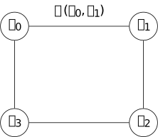
The four-cycle illustrates the kernel product. Every edge contributes the same function \(K\) of its endpoints. Each site's two mass contributions add to \(m^2x_j^2/2\); closing the last edge identifies \(x_4\) with \(x_0\).
Theorem 2. Hermite diagonalization [fdip-007U]AGENTDRAFTED
- November 1, 2026
Theorem 2. Hermite diagonalization [fdip-007U]AGENTDRAFTED
- November 1, 2026
For the Gaussian transfer operator, define \[\begin {aligned} \cosh \omega &=1+\frac {m^2}{2w},& \omega &>0,\\ q&=e^{-\omega },& s&=w\sinh \omega ,\\ \lambda _0&=\sqrt {\frac {2\pi }{w}}e^{-\omega /2}. \end {aligned}\] Define the probabilists' Hermite polynomials \(\operatorname {He}_n\) by the generating function \[e^{uz-z^2/2} =\sum _{n=0}^\infty \operatorname {He}_n(u)\frac {z^n}{n!},\] and put \[h_n^s(x)=\left (\frac {s}{\pi }\right )^{1/4} \frac {\operatorname {He}_n(\sqrt {2s}\,x)}{\sqrt {n!}} e^{-sx^2/2}.\] These functions form an orthonormal basis of \(L^2(\mathbb R,dx;\mathbb C)\), and \[Th_n^s=\lambda _0q^nh_n^s\qquad (n\ge 0).\] Consequently \(T\) is positive, injective and trace class, with \(\|T\|=\lambda _0\) and \(\operatorname {Tr}T=\lambda _0/(1-q)\). The normalized operator \(\widehat T=T/\lambda _0\) is an injective positive contraction.
Proof.
- November 1, 2026
Proof.
- November 1, 2026
First establish the basis. Integrating two generating functions against \(e^{-sx^2}\) gives \[\begin {aligned} &\int _{\mathbb R}e^{-sx^2} e^{\sqrt {2s}\,xz-z^2/2} e^{\sqrt {2s}\,xt-t^2/2}\,dx\\ &\hspace {20mm}=\sqrt {\frac \pi s}\,e^{zt}. \end {aligned}\] Differentiation at \(z=t=0\) proves orthogonality with precisely the displayed normalization. Every such differentiation is justified by a polynomial times an integrable Gaussian, uniformly for the complex parameters in a compact set.
For completeness, suppose \(f\in L^2\) is orthogonal to every \(h_n^s\). Since \(\operatorname {He}_n\) has degree \(n\) and leading coefficient one, all moments of \(g(x)=f(x)e^{-sx^2/2}\) vanish. Cauchy–Schwarz shows that \(g\in L^1\) and that \[F(z)=\int _{\mathbb R}g(x)e^{zx}\,dx\] is entire: on every compact set of complex \(z\), all derivative integrands have an integrable majorant of the form \(|f(x)|\,|x|^k e^{-sx^2/2+R|x|}\). All Taylor coefficients of \(F\) vanish, so \(F=0\); in particular the Fourier transform of \(g\) vanishes. To see the needed uniqueness directly, convolve \(g\) with a normalized Gaussian. The Gaussian Fourier integral and Fubini express this convolution as an integral of its zero Fourier transform, hence it is zero. As the Gaussian variance tends to zero, these convolutions tend to \(g\) in \(L^1\), by continuity of translations in \(L^1\) and dominated convergence. Thus \(g=0\) almost everywhere and \(f=0\). The orthonormal family is complete.
Now diagonalize the kernel. With \(a=w\cosh \omega /2\), the identities \(s=w\sinh \omega \) and \(a+s/2=w/(2q)\) give, by completing the square in \(y\), \[\begin {aligned} &\int _{\mathbb R}K(x,y)e^{-sy^2/2} e^{\sqrt {2s}\,yz-z^2/2}\,dy\\ &\hspace {8mm}=\lambda _0e^{-sx^2/2} e^{\sqrt {2s}\,xqz-q^2z^2/2}. \end {aligned}\] The constant is \(\sqrt {\pi /(a+s/2)}=\sqrt {2\pi q/w}=\lambda _0\). Differentiating \(n\) times at zero, again under a Gaussian majorant, gives \(Th_n^s=\lambda _0q^nh_n^s\).
If \(f=\sum _n c_nh_n^s\), boundedness and completeness give \[Tf=\sum _{n=0}^\infty \lambda _0q^nc_nh_n^s\] in \(L^2\). Every eigenvalue is strictly positive, which proves positivity and injectivity. Their maximum is \(\lambda _0\). For a positive compact operator, being trace class means that these eigenvalues have finite sum; here the sum is \(\lambda _0/(1-q)\). This proves all operator assertions. It also gives the Mehler kernel expansion \[K(x,y)=\sum _{n=0}^\infty \lambda _0q^nh_n^s(x)h_n^s(y)\] in \(L^2(\mathbb R^2)\): the squared Hilbert–Schmidt norm of the tail is \(\lambda _0^2\sum _{n>r}q^{2n}\) after truncation at \(r\). This convergence statement suffices for the operator identity.
The calculation is a direct diagonalization of
Definition 1. TauCeti's
TauCeti.hermiteHilbertBasis and
TauCeti.coe_hermiteHilbertBasis
supply the complete orthonormal Hermite basis at \(s=1\), with
exactly the probabilists' normalization used here. The unitary
dilation \(f(x)\mapsto s^{1/4}f(\sqrt {s}\,x)\) gives the displayed
basis for general \(s>0\). These references support the basis;
the kernel eigenvalues and transfer properties are proved above.
Example 3. A transfer norm greater than one [fdip-007X]AGENTDRAFTED
- November 1, 2026
Example 3. A transfer norm greater than one [fdip-007X]AGENTDRAFTED
- November 1, 2026
Take \(w=3/2\) and \(m^2=4/5\) in Theorem 2. Then \[\begin {aligned} \cosh \omega &=\frac {19}{15},& s&=\frac {\sqrt {34}}5,\\ q&=\frac {19-2\sqrt {34}}{15},& \lambda _0&=\sqrt {\frac {4\pi q}{3}}. \end {aligned}\] Numerically \(\omega \approx 0.714971\) and \(\lambda _0\approx 1.431497\). In particular \(\|T\|=\lambda _0>1\). This inequality does not depend on rounding: \(\sqrt {34}<6\) gives \(q>7/15\), and \(\pi >3\) gives \(\lambda _0^2>28/15>1\).
All eigenvalues are nevertheless positive: \(\lambda _n=\lambda _0q^n\). Dividing by the leading eigenvalue gives \(\widehat T h_n^s=q^nh_n^s\) and \(\|\widehat T\|=1\). The lowest mode label \(n=0\) refers to the Gaussian function \(h_0^s\), not to a constant function on \(\mathbb R\); the latter does not belong to Lebesgue \(L^2\). Thus the normalization is a genuine scalar factor in the operator, fixed by the chosen reference measure.
Theorem 4. Periodic traces and field correlations [fdip-007V]AGENTDRAFTED
- November 1, 2026
Theorem 4. Periodic traces and field correlations [fdip-007V]AGENTDRAFTED
- November 1, 2026
Use the kernel and parameters of Definition 1 and Theorem 2. For every integer \(N\ge 1\), \[\operatorname {Tr}T^N =\frac {\lambda _0^N}{1-q^N} =\frac {(2\pi /w)^{N/2}}{2\sinh (N\omega /2)}.\] For \(N\ge 3\), this equals the periodic Gaussian normalizer \(Z_N\). If \(f_0,\ldots ,f_{N-1}\) are bounded complex measurable functions and \(M_f\) denotes multiplication by \(f\), then \[\mathbb E_{\mu _N}\prod _{j=0}^{N-1}f_j(x_j) =\frac {\operatorname {Tr} (M_{f_0}T M_{f_1}T\cdots M_{f_{N-1}}T)}{Z_N}.\] In particular, bounded two-point observables have the usual cyclic trace expression with \(T^{N-t}\) and \(T^t\).
For \(N\ge 3\) and the unbounded coordinate observable, let \(Xf(x)=xf(x)\) on its domain \(\{f\in L^2:xf\in L^2\}\). For integers \(0\le t\le N\), initially on finite Hermite sums, put \[A_t=T^{t/2}XT^{(N-t)/2}.\] It has a unique Hilbert–Schmidt extension. The precise coordinate trace formula is \[\begin {aligned} \mathbb E_{\mu _N}[x_0x_t] &=\frac {\operatorname {Tr}(A_t^*A_t)}{Z_N}\\ &=\frac {q^t+q^{N-t}}{2s(1-q^N)}, \qquad x_N=x_0. \end {aligned}\] Here \(\operatorname {Tr}(A_t^*A_t)\) supplies the meaning of the frequently written unbounded expression \(\operatorname {Tr}(T^{N-t}XT^tX)\).
Proof.
- November 1, 2026
Proof.
- November 1, 2026
The eigenvalues in Theorem 2 give the first trace by a geometric sum. The remaining expression uses \(\lambda _0=\sqrt {2\pi /w}\,q^{1/2}\) and \(q^{-N/2}-q^{N/2}=2\sinh (N\omega /2)\). On the ordinary cycle, the precision is \(Q_N=m^2I+wL_{C_N}\). The twisted-cycle determinant at trivial holonomy, with the scalar factor \(w\) restored, gives \[\det Q_N=w^N\bigl (2\cosh (N\omega )-2\bigr ).\] The real Gaussian integral therefore gives exactly the same \(Z_N\). The trace identity for \(N=1,2\) remains an operator identity; no ordinary simple-cycle identification is used for those two periods.
For bounded insertions, \(M_fT\) is Hilbert–Schmidt. The product of two such operators is trace class; multiplying by the remaining bounded factors preserves this property. The Hilbert–Schmidt kernel trace identity \[\operatorname {Tr}(AB)=\int _{\mathbb R^2}A(x,y)B(y,x)\,dx\,dy\] follows by expanding the two kernels in an orthonormal basis and taking their \(L^2\) pairing. Applying it to the cyclic product and composing the intervening kernels yields \[\operatorname {Tr}(M_{f_0}T\cdots M_{f_{N-1}}T) =\int _{\mathbb R^N}\prod _j f_j(x_j) \prod _jK(x_j,x_{j+1})\,d^Nx.\] All repeated integrals are absolutely convergent: the absolute integrand is bounded by \(\prod _j\|f_j\|_\infty \) times the integrable massive Gaussian. The kernel factorization in Definition 1 proves the asserted expectation.
For the coordinate insertion, the Hermite generating function gives the recurrence \[Xh_n^s=\frac {\sqrt {n+1}\,h_{n+1}^s +\sqrt n\,h_{n-1}^s}{\sqrt {2s}},\] where the second term is zero at \(n=0\). Consequently the matrix of \(A_t\) has only two adjacent diagonals. Summing their squared entries gives \[\begin {aligned} \|A_t\|_{\mathrm {HS}}^2 &=\frac {\lambda _0^N}{2s} \frac {q^t+q^{N-t}}{(1-q^N)^2}. \end {aligned}\] The sum is finite also at \(t=0,N\). Thus the operator on the dense finite Hermite span extends uniquely to a Hilbert–Schmidt operator. Thus \(A_t^*A_t\) is positive trace class and its trace is this squared norm. Division by \(Z_N\) gives the displayed value. Finally, the periodic covariance calculation, with \(s=w\sinh \omega \), gives this same value for \((Q_N^{-1})_{0t}\). Gaussian covariance therefore identifies it with \(\mathbb E_{\mu _N}[x_0x_t]\), including the periodic endpoint. No cyclic manipulation of an undefined unbounded product is used.
This finite periodic calculation makes the trace notation of [wingate2025lattice, Eq. (5.4), p. 4] explicit for the Gaussian chain. That source subsequently takes an infinite-time limit; the identities here hold at finite \(N\). The Ising transfer and Markov-chain comparison in [friedli2017statistical, Section 3.10.4, p. 139] concerns a different state space and is background for the transfer interpretation, not a premise for this Gaussian proof.
Corollary 5. The oscillator Hamiltonian [fdip-007W]AGENTDRAFTED
- November 1, 2026
Corollary 5. The oscillator Hamiltonian [fdip-007W]AGENTDRAFTED
- November 1, 2026
For the normalized transfer operator \(\widehat T=T/\lambda _0\) of Theorem 2, the transfer Hamiltonian is the spectral logarithm \(H=-\log \widehat T\). Explicitly, if \(f=\sum _{n\ge 0}c_nh_n^s\), its domain and action are \[\begin {aligned} D(H)&=\left \{f:\sum _{n=0}^\infty (n\omega )^2|c_n|^2<\infty \right \},\\ Hf&=\sum _{n=0}^\infty n\omega c_nh_n^s. \end {aligned}\] It is nonnegative and self-adjoint, with eigenvalues \(n\omega \). Its zero eigenspace is the line spanned by \(h_0^s\), and its mass gap is \(\omega \). It is unbounded even though \(\widehat T\) is bounded and injective.
On the finite Hermite span, it has the differential expression \[Hf=\frac \omega {2s} \left (-f''+s^2x^2f-sf\right ).\] The closure of this expression on that span is the above spectral operator. This is the harmonic oscillator with its ground energy subtracted. The time step has length one; a specified step \(a_t>0\) instead gives \(H/a_t\) and gap \(\omega /a_t\).
Proof.
- November 1, 2026
Proof.
- November 1, 2026
The unitary coefficient map \(f\mapsto (c_n)\) identifies \(\widehat T\) with multiplication by \(q^n>0\) on \(\ell ^2\). Its negative logarithm is multiplication by \(n\omega \) on the stated maximal domain. A real diagonal operator on that domain is self-adjoint; its quadratic form is nonnegative. The listed eigenspaces, spectrum and gap follow directly, and \(\|Hh_n^s\|=n\omega \) proves unboundedness. Finite coefficient truncations converge both in norm and after applying \(H\), so the finite Hermite span is a core.
Differentiating the Hermite generating function and comparing coefficients gives \(\operatorname {He}_n''(u)-u\operatorname {He}_n'(u) +n\operatorname {He}_n(u)=0\). Substitution into the definition of \(h_n^s\) yields \[-(h_n^s)''+s^2x^2h_n^s=(2n+1)s\,h_n^s.\] The displayed differential expression therefore acts as \(n\omega \) on every basis vector. The core statement proves that its closure is exactly \(H\).
TauCeti's
TauCeti.hermiteFunction_oscillator
proves the pointwise differential identity at \(s=1\) for the
same normalized Hermite functions. Dilation gives the identity
above for \(s>0\); the spectral logarithm, its domain and the
closure statement are supplied by the preceding argument.
The logarithmic prescription follows [wingate2025lattice, Eq. (5.5), p. 4], with the leading transfer eigenvalue removed explicitly. It constructs the Hamiltonian for a Gaussian model of finite spatial volume. No limit in time, spatial volume or lattice spacing is needed.