Notes on formulating discrete-induced physics [fdip-0001]
- November 3, 2026
- Utensil Song
Notes on formulating discrete-induced physics [fdip-0001]
- November 3, 2026
- Utensil Song
Physics often models length, time and field values as continuous (infinitely divisible) quantities. Measurements have finite resolution, so they do not establish that this continuum is fundamental. The real numbers are its usual mathematical form. The hypothesis is that geometry, time and matter can be induced from finite carriers and exact algebra, with continuum physics recovered at large scales. A classical field assigns values to points of space; in this discrete setting, the points are vertices or edges of a finite graph. Finitely many coordinates need not mean finitely many possible values: later Gaussian probability laws are laws on a real inner-product space. What a structure induces is kept separate from what must be supplied. A finite incidence presentation records the finite vertex set, edge set and endpoint maps; the alternating four-cycle of Example 1.8 makes the additional weights explicit. Reordering vertices changes a representation; changing weights changes the model. Gaussian elimination in Elimination and retained observables uses a specified quadratic action and reference measure.
Induced geometry provides one motivation. On a fixed background, one-loop matter fluctuations generate an Einstein-Hilbert term in the effective action [visser2002sakharov, Section 1, Eq. (1)], so the gravitational action need not be assumed: it can be induced by the matter content. Keeping supplied microscopic data, state assumptions and induced structure apart is then a distinction with content. Conjecture 42.1.1 asks for an arithmetic scheme with a Clifford sheaf and a finite-group action, for a map from a moduli stack controlling the continuum limit and the background dependence, and for quantum-field-theory parameters given by special L-values. Spacetime, physical parameters, the Standard Model equations and gravitational equations stay outside those finite constructions. Discrete induction and its open interfaces records the comparisons that remain open: the physical environment map, and the continuum question, which is asked and not answered. The groupoid and the realization do not supply a site, a stack, or a descent. No moduli map is constructed.
These notes develop finite constructions and do not propose a physical theory. The parts run from fields on finite carriers through Gaussian laws, symmetry and Clifford algebras, to arithmetic families and a fixed-mode comparison on a supplied circle. Geometric realization then asks which information survives when weights are forgotten. Selected backgrounds, gauge fields, Euclidean time and lattice fermions give the finite constructions that the structure chapters and the closing § 42 compare. Remark [fdip-004E] maps the parts. The alternating four-cycle returns as the example that ties a later construction to specified fields, weights and observables.
Remark. How to read these notes [fdip-004E]AGENTDRAFTED
- November 3, 2026
Remark. How to read these notes [fdip-004E]AGENTDRAFTED
- November 3, 2026
The reading route has 14 parts. The diagrams show selected prerequisites for reading, not every premise of every result. An arrow means that its destination uses a construction or comparison from its source. Each statement still gives its precise hypotheses. Questions on the arrows motivate the next topic; they do not assert that the notes already derive the corresponding physics.
The overview includes the full intended route. The prime-by-prime Gaussian extension, Structure and the concluding comparison of fixed and free data are published. The Grassmann integration chapter, fermionic elimination, covariant Dirac operators and the Wilson term develop the fermion part. The compatibility test fixes one finite spinor datum. The larger proposals remain open tests. A solid arrow into open material records an intended prerequisite, not a result already proved. In the part diagrams, a dotted box names a neighboring part; every arrow is solid.
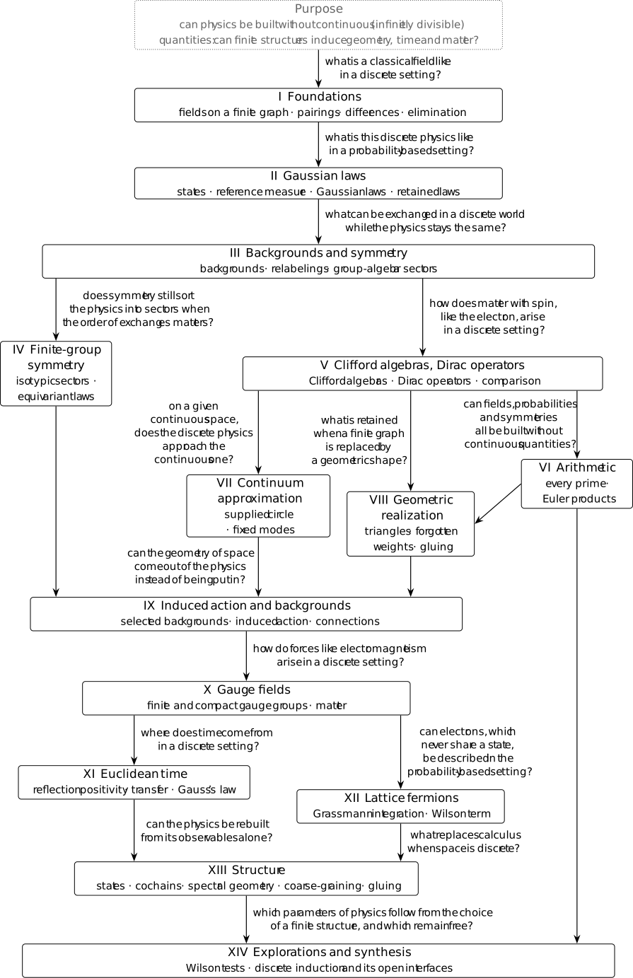
After backgrounds and symmetry, the route separates finite-group sectors from Clifford algebras and spatial Dirac operators. The latter lead to arithmetic, approximation on a supplied circle and geometric realization. These are not three independent branches: the fiber-constancy criterion remains in Arithmetic and is used by Realization. The direct comparison from Part V also remains visible. The figures therefore show selected prerequisites, not an exact transitive reduction of all dependencies.
Finite-group sectors, circle approximation and realization meet in the study of selected backgrounds and induced actions. Connections lead to gauge fields; Euclidean time and the fermion branch then feed the Structure part. The fermion branch currently supplies its Grassmann integration, elimination, covariant Dirac operators and the free Wilson remedy. The arrow from gauge fields to Euclidean time meets the gauge transfer and Gauss's law. Reflection positivity alone does not supply that shift. The arrow from gauge fields to lattice fermions meets the covariant Dirac operator and the free Wilson remedy above, not Grassmann integration or fermionic elimination, and it does not identify those operators with a physical electron. Arithmetic and Structure contribute different questions to the closing explorations. These destinations are earned by specific finite constructions, rather than adopted as starting axioms.
- Part I, Foundations: fields on finite carriers, reference pairings, differences and algebraic elimination.
- Part II, Gaussian laws: states, reference measure, positive and constrained Gaussian laws, and retained observables.
- Part III, Backgrounds and symmetry: transported data, observables and half-turn sectors.
- Part IV, Finite-group symmetry: real isotypic projectors, multiplicities and Gaussian sector laws.
- Part V, Clifford algebras, spatial Dirac operators and enriched comparison: distinct questions about quadratic forms, first-order operators and preserved observables.
- Part VI, Arithmetic families, followed by the Gaussian extension at every prime.
- Part VII, Continuum approximation: a supplied circle and fixed Fourier modes, not a general emergent continuum.
- Part VIII, Geometric realization: which information survives a replacement by a shape, including the weights it can forget.
- Part IX, Selected backgrounds, induced actions and interactions, local laws and gluing, and connections and holonomy.
- Part X, Gauge fields: finite surface laws, matter-induced actions, dynamical connections and compact groups.
- Part XI, Euclidean time: reflected pairings, explicit transfer operators and Gauss's law. Reflection positivity alone does not supply a time shift.
- Part XII, Lattice fermions: finite Grassmann integration, determinants, Pfaffians, Wick identities and elimination, followed by covariant Dirac operators and doubling and the Wilson remedy.
- Part XIII, Structure: operator-algebra, cochain, spectral-geometry, coarse-graining and gluing questions, developed in the chapters of that part. Speculative and optional sections retain those qualifications.
- Part XIV, Explorations and synthesis: the existing conjecture and finite interfaces, the compatibility test, and a comparison of what is fixed or free. The larger proposals remain open tests. The synthesis records the remaining open comparisons: the physical environment map, the continuum question, asked and not answered, with no moduli map claimed, and geometric or moduli structure beyond the published groupoid and realization.
The part diagrams appear at their openings. The Structure diagram routes its time input to the transfer chapter and its fermion input to the Dirac-Kähler chapter, where those suppliers are actually intended. It does not make the earlier states or cochains definitions consequences of time evolution or fermions. The root retains one linear reading order; forward examples and open questions orient that reading without becoming premises of the preceding proofs.
1. Finite fields and operator products [fdip-0015]AGENTDRAFTED
- October 20, 2026
1. Finite fields and operator products [fdip-0015]AGENTDRAFTED
- October 20, 2026
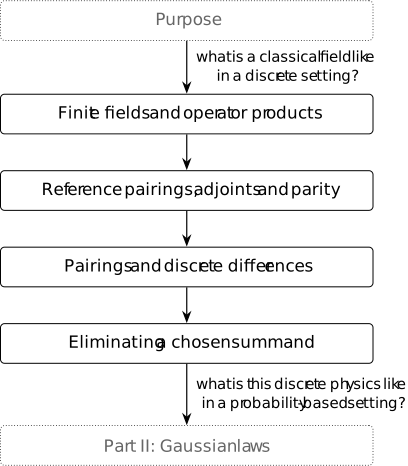
The coefficient ring is commutative and unital; the operator product need not commute. Positive counting pairings and weights enter in the real specialization. Working over a ring first separates identities of incidence, composition and elimination from positivity and integration. The general adjoint construction assumes perfect pairings, and elimination requires an invertible eliminated block; these hypotheses do not follow from the coefficient ring alone. Real positivity and measure are additional data for the later Gaussian laws.
A measurement has finite resolution, and a lattice regularisation keeps finitely many sites. Both give finite data, while the field equations are written for a continuum. Can the continuum be induced from finite data? An answer must begin with a field on finitely many points: a value at each point, or along each step between them.
Discussion 1.1. The field equations in three languages [fdip-00AA]AGENTDRAFTED
- November 4, 2026
Discussion 1.1. The field equations in three languages [fdip-00AA]AGENTDRAFTED
- November 4, 2026
In the undergraduate course on electromagnetism the field equations arrive in the language of vector calculus. With a charge density \(\rho \) and a current \(J\), and with the constants set to one, they read \[\operatorname {div} E=\rho ,\qquad \operatorname {div} B=0,\qquad \operatorname {curl} E=-\partial _t B,\qquad \operatorname {curl} B=\partial _t E+J.\] 4 equations, two vector fields, and a potential \(A\) that enters when one wants to solve them. There the potential is primitive and the fields are derived from it by a gradient, and the metric sits in the operators: the divergence, the curl and the cross product all know about lengths and angles. Every object is continuous as well: \(\rho \) is a density, and \(\partial _t\) presupposes a parameter along which to differentiate.
A course in mathematical physics rewrites the system in the language of differential forms. The potential becomes a \(1\)-form \(A\) and the field strength its exterior derivative \(F=dA\). The exterior derivative needs no metric, so \(dF=0\) is a consequence of \(d\circ d=0\) rather than an equation to impose, and gauge transformations \(A\mapsto A+d\chi \) leave \(F\) unchanged by construction, which is why gauge theory is written this way. The metric reappears in the Hodge star that the equations with sources require, \(d\star F=\star j\), while \(d\) raises the degree of a form. [hassani2013mathematical, Section 28.5] writes the field equations this way.
Readers who have met geometric calculus will recognize the same system in the unified language that Hestenes and Sobczyk proposed for mathematics and physics. The electric and magnetic fields are then grades of one object, the bivector \(F=E+IB\), where \(I\) is the pseudoscalar of the algebra, the product of the 4 frame vectors, with \(I^2=-1\), so the magnetic field enters as the dual bivector \(IB\), and the pair forms one bivector rather than the vector and pseudovector of vector calculus. The derivative is the vector derivative \(\nabla \): the derivative along each direction of a chosen frame, combined into a single vector-valued operator by the geometric product with the frame vectors. It acts by geometric multiplication, and a vector multiplied that way by a multivector splits into two parts, \[\nabla F=\nabla \cdot F+\nabla \wedge F,\] an inner product giving a divergence and an outer product giving a curl. With it the 4 equations become \(\nabla F=J\), the divergence part carrying the sources and the curl part vanishing, so each original equation returns as a definite grade. Hestenes and Sobczyk develop the calculus [hestenes2012clifford], Doran and Lasenby carry it through classical electrodynamics [doran2003geometric, Section 7.1], and Macdonald's textbook is the treatment [macdonald2012vector]. Here one algebra and one derivative serve both objects, and the metric is neither an operator nor a dual: it is inside the geometric product, which is why the language carries a chosen spacetime with it.
All three ways of writing these equations need a limit: in each, a derivative compares values at points whose separation shrinks. Those points are not bare: the continuum carries a metric, a topology and a smooth structure, and that is what gives a separation, a direction and a gradient their meaning. On a lattice only finitely many points remain, and a direction becomes a step from one site to a neighbour. What is left of the gradient is the difference of the values at the two ends of each step. A derivative of a product obeys the Leibniz rule; does a difference of values obey it as well, or does something else take its place? And which changes of the potential does a difference fail to see?
A field assigns a coefficient to each vertex or edge. Along an oriented edge, the incidence map subtracts the source value from the head value. Endpoint pullbacks express this comparison between distinct field spaces. Composition supplies an operator product on a common field module; comparing it with pointwise field multiplication gives a discrete product rule. Lemma 1.20 states that rule, and Example 1.22 shows where operator commutativity fails. The alternating four-cycle of Example 1.8 supplies the weights and the half-turn that the examples below use.
Definition 1.2. Ring-valued incidence fields [fdip-0010]AGENTDRAFTED
- October 20, 2026
Definition 1.2. Ring-valued incidence fields [fdip-0010]AGENTDRAFTED
- October 20, 2026
Let \(R\) be a commutative ring with identity. Choose finite sets \(V,E\) and maps \(s,h:E\to V\). The edge \(e\) goes from \(s(e)\) to \(h(e)\); loops and distinct edges with the same endpoints are allowed. Call the finite sets together with their endpoint maps the carrier. The field modules are the vertex-field module and the edge-field module \[\mathcal F_R(V)=\{f:V\to R\},\qquad \mathcal F_R(E)=\{a:E\to R\}.\] Addition, scalar multiplication and multiplication are pointwise: \[(f+g)(v)=f(v)+g(v),\quad (rf)(v)=rf(v),\quad (fg)(v)=f(v)g(v).\] These are modules and commutative unital \(R\)-algebras; the unit is the constant field \(1\).
The zero ring and an empty vertex set or edge set are allowed. On an empty set there is one field, and the constant \(1\) is also zero. No nontriviality, pairing, retained subset or positivity is assumed. The algebra convention is [stacks2017stacks, Section 22.2], Tag 09JF. The module and algebra laws are in Lemma 1.5.
The alternating four-cycle of Example 1.8 is an instance of these fields.
Definition 1.3. Pullbacks and the incidence map [fdip-00AQ]AGENTDRAFTED
- November 4, 2026
Definition 1.3. Pullbacks and the incidence map [fdip-00AQ]AGENTDRAFTED
- November 4, 2026
Let \(R\) be a commutative ring with identity, with the carrier of finite sets \(V,E\) and maps \(s,h:E\to V\), and the field modules over it. For a map \(a:E\to V\), its field pullback is \[a^*:\mathcal F_R(V)\to \mathcal F_R(E),\qquad (a^*f)(e)=f(a(e)).\] It preserves addition, scalars, products and the unit. The ring-valued incidence map is the typed difference \[d=h^*-s^*:\mathcal F_R(V)\longrightarrow \mathcal F_R(E).\] Thus \((df)(e)=f(h(e))-f(s(e))\). This is an \(R\)-linear map, with both coefficient rings equal to \(R\) and scalar homomorphism \(\sigma =\operatorname {id}_R\), as in Remark [ca-001G]. The two field modules need not coincide, so \(d^2\) has no meaning without an additional composable map. The pullback law, the linearity and the kernel of \(d\) are in Lemma 1.5.
For real oriented-graph incidence, see [spielman2009effective, Section 2.1, p. 4]; the ring-level claims follow from Lemma 1.5.
Remark 1.4. Incidence and the exterior derivative [fdip-00AB]AGENTDRAFTED
- November 4, 2026
Remark 1.4. Incidence and the exterior derivative [fdip-00AB]AGENTDRAFTED
- November 4, 2026
The potential of the preceding discussion is a field on the vertices: one value per site, added and scaled pointwise as in the vertex-field module. Along an edge the difference between the two endpoint values is what the edge carries, so the ring-valued incidence map takes a potential to the field strength read off the edges. On a cubic lattice whose steps are \(x\to x+\mu \), that difference is \(\varphi (x+\mu )-\varphi (x)\).
In the forms notation the potential is a \(0\)-form and the field strength a \(1\)-form, related by \(d\). The incidence map plays the role of \(d\) on \(0\)-forms, and it is not \(d\): the exterior derivative raises the degree of a form, while the incidence map runs from vertex fields to edge fields of one particular graph. A field pullback is composition with a map of the two finite sets, as in the substitution \(f'(x)=f(h(x))\).
Lemma 1.5. Basic properties of incidence fields [fdip-00AC]AGENTDRAFTED
- November 3, 2026
Lemma 1.5. Basic properties of incidence fields [fdip-00AC]AGENTDRAFTED
- November 3, 2026
Let \(R\) be a commutative unital ring, and let \(V,E,s,h\) and the field modules, field pullback and ring-valued incidence map be as in the two definitions above. The pointwise operations make both modules commutative unital \(R\)-algebras, the indicator fields are a basis of each, every field pullback preserves the operations, and \(d\) is \(R\)-linear. Call two vertices equivalent when they are equal or a finite sequence of edges has them as successive ends, ignoring orientation. The equivalence classes are the undirected components; a vertex that lies on no edge is a component of its own. Then \(df=0\) if and only if \(f\) is constant on each undirected component.
Proof.
- November 3, 2026
Proof.
- November 3, 2026
Every module and algebra identity follows by evaluation from the corresponding identity in \(R\). For each \(v\in V\), let \(\delta _v(u)\) be \(1\) if \(u=v\) and \(0\) otherwise. Evaluation at \(u\) proves \[f=\sum _{v\in V}f(v)\delta _v,\] and proves uniqueness of the coefficients. The same argument applies to edge fields. On an empty carrier the sum is empty and there is one field. Evaluation also proves every pullback law; for instance \(a^*(fg)(e)=f(a(e))g(a(e))\). Finally \[d(rf+g)(e)=r\bigl (f(h(e))-f(s(e))\bigr )+g(h(e))-g(s(e)),\] which proves linearity. These evaluations apply to the zero ring.
If \(df=0\), then \(f(h(e))=f(s(e))\) for every edge, so \(f\) takes the same value at the successive ends of any finite sequence of edges and is constant on each component. Conversely, the two ends of an edge lie in one component, and the two ends of a loop are the same vertex, so a field constant on each component has \(df=0\). The argument uses no division.
Remark 1.6. Gauge freedom of a potential [fdip-00AD]AGENTDRAFTED
- November 3, 2026
Remark 1.6. Gauge freedom of a potential [fdip-00AD]AGENTDRAFTED
- November 3, 2026
The kernel in Lemma 1.5 is the gauge freedom of the potential. Adding a constant on one undirected component leaves every edge difference unchanged, and the electric field is the negative of that difference. A vector potential is assigned to the edges, as the link variables of lattice gauge theory are, and its field strength is the difference of those values around a face. The identity \(d\circ d=0\) needs that second difference, from edge fields to face fields. The maps defined here run only from vertices to edges.
Definition 1.7. The incidence matrix [fdip-00AF]AGENTDRAFTED
- November 3, 2026
Definition 1.7. The incidence matrix [fdip-00AF]AGENTDRAFTED
- November 3, 2026
Let \(R\) be a commutative unital ring, and let \(d\) be the ring-valued incidence map of a finite carrier \(\,(V,E,s,h)\). Choose orders of the vertex and edge indicators. Let \(c_V:\mathcal F_R(V)\to R^{|V|}\) and \(c_E:\mathcal F_R(E)\to R^{|E|}\) send a field to its ordered values. The indicator expansion in Lemma 1.5 gives their inverses, where \(\delta _v\) is the indicator field of a vertex \(v\). The incidence matrix represents \(c_Edc_V^{-1}\): \[B_{ev}=(d\delta _v)(e)=\mathbf 1_{v=h(e)}-\mathbf 1_{v=s(e)}.\] Rows are indexed by edges and columns by vertices. A loop has a zero row; reversing an edge negates its row. This extends the oriented-graph sign convention of [spielman2009effective, Section 2.1, p. 4]. If coordinate reorderings are \(P_V,P_E\), then \(B'=P_EBP_V^{-1}\), since both sides send \(c'_V(f)\) to \(c'_E(df)\).
Example 1.8. The alternating four-cycle [fdip-0003]AGENTDRAFTED
- October 16, 2026
Example 1.8. The alternating four-cycle [fdip-0003]AGENTDRAFTED
- October 16, 2026
Let \(V=\mathbb Z/4\mathbb Z\) and \(E=\{e_0,e_1,e_2,e_3\}\), with \(s(e_i)=i\) and \(h(e_i)=i+1\) modulo \(4\). For \(t>0\), assign weights \[w_t(e_0)=w_t(e_2)=1,\qquad w_t(e_1)=w_t(e_3)=t.\] This is a weighted finite incidence presentation: the parameter \(t\) is supplied, and every edge weight is positive.
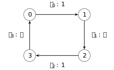
Each arrow points from source to head; the label gives its edge name and weight. A half-turn exchanges opposite vertices and edges.
On the real four-cycle, order vertices as \(0,1,2,3\) and edges as \(e_0,e_1,e_2,e_3\). The incidence matrix \(B\) of \(D\), and the coordinate array \(W_t\) of the weights, are \[B=\begin {pmatrix} -1&1&0&0\\ 0&-1&1&0\\ 0&0&-1&1\\ 1&0&0&-1 \end {pmatrix},\qquad W_t=\operatorname {diag}(1,t,1,t).\] Thus a field with ordered values \((a,b,c,d)\) has edge differences \((b-a,c-b,d-c,a-d)\). For \(f=\delta _1\), the edge values of \(Df\) are \((1,-1,0,0)\): the field rises along \(e_0\) and falls along \(e_1\).
The quadratic action of Example 7.4 uses these same edge orientations and weights, with a positive mass term.
Define the half-turn on both sets by \[r_V(i)=i+2,\qquad r_E(e_i)=e_{i+2}.\] Applying either map twice adds 4, so both are involutions, and \(r_V(0)=2\) shows that the map on vertices is not the identity. Moreover, \[s(r_E(e_i))=i+2=r_V(s(e_i)),\] \[h(r_E(e_i))=i+3=r_V(h(e_i)).\] The half-turn therefore preserves the directed incidence data. Since \(i\) and \(i+2\) have the same parity, it also preserves the weights: \(w_t(r_E(e_i))=w_t(e_i)\). In contrast, a one-step rotation sends \(e_0\) to \(e_1\) and fails to preserve weights when \(t\ne 1\).
After forgetting orientations and weights, the underlying graph is
Mathlib's SimpleGraph.cycleGraph at 4 vertices, identifying
\(\operatorname {Fin}(4)\) with the residue classes modulo \(4\). That
declaration specifies the unweighted graph. The displayed matrix and
weight-preserving half-turn follow from the substitutions above.
Remark 1.9. Divergence and the discrete Poisson equation [fdip-00AG]AGENTDRAFTED
- November 3, 2026
Remark 1.9. Divergence and the discrete Poisson equation [fdip-00AG]AGENTDRAFTED
- November 3, 2026
The incidence matrix \(B\) is the difference matrix of the preceding discussion, and \(L=B^{\mathsf T}B\) is the graph Laplacian. The matrix \(-B^{\mathsf T}\) is the discrete divergence. With the edge field \(E=-B\varphi \), Gauss's law \(\nabla \cdot E=\rho \) becomes \[\,(-B^{\mathsf T})(-B\varphi )=B^{\mathsf T}B\varphi =L\varphi =\rho ,\] the discrete Poisson equation. Computations, and the later Laplacian chapters, use \(d\) in this matrix form.
Discussion 1.10. Products and derivatives [fdip-00AH]AGENTDRAFTED
- November 4, 2026
Discussion 1.10. Products and derivatives [fdip-00AH]AGENTDRAFTED
- November 4, 2026
A coupling that varies from site to site enters a lattice action as a coefficient: the term \(m\sum _v\varphi (v)^2\) for a constant mass \(m\) becomes \(\sum _v m(v)\varphi (v)^2\), so a fixed field multiplies the field at each site. Multiplying by a fixed field and taking differences along the edges are then two linear maps of one module, and composing them in the two orders gives two different maps. What is the map that multiplies, and how badly does it fail to commute with a difference?
Definition 1.11. Multiplication operators [fdip-00AI]AGENTDRAFTED
- November 3, 2026
Definition 1.11. Multiplication operators [fdip-00AI]AGENTDRAFTED
- November 3, 2026
Let \(R\) be a commutative unital ring and \(V\) a finite set. On the vertex-field module, each \(f\in \mathcal F_R(V)\) determines a multiplication operator \[M_f:\mathcal F_R(V)\to \mathcal F_R(V),\qquad M_f(g)=fg.\] The assignment \(f\mapsto M_f\) is an injective \(R\)-algebra map, \[M_{f+g}=M_f+M_g,\quad M_{rf}=rM_f,\quad M_{fg}=M_fM_g,\quad M_1=I.\] Proposition 1.13 proves these identities from the ring laws.
Remark 1.12. The potential term [fdip-00AJ]AGENTDRAFTED
- November 3, 2026
Remark 1.12. The potential term [fdip-00AJ]AGENTDRAFTED
- November 3, 2026
The multiplication operator \(M_V\) is the potential term of a lattice Schrödinger operator, added to a difference operator. The assignment \(f\mapsto M_f\) is how a field acts on its own module, and \(M_f M_g=M_g M_f\). A shift need not commute with \(M_f\). That product is the operator product of Proposition 1.13, and Example 1.22 computes the failure on a cycle.
Proposition 1.13. Composition and field multiplication [fdip-0011]AGENTDRAFTED
- October 20, 2026
Proposition 1.13. Composition and field multiplication [fdip-0011]AGENTDRAFTED
- October 20, 2026
Let \(R\) be a commutative unital ring. For \(R\)-modules \(M,N,P\), use \(\operatorname {Hom}_R(M,N)\) for additive, scalar-preserving maps. Thus linearity fixes \(\sigma =\operatorname {id}_R\). Given \(A\in \operatorname {Hom}_R(M,N)\) and \(B\in \operatorname {Hom}_R(N,P)\), write \[BA=B\circ A:M\to P.\] Composition is associative and \(R\)-bilinear where the types match. In particular, the endomorphisms \(\operatorname {End}_R(M)=\operatorname {Hom}_R(M,M)\) form an associative unital \(R\)-algebra, with unit \(I_M\) and central scalar map \(r\mapsto rI_M\).
On the vertex-field module, pointwise products are the multiplication operators. The map \(f\mapsto M_f\) is an injective \(R\)-algebra homomorphism into \(\operatorname {End}_R(\mathcal F_R(V))\). The proof evaluates those algebra laws. Example 1.22 exhibits endomorphisms that do not commute.
Proof.
- October 20, 2026
Proof.
- October 20, 2026
Pointwise addition and scalar multiplication make \(\operatorname {Hom}_R(M,N)\) a module: the linearity equations are preserved by both operations. If \(A,B\) are composable, then \(BA(rx+y)=B(rAx+Ay)=rBAx+BAy\), so \(BA\) is linear. For a third composable map \(C\), \((CB)A(x)=C(B(Ax))=C(BA)(x)\). The identity map is a two-sided unit. For composable maps with common source and target, \[\begin {aligned} B(A+A')(x)&=B(Ax)+B(A'x),\\ (B+B')A(x)&=B(Ax)+B'(Ax),\\ B(rA)(x)&=rB(Ax),\qquad (rB)A(x)=rB(Ax). \end {aligned}\] These prove distributivity and bilinearity. For an endomorphism \(A\), \((rI)A(x)=rAx=A(rx)=A(rI)(x)\), proving centrality of the scalar map; its unit, addition and product laws follow immediately by evaluation.
Pointwise multiplication makes \(M_f\) linear. Evaluating the 4 identities \[M_{f+g}=M_f+M_g,\quad M_{rf}=rM_f,\quad M_{fg}=M_fM_g,\quad M_1=I\] on a field proves them using the ring laws. If \(M_f=M_g\), applying both maps to the constant field \(1\) yields \(f=g\); this also holds when \(V\) is empty or \(R\) is the zero ring.
The Hom-module and algebra conventions are
[stacks2017stacks, Section 10.10; Section 22.2], Tags 0581 and 09JF;
the field multiplication assertions are the direct calculation above.
Mathlib's Module.End.mul_eq_comp and
Module.End.mul_apply give this right-factor-first product.
These declarations do not assert that arbitrary maps with different
endpoints form one algebra, or that a formal generator presentation is
faithful.
Lemma 1.14. The endpoint product identity [fdip-0012]AGENTDRAFTED
- October 20, 2026
Lemma 1.14. The endpoint product identity [fdip-0012]AGENTDRAFTED
- October 20, 2026
For the ring-valued incidence map \(d=h^*-s^*:\mathcal F_R(V)\to \mathcal F_R(E)\) over a commutative unital ring \(R\) and fields \(f,g\in \mathcal F_R(V)\), one has \[d(fg)=(df)(h^*g)+(s^*f)(dg).\] Every factor on the right is an edge field, and the products are pointwise in \(\mathcal F_R(E)\). Equivalently, \[d(fg)=(df)(s^*g)+(s^*f)(dg)+(df)(dg).\]
Proof.
- October 20, 2026
Proof.
- October 20, 2026
Fix an edge \(e\) and abbreviate \(f_h=f(h(e))\), \(f_s=f(s(e))\), and similarly for \(g\). Then \[\begin {aligned} (df)(e)(h^*g)(e)+(s^*f)(e)(dg)(e) &=(f_h-f_s)g_h+f_s(g_h-g_s)\\ &=f_hg_h-f_sg_s\\ &=d(fg)(e). \end {aligned}\] Equality at each edge proves the identity. Substituting \(h^*g=s^*g+dg\) gives the second formula. The proof also applies to loops, parallel edges, empty carriers and the zero ring.
This is a direct endpoint calculation. Its cyclic specialization is Lemma 1.20. The forward-difference convention is [wingate2025lattice, Section 4, Equations (4.2)-(4.3), p. 3]; that real-lattice convention is not an attribution of the general ring-valued incidence statement.
Discussion 1.15. Squares of differences [fdip-00AK]AGENTDRAFTED
- November 4, 2026
Discussion 1.15. Squares of differences [fdip-00AK]AGENTDRAFTED
- November 4, 2026
An action for a field on the four-cycle of Example 1.8 sums the squares of its differences along the edges, weighted by the edge weights \(w(e)\): that sum is the discrete form of \(\int |\nabla \varphi |^2\). A pairing sums products of the values themselves, the discrete form of \(\int fg\) when each site has unit volume. Both expressions need coefficients that can be squared and added, and a sum of squares that vanishes only when every term does. Which coefficient rings admit such a sum, and what does positivity require of the weights?
Definition 1.16. Finite incidence data and real fields [fdip-0002]AGENTDRAFTED
- October 16, 2026
Definition 1.16. Finite incidence data and real fields [fdip-0002]AGENTDRAFTED
- October 16, 2026
Specialize the field modules to \(R=\mathbb R\). The finite sets \(V,E\) and endpoint maps \(s,h:E\to V\) form a finite incidence presentation; its real specialization adds the scalar order needed for positive pairings and weights. A real vertex field is a function \(f:V\to \mathbb R\), written \(f\in \mathbb R^V\) with \(\mathbb R^V=\mathcal F_{\mathbb R}(V)\) and \(\mathbb R^E=\mathcal F_{\mathbb R}(E)\).
Their counting inner products are \[\langle f,g\rangle _V=\sum _{v\in V}f(v)g(v),\qquad \langle a,b\rangle _E=\sum _{e\in E}a(e)b(e).\] These finite sums are bilinear and symmetric. A sum of squares vanishes exactly when all its entries vanish, so they are positive definite, including on the zero space when an indexing set is empty. The real field values remain continuous even though the carrier is finite.
The real incidence map is the specialization \[D=d_{\mathbb R}:\mathbb R^V\longrightarrow \mathbb R^E,\qquad (Df)(e)=f(h(e))-f(s(e)).\] Its linearity is the specialization of the ring-valued incidence map. Loops have zero incidence, and parallel edges remain distinct. For an oriented loopless graph this is the sign convention of [spielman2009effective, Section 2.1, p. 4]; the endpoint formula extends it to loops. Connectedness and positive weights are not needed to define \(D\).
A positive edge-weight function \(w:E\to \mathbb R_{>0}\) is additional data. It acts on edge fields by \((Wa)(e)=w(e)a(e)\). Different weights change the supplied data. No retained subset belongs to this definition. The alternating four-cycle of Example 1.8 is one weighted instance.
For the counting inner product, Mathlib's
EuclideanSpace is the corresponding finite function space and
PiLp.inner_apply gives the sum of coordinate inner products.
These declarations concern the pairing, rather than the incidence
presentation as a whole.
Remark 1.17. Counting pairings and the Dirichlet sum [fdip-00AL]AGENTDRAFTED
- November 3, 2026
Remark 1.17. Counting pairings and the Dirichlet sum [fdip-00AL]AGENTDRAFTED
- November 3, 2026
The counting inner products are \(\int fg\) with unit volume at each site or edge. For a positive weight \(w(e)\) on each edge, \[\sum _{e\in E}w(e)\,(Df)(e)^2\] is \(\int |\nabla \varphi |^2\), and \(w(e)\) is the coupling on that edge. The Gaussian laws later in the notes need this positivity. A general commutative ring gives the difference; an order that makes a sum of squares positive is further structure.
Discussion 1.18. Differences on a cycle of sites [fdip-00AM]AGENTDRAFTED
- November 4, 2026
Discussion 1.18. Differences on a cycle of sites [fdip-00AM]AGENTDRAFTED
- November 4, 2026
Label the sites of a cycle by \(\mathbb Z/n\mathbb Z\). The difference of neighbouring values is the derivative one writes when the step has length \(1\). The product rule a difference obeys has a correction term, and on a cycle the last site is again the first: which rule holds when the shift wraps around, and what does it leave uncorrected?
Definition 1.19. Cyclic shift and forward difference [fdip-00AN]AGENTDRAFTED
- November 3, 2026
Definition 1.19. Cyclic shift and forward difference [fdip-00AN]AGENTDRAFTED
- November 3, 2026
Let \(R\) be a commutative unital ring, let \(n\ge 1\), and take \(V=\mathbb Z/n\mathbb Z\) and \(E=\{e_i:i\in V\}\), with \(s(e_i)=i\) and \(h(e_i)=i+1\). The edge-label bijection gives an \(R\)-algebra isomorphism \[j:\mathcal F_R(E)\to \mathcal F_R(V),\qquad j(a)(i)=a(e_i).\] Its inverse sends \(f\) to the edge field \(e_i\mapsto f(i)\); both preserve the pointwise operations. With the ring-valued incidence map, the cyclic shift and forward difference are \[\,(Tf)(i)=f(i+1),\qquad \Delta =jd=T-I.\] The shift is an algebra automorphism, with \(\,(T^{-1}f)(i)=f(i-1)\). Vertex and edge fields are identified only through the displayed map \(j\).
Lemma 1.20. A shifted product rule [fdip-0009]
L∃∀NAGENTDRAFTED
- October 16, 2026
Lemma 1.20. A shifted product rule [fdip-0009]
L∃∀NAGENTDRAFTED
- October 16, 2026
Let \(R\) be a commutative unital ring and let \(n\ge 1\). On \(\mathcal F_R(\mathbb Z/n\mathbb Z)\), let \(T\) and \(\Delta \) be the cyclic shift and forward difference.
For \(f,g\) in that module, \[\Delta (fg)=(\Delta f)(Tg)+f\Delta g.\] Equivalently, \[\Delta (fg)=(\Delta f)g+f\Delta g+(\Delta f)(\Delta g).\] Wingate defines forward and backward differences with lattice spacing \(a\) in [wingate2025lattice, Section 4, Equations (4.2)-(4.3), p. 3]. Here \(a=1\); the ring-valued finite identities are direct calculations, with no continuum approximation.
Proof.
- October 16, 2026
Proof.
- October 16, 2026
For every \(i\), \((jh^*f)(i)=f(i+1)=Tf(i)\) and \((js^*f)(i)=f(i)\). Applying the product-preserving map \(j\) to Lemma 1.14 therefore gives the first formula, where \(j\), \(s\) and \(h\) are the isomorphism and endpoint maps of that cycle. Substitute \(Tg=g+\Delta g\) to obtain the second.
At \(n=1\), the cycle has a loop and \(T=I\), \(\Delta =0\). At \(n=2\), its two edges have opposite orientations between the same vertices; it is not a single simple edge. The unshifted Leibniz rule fails by the correction \(\,(\Delta f)(\Delta g)\). On the four-cycle, \(f=\delta _1\) satisfies \(f^2=f\); at vertex \(0\), \(\,(\Delta (f^2))(0)=1\) and \(\,((\Delta f)f+f\Delta f)(0)=0\), while \(\,((\Delta f)(Tf)+f\Delta f)(0)=1\). Lemma 3.6 adds a real pairing and identifies the positive kinetic factorization.
Mathlib's fwdDiff_smul proves the three-term formula for
an additive commutative monoid, a ring and a module over it. Take the
index monoid \(\mathbb Z/n\mathbb Z\), step \(1\), and the regular
\(R\)-module \(R\). Scalar multiplication is ring multiplication.
Substituting \(Tg=g+\Delta g\) yields the shifted formula; this marker
does not claim the endpoint incidence or counting-adjoint theorem.
Lemma 1.21. Shift and multiplication operators [fdip-0013]AGENTDRAFTED
- October 20, 2026
Lemma 1.21. Shift and multiplication operators [fdip-0013]AGENTDRAFTED
- October 20, 2026
Let \(R\) be a commutative unital ring and \(n\ge 1\) an integer. On \(\mathcal F_R(\mathbb Z/n\mathbb Z)\), let \(T\) and \(\Delta =T-I\) be the cyclic shift and forward difference, and let \(M_f\) be the multiplication operator of a field \(f\in \mathcal F_R(\mathbb Z/n\mathbb Z)\). As actual endomorphisms of this one module, \[TM_f=M_{Tf}T,\qquad \Delta M_f=M_{\Delta f}T+M_f\Delta .\]
Proof.
- October 20, 2026
Proof.
- October 20, 2026
For each field \(g\) and each residue class \(i\), \[(TM_fg)(i)=f(i+1)g(i+1)=(M_{Tf}Tg)(i).\] This proves the first equality. Since \(M_{\Delta f}=M_{Tf}-M_f\), \[\begin {aligned} M_{\Delta f}T+M_f\Delta &=(M_{Tf}-M_f)T+M_f(T-I)\\ &=M_{Tf}T-M_f\\ &=TM_f-M_f=\Delta M_f. \end {aligned}\] For \(n=1\), \(T=I\) and \(\Delta =0\), so the same identities hold.
The operator product is fixed in Proposition 1.13. For the difference convention, see [wingate2025lattice, Section 4, Equations (4.2)-(4.3), p. 3]. The proof concerns these represented maps; it asserts no universal presentation for formal generators. Example 1.22 is a clock and a shift for which the two products differ.
Example 1.22. Clock and shift [fdip-00AP]AGENTDRAFTED
- November 3, 2026
Example 1.22. Clock and shift [fdip-00AP]AGENTDRAFTED
- November 3, 2026
Let \(N\ge 1\) and let \(R\) be a commutative unital ring containing an element \(\omega \) with \(\omega ^N=1\). On \(\mathbb Z/N\mathbb Z\) set \(\chi (i)=\omega ^i\), let \(U=M_\chi \) be the multiplication operator of \(\chi \), and let \(T\) be the cyclic shift. Lemma 1.21 gives \(TU=M_{T\chi }T\). Since \(\,(T\chi )(i)=\chi (i+1)=\omega ^{i+1}=\omega \chi (i)\), one has \(M_{T\chi }=\omega U\), and therefore \(TU=\omega UT\). When \(\omega \ne 1\) the two products differ. Also \(T^N=I\) and \(U^N=M_{\chi ^N}=I\). If \(\omega \) is primitive of order \(N\), the operators \(T\), \(U\) and the powers of \(\omega \) generate a finite Heisenberg group. The four-cycle is the case \(N=4\).
The continuum form is the commutator of differentiation with multiplication by the coordinate. For a smooth function \(f\), \[\frac {d}{dx}(xf)-x\frac {d}{dx}f=f,\] so \(\bigl [\tfrac {d}{dx},x\bigr ]=1\). With \(p=-i\hbar \,d/dx\) this is \([p,x]=-i\hbar \).
The same relation holds over the field \(\mathbb F_p\) when \(N\) divides \(p-1\). Then \(X^N-1\) divides \(X^{p-1}-1=\prod _{c\in \mathbb F_p^\times }(X-c)\). The divisor is separable, because \(p\) does not divide \(N\) and \(X^N-1\) shares no root with its derivative, so it has \(N\) distinct roots in \(\mathbb F_p\). Those roots form a subgroup \(G\). Let \(m\) be the least common multiple of the orders of its elements, and factor \(m\) into prime powers. For each prime power \(q\) in that factorization, some element of \(G\) has order divisible by \(q\), and a power of it has order \(q\). The product of one such element for each prime power has order \(m\): the factors commute, and their orders are coprime. Every element of \(G\) is a root of \(X^m-1\), and a field has at most \(m\) roots of that polynomial, so \(N\le m\). Orders in \(G\) divide \(N\), so \(m\) divides \(N\). Hence \(m=N\), and \(G\) contains a primitive \(N\)-th root.
2. Reference pairings, adjoints and parity [fdip-001N]AGENTDRAFTED
- October 20, 2026
2. Reference pairings, adjoints and parity [fdip-001N]AGENTDRAFTED
- October 20, 2026
To compare a field operator's input and output through a bilinear form, a reference pairing represents its adjoint. This is the return operation used later for incidence and weighted energy. The finite field module has a perfect counting pairing over any commutative unital ring. Its represented adjoint is an ordinary linear product-reversing involution; neither positivity nor division by two is required.
A partition of the carrier splits fields by restriction and extension by zero. It also separates operators that preserve the two parts from those that exchange them, giving a parity grading. The four-cycle calculation exhibits an odd invertible shift and a difference with both parity components. This distinguishes parity from the extra requirement of a square-zero differential, before paired differences and elimination of a chosen summand.
Lemma 2.1. Perfect counting duality [fdip-001F]AGENTDRAFTED
- October 20, 2026
Lemma 2.1. Perfect counting duality [fdip-001F]AGENTDRAFTED
- October 20, 2026
Let \(R\) be a commutative unital ring, \(V\) a finite set and \(H=\mathcal F_R(V)\) its field module. The counting bilinear form is \[b(f,g)=\sum _{v\in V}f(v)g(v).\] It is symmetric. Write \(H^\vee =\operatorname {Hom}_R(H,R)\) for the dual module, using ordinary \(R\)-linear maps: both coefficient rings are \(R\) and \(\sigma =\operatorname {id}_R\), as in Remark [ca-001G]. The perfect counting duality is the pair of inverse \(R\)-linear maps \[\begin {aligned} \Phi :H&\longrightarrow H^\vee ,&\Phi (g)(f)&=b(f,g),\\ \Psi :H^\vee &\longrightarrow H,&(\Psi \ell )(v)&=\ell (\delta _v). \end {aligned}\] Here \(\delta _v(u)\) is \(1\) when \(u=v\), and \(0\) otherwise. Perfection means precisely that \(\Phi \) is an isomorphism.
Proof.
- October 20, 2026
Proof.
- October 20, 2026
Commutativity and distributivity in \(R\) give symmetry and bilinearity of \(b\); they also give linearity of \(\Phi \) and \(\Psi \). For \(f\in H\), evaluation at every point proves \(f=\sum _v f(v)\delta _v\). Consequently \[(\Phi \Psi \ell )(f) =\sum _v f(v)\ell (\delta _v) =\ell \left (\sum _v f(v)\delta _v\right )=\ell (f).\] Conversely, \((\Psi \Phi g)(v)=b(\delta _v,g)=g(v)\). Thus both composites are identities.
This proof includes the empty set and the zero ring. It uses no order, positivity or division. A perfect form can have nonzero vectors of zero self-pairing: over \(\mathbb F_2\), the counting form on two points has \(b((1,1),(1,1))=0\). Conversely, separation of vectors alone does not imply perfection over a ring: the form \(b(x,y)=2xy\) on \(\mathbb Z\) cannot represent the functional \(x\mapsto x\). The Hom-module convention is [stacks2017stacks, Section 10.10], Tag 0581; the explicit inverse above supplies the finite counting assertion.
Definition 2.2. Ordinary linear involutions [fdip-001G]AGENTDRAFTED
- October 20, 2026
Definition 2.2. Ordinary linear involutions [fdip-001G]AGENTDRAFTED
- October 20, 2026
Let \(R\) be a commutative unital ring and \(A\) an associative unital \(R\)-algebra. An ordinary \(R\)-linear involution on \(A\) is an \(R\)-linear map \(a\mapsto a^\dagger \), with \(\sigma =\operatorname {id}_R\), satisfying \[1^\dagger =1,\qquad (ab)^\dagger =b^\dagger a^\dagger ,\qquad (a^\dagger )^\dagger =a.\] Thus it reverses products, preserves sums and satisfies \((ra)^\dagger =ra^\dagger \). The involution on the coefficient ring is explicitly the identity.
These are ordinary product-reversal laws: no sign depending on degree occurs. Over \(\mathbb C\), this convention is bilinear and does not introduce complex conjugation. A Hermitian adjoint needs different coefficient data. Neither a grading nor freeness selects an involution; the counting adjoint below is constructed from a specified pairing.
Mathlib separates the involutive law InvolutiveStar,
product reversal StarMul, additive compatibility
StarRing and scalar compatibility StarModule.
Its starRingOfComm permits the identity involution on
a commutative ring. These interfaces support the stated convention;
the represented example requires its own proof.
For the library attribution, see [mathlib2020lean].
Example 2.3. Transpose as an ordinary involution [fdip-004A]AGENTDRAFTED
- October 31, 2026
Example 2.3. Transpose as an ordinary involution [fdip-004A]AGENTDRAFTED
- October 31, 2026
Let \(R\) be a commutative unital ring and \(A=M_n(R)\). Define \((X^T)_{ij}=X_{ji}\). This gives an ordinary linear involution: \[(rX+Y)^T=rX^T+Y^T,\qquad I^T=I,\qquad (XY)^T=Y^TX^T,\qquad (X^T)^T=X.\]
Proof.
- October 31, 2026
Proof.
- October 31, 2026
The first, second and fourth identities follow by evaluating the \((i,j)\) entry. For product reversal, commutativity gives \[\begin {aligned} ((XY)^T)_{ij}&=\sum _k X_{jk}Y_{ki}\\ &=\sum _k Y_{ki}X_{jk}=(Y^TX^T)_{ij}. \end {aligned}\] The same formulas include \(n=0\), with empty sums.
For instance, transposing \(\left (\begin {smallmatrix}a&b\\c&d\end {smallmatrix}\right )\) exchanges \(b\) and \(c\). Over \(\mathbb C\), transpose is complex-linear, whereas conjugate transpose is not: \((iI)^*=-iI\ne iI^*\) when \(n>0\). Conjugate transpose is nevertheless real-linear, so the coefficient ring matters. The counting adjoint recovers ordinary transpose from its specified bilinear pairing.
These are entrywise deductions from the definition. Mathlib's
Matrix.transpose_add, Matrix.transpose_smul,
Matrix.transpose_mul and Matrix.transpose_transpose
record the corresponding identities; see [mathlib2020lean].
Proposition 2.4. The represented counting adjoint [fdip-001H]AGENTDRAFTED
- October 20, 2026
Proposition 2.4. The represented counting adjoint [fdip-001H]AGENTDRAFTED
- October 20, 2026
Let \(R\) be a commutative unital ring, \(V\) a finite set and \(H=\mathcal F_R(V)\). Equip \(H\) with the perfect counting duality \(b,\Phi ,\Psi \), with \(H^\vee =\operatorname {Hom}_R(H,R)\). For \(a\in \operatorname {End}_R(H)\), define \[\begin {aligned} a^\vee :H^\vee &\longrightarrow H^\vee , &a^\vee (\ell )&=\ell \circ a,\\ a^\dagger &=\Psi \circ a^\vee \circ \Phi :H\longrightarrow H. \end {aligned}\] The counting adjoint \(a^\dagger \) is the unique ordinary \(R\)-linear endomorphism satisfying \[b(f,a^\dagger g)=b(af,g)\qquad (f,g\in H).\] It gives an ordinary \(R\)-linear involution on the composition algebra \(\operatorname {End}_R(H)\). Products act with the right factor first.
The real incidence construction in Definition 3.4 starts from \(D:\mathbb R^V\to \mathbb R^E\) and returns an adjoint in the opposite direction. Here \(a:H\to H\) is an endomorphism over the commutative ring \(R\). Both use the characterizing identity that moves the operator between the two counting-pairing slots. The existence and laws below follow from Lemma 2.1, independently of the real incidence proof.
Proof.
- October 20, 2026
Proof.
- October 20, 2026
The composite \(\ell \circ a\) is linear, and precomposition is linear in \(\ell \); thus all three arrows defining \(a^\dagger \) are linear. Since \(\Phi \Psi =I\), evaluation at \(f\) gives the displayed adjoint identity. Injectivity of \(\Phi \) gives uniqueness for each \(g\). In particular, \[(a^\dagger g)(v)=b(a\delta _v,g).\] For \(a,c\in \operatorname {End}_R(H)\) and \(r\in R\), bilinearity and uniqueness give \[(a+c)^\dagger =a^\dagger +c^\dagger ,\quad (ra)^\dagger =ra^\dagger ,\quad I^\dagger =I.\] Indeed the right-hand sides represent respectively \(b((a+c)f,g)\), \(b((ra)f,g)\) and \(b(f,g)\).
For products, applying the defining identity twice yields \[b(f,c^\dagger a^\dagger g) =b(cf,a^\dagger g)=b(acf,g),\] so \((ac)^\dagger =c^\dagger a^\dagger \). Symmetry of \(b\) gives \[\begin {aligned} b(f,(a^\dagger )^\dagger g) &=b(a^\dagger f,g)=b(g,a^\dagger f)\\ &=b(ag,f)=b(f,ag). \end {aligned}\] Uniqueness therefore gives \((a^\dagger )^\dagger =a\).
The construction also applies when \(V\) is empty or \(R\) is the zero ring. Its representability is supplied by the explicit inverse to \(\Phi \), not by a field hypothesis or a positivity argument. Dual precomposition reverses composition before any pairing is chosen; the Hom convention is [stacks2017stacks, Section 10.10], Tag 0581. The proof here adds the specified symmetric counting identification with the dual.
Lemma 2.5. A partition splits the field module [fdip-001I]AGENTDRAFTED
- October 20, 2026
Lemma 2.5. A partition splits the field module [fdip-001I]AGENTDRAFTED
- October 20, 2026
Let \(R\) be a commutative unital ring and choose a partition \(V=V_0\sqcup V_1\) of a finite set. Put \(H=\mathcal F_R(V)\) and \(K_i=\mathcal F_R(V_i)\) for \(i=0,1\). Restriction and extension by zero are ordinary \(R\)-linear maps \[\pi _i:H\to K_i,\qquad \iota _i:K_i\to H,\] with \((\pi _i f)(v)=f(v)\) for \(v\in V_i\), and \((\iota _i u)(v)=u(v)\) on \(V_i\), zero elsewhere. The support submodules are \(H_i=\iota _i(K_i)\subseteq H\). The support projections \(p_i=\iota _i\pi _i:H\to H\) satisfy \[\pi _i\iota _i=I_{K_i},\quad \pi _i\iota _j=0\ (i\ne j),\quad p_i^2=p_i,\quad p_ip_j=0\ (i\ne j),\quad p_0+p_1=I_H.\] Every \(f\in H\) has a unique expression \(f=f_0+f_1\) with \(f_i\in H_i\), namely \(f_i=p_if\).
Proof.
- October 20, 2026
Proof.
- October 20, 2026
Evaluation at a point proves linearity and all the displayed composition identities. A field belongs to \(H_i\) precisely when it vanishes outside \(V_i\). Thus \(H_0\cap H_1=\{0\}\). The identity \(p_0+p_1=I_H\) gives existence of the decomposition. If \(f_0+f_1=g_0+g_1\), then \(f_0-g_0=g_1-f_1\in H_0\cap H_1\), proving uniqueness.
The partition is additional data, not part of the general incidence-field definition. If one part is empty, its field module and support projection are zero. Nothing requires division by \(2\); the same construction works in characteristic \(2\) and over the zero ring. This is the direct finite-function realization of a module decomposition.
[stacks2017stacks, Section 10.10], Tag 0581 supplies the module convention.
Definition 2.6. Internal parity grading [fdip-001J]AGENTDRAFTED
- October 20, 2026
Definition 2.6. Internal parity grading [fdip-001J]AGENTDRAFTED
- October 20, 2026
Let \(R\) be a commutative unital ring and \(A\) an associative unital \(R\)-algebra. An internal parity grading consists of \(R\)-submodules \(A_0,A_1\subseteq A\), with operations inherited from \(A\), such that every \(a\in A\) has a unique decomposition \(a=a_0+a_1\), with \(a_i\in A_i\), and \[1\in A_0,\qquad A_iA_j\subseteq A_{i+j}.\] Subscripts are added in \(\mathbb Z/2\mathbb Z\). An element of \(A_i\) is homogeneous of parity \(i\); parity \(0\) is even and parity \(1\) is odd. The zero element lies in both submodules. Scalars \(r1\) belong to \(A_0\).
The multiplication condition controls the component of a product; it does not require \(ab=(-1)^{ij}ba\) for \(a\in A_i\), \(b\in A_j\). Nor does it require an odd element to square to zero. Those are additional equations, tested explicitly by the four-cycle.
The internal-submodule viewpoint and multiplication rule follow
[wieser2022graded, Section 1, accepted-manuscript pp. 1-2],
here specialized to the index group \(\mathbb Z/2\mathbb Z\).
Mathlib's GradedRing and GradedAlgebra encode
graded multiplication and compatible scalar data. The chosen
operator decomposition still needs the proof in
Proposition 2.7.
Proposition 2.7. Parity of field endomorphisms [fdip-001K]AGENTDRAFTED
- October 20, 2026
Proposition 2.7. Parity of field endomorphisms [fdip-001K]AGENTDRAFTED
- October 20, 2026
Let \(R\) be a commutative unital ring, \(V=V_0\sqcup V_1\) a finite partition, and \(H=\mathcal F_R(V)\). Use its support submodules \(H_i\) and support projections \(p_i\). All subscripts below are in \(\mathbb Z/2\mathbb Z\). For \(A=\operatorname {End}_R(H)\) with composition product, put \[A_k=\{a\in A:a(H_i)\subseteq H_{i+k}\text { for }i=0,1\}.\] These submodules give an internal parity grading. The two components of \(a\in A\) are \[a_0=p_0ap_0+p_1ap_1,\qquad a_1=p_1ap_0+p_0ap_1.\] All products are compositions of maps \(H\to H\); these formulas require no choice of ordered basis.
Proof.
- October 20, 2026
Proof.
- October 20, 2026
Each \(A_k\) is a submodule because \(H_{i+k}\) is a submodule. For \(f\in H_i\), the projection identities show that \(a_kf=p_{i+k}af\in H_{i+k}\), so \(a_k\in A_k\). Expanding \((p_0+p_1)a(p_0+p_1)\) gives \(a=a_0+a_1\). If \(a\in A_0\cap A_1\), its value on \(H_i\) belongs to \(H_i\cap H_{i+1}=\{0\}\). Every field is a sum of such inputs, so \(a=0\). This proves uniqueness of the two components.
The identity preserves each \(H_i\), hence lies in \(A_0\). If \(a\in A_k\) and \(c\in A_l\), then \(c(H_i)\subseteq H_{i+l}\) and \(a(H_{i+l})\subseteq H_{i+l+k}\). Thus \(ac\in A_{k+l}\), proving the multiplication rule.
If one part is empty, \(A_1=0\); if both parts are empty, the whole algebra is zero. The argument also allows the zero ring and characteristic \(2\). Graded endomorphism composition appears in [stacks2017stacks, Section 22.25, Example 22.25.5], Tag 09L1. That example is integer-graded; the direct proof here establishes the two-parity, finite-function instance.
Lemma 2.8. Adjoints preserve the chosen parity [fdip-001L]AGENTDRAFTED
- October 20, 2026
Lemma 2.8. Adjoints preserve the chosen parity [fdip-001L]AGENTDRAFTED
- October 20, 2026
Let \(R\) be a commutative unital ring and \(V=V_0\sqcup V_1\) a finite partition. Equip \(H=\mathcal F_R(V)\) with its counting pairing \(b\), counting adjoint constructed in Proposition 2.4, and parity grading \(A_0,A_1\) on \(\operatorname {End}_R(H)\). Then \(p_i^\dagger =p_i\) for the support projections, and \[a\in A_k\quad \Longrightarrow \quad a^\dagger \in A_k.\] Every multiplication operator \(M_f\), for \(f\in H\), is even and satisfies \(M_f^\dagger =M_f\).
Proof.
- October 20, 2026
Proof.
- October 20, 2026
For \(u,v\in H\), restriction of the counting sum gives \[b(p_iu,v)=\sum _{x\in V_i}u(x)v(x)=b(u,p_iv),\] so uniqueness of the adjoint gives \(p_i^\dagger =p_i\). The support summands are orthogonal: if \(u\in H_0\) and \(v\in H_1\), every term of \(b(u,v)\) is zero.
For \(a\in A_k\), evaluation on each support summand gives \[a=\sum _{i=0}^1p_{i+k}ap_i.\] Taking the ordinary adjoint, including its linearity and product reversal, yields \[a^\dagger =\sum _{i=0}^1p_i a^\dagger p_{i+k}.\] Each summand maps \(H_{i+k}\) into \(H_i\) and vanishes on the other support summand. Its degree is \(-k=k\) in \(\mathbb Z/2\mathbb Z\), proving the claim.
Multiplication by a field preserves support, so \(M_f\in A_0\). Commutativity of \(R\) gives \[b(M_fu,v)=\sum _x f(x)u(x)v(x)=b(u,M_fv).\] Uniqueness therefore gives \(M_f^\dagger =M_f\).
The degree statement depends on this orthogonal support decomposition and this symmetric counting pairing. It is not a law for an unspecified grading and involution. The involution on coefficients is the identity, including for complex coefficients; no Hermitian or positive conclusion is inferred. The graded composition convention is [stacks2017stacks, Section 22.25], Tag 09L1; the compatibility with the chosen pairing is proved above.
Example 2.9. Parity and adjoint on the four-cycle [fdip-001M]AGENTDRAFTED
- October 20, 2026
Example 2.9. Parity and adjoint on the four-cycle [fdip-001M]AGENTDRAFTED
- October 20, 2026
Let \(R\) be a commutative unital ring. On the four-cycle, take \(V=\mathbb Z/4\mathbb Z\), \(H=\mathcal F_R(V)\) and the additional partition \(V_0=\{0,2\}\), \(V_1=\{1,3\}\). The cyclic shift \(T:H\to H\) is \((Tf)(i)=f(i+1)\). It exchanges the two support submodules: if \(f\) is supported on \(V_j\), then \(Tf\) is supported on \(V_{j+1}\). Hence \(T\) is odd in the chosen operator grading.
For the counting adjoint constructed over \(R\) in Proposition 2.4, reindexing the finite sum proves \[b(Tf,g)=\sum _i f(i+1)g(i) =\sum _j f(j)g(j-1)=b(f,T^{-1}g),\] so \(T^\dagger =T^{-1}\). Also \(T^4=I\); thus the half-turn \(T^2\) is even and satisfies \((T^2)^\dagger =T^{-2}=T^2\). These unweighted counting identities do not assert that the one-step shift preserves the alternating weights. The weight-preserving half-turn and the one-step counterexample remain those in Example 1.8.
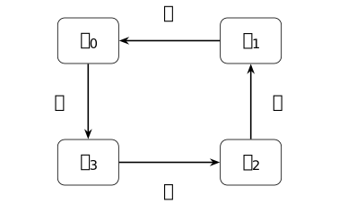
The arrows show the action on basis fields, opposite to the source-to-head orientation on vertices. Every arrow switches support parity; two steps give the half-turn. In particular, over \(\mathbb Z\), \(T^2\delta _0=\delta _2\ne 0\). Thus an odd operator need not square to zero. It need not satisfy a graded commutation law either: that law applied to \(T,T\) would give \(2T^2=0\), whereas \(2T^2\delta _0=2\delta _2\ne 0\).
Identify edge \(i\) with vertex \(i\), with source \(i\) and head \(i+1\), as in Lemma 1.20. Only after this identification does incidence become the endomorphism \(\Delta =T-I\). Its even component is \(-I\) and its odd component is \(T\). Over \(\mathbb Z\), both are nonzero, so \(\Delta \) is inhomogeneous, and \[\Delta ^2\delta _0=\delta _2-2\delta _3+\delta _0\ne 0.\] The formulas remain valid over every commutative unital ring, but the nonzero witnesses just used are specifically over \(\mathbb Z\); in the zero ring all these fields and maps vanish. This is a direct specialization of the shift-multiplication realization and partition construction, not a square-zero differential supplied by parity.
[wieser2022graded, Section 1, accepted-manuscript pp. 1-2] gives the grading convention; the shift, adjoint and failure witnesses are the computations here.
3. Pairings and discrete differences [fdip-0016]AGENTDRAFTED
- October 20, 2026
3. Pairings and discrete differences [fdip-0016]AGENTDRAFTED
- October 20, 2026
How can an edge difference return to a vertex field, and when does its energy detect a constant field? The finite field modules and counting duality give a concrete starting point. Chosen perfect symmetric pairings extend the adjoint construction to different modules over a commutative ring. Applied to incidence, they give weighted energy and the cyclic kinetic factorization.
The component-kernel theorem identifies the additional role of positive real weights; a characteristic-two example shows why perfection alone is insufficient. An invertible precision then gives a unique response to each source, before any probability interpretation.
Definition 3.1. Chosen perfect symmetric pairings [fdip-001O]AGENTDRAFTED
- October 20, 2026
Definition 3.1. Chosen perfect symmetric pairings [fdip-001O]AGENTDRAFTED
- October 20, 2026
The perfect counting duality represents every linear functional by a unique field. To make the same construction on another carrier, let \(R\) be a commutative unital ring and \(M\) a unital \(R\)-module. Write \(M^\vee =\operatorname {Hom}_R(M,R)\) for its dual module. Every linear map here has coefficient map \(\operatorname {id}_R\), as in Remark [ca-001G].
A chosen perfect symmetric pairing on \(M\) is a
bilinear form \(b_M:M\times M\to R\) such that
\(b_M(x,y)=b_M(y,x)\) and the linear map
\[\Phi _M:M\longrightarrow M^\vee ,\qquad
\Phi _M(y)(x)=b_M(x,y)\]
is an isomorphism. Thus each functional \(\ell \)
has exactly one representative \(\Phi _M^{-1}\ell \), characterized by
\(b_M(x,\Phi _M^{-1}\ell )=\ell (x)\) for every \(x\). Bilinearity makes
\(\Phi _M\) linear. Symmetry identifies the other currying map
\(y\mapsto (x\mapsto b_M(y,x))\) with \(\Phi _M\), so both are
isomorphisms. This agrees with the two-sided perfect-pairing convention
in Mathlib's LinearMap.IsPerfPair. The ordinary Hom convention
is [stacks2017stacks, Section 10.10], Tag 0581.
Injectivity alone says that \(b_M(x,y)=0\) for every \(x\) forces \(y=0\); symmetry gives the analogous assertion in the other slot. It does not give every functional a representative; see a zero-radical pairing that is not perfect.
No finiteness, basis or projectivity hypothesis is imposed on \(M\); the specified duality is the assumption. The counting form on every finite function module satisfies it by the explicit inverse in Lemma 2.1. The zero module has its unique perfect pairing. If \(R\) is the zero ring, every unital module is zero since \(x=1x=0x=0\), so this case is included. Perfection does not assert positivity or determine a bilinear form from its diagonal values.
Example 3.2. A zero-radical pairing that is not perfect [fdip-001S]AGENTDRAFTED
- October 20, 2026
Example 3.2. A zero-radical pairing that is not perfect [fdip-001S]AGENTDRAFTED
- October 20, 2026
On the free rank-one \(\mathbb Z\)-module \(M=\mathbb Z\), the symmetric bilinear form \(b(x,y)=2xy\) separates vectors in both slots but is not a perfect pairing. Its currying map is \[\Phi :\mathbb Z\longrightarrow \operatorname {Hom}_{\mathbb Z} (\mathbb Z,\mathbb Z),\qquad \Phi (y)(x)=2xy.\]
If \(b(x,y)=0\) for every integer \(x\), testing against \(x=1\) gives \(2y=0\), hence \(y=0\). Symmetry gives the same conclusion in the other slot, so both radicals are zero and \(\Phi \) is injective. Every integer-linear functional \(\ell \) on \(\mathbb Z\) satisfies \(\ell (x)=x\ell (1)\), so it is determined by its value at \(1\). But \(\Phi (y)(1)=2y\) is even for every \(y\). Thus \(\Phi \) misses the linear functional \(x\mapsto x\), whose value at \(1\) is \(1\), and is not surjective. Freeness of \(M\) does not repair this failure of the chosen form.
The Hom convention is [stacks2017stacks, Section 10.10], Tag 0581; the calculation above proves the failure for this chosen form. For the perfect counting form and its explicit inverse, see Lemma 2.1.
Proposition 3.3. Adjoints from chosen dualities [fdip-001P]AGENTDRAFTED
- October 20, 2026
Proposition 3.3. Adjoints from chosen dualities [fdip-001P]AGENTDRAFTED
- October 20, 2026
Let \(R\) be a commutative unital ring and let \(M,N,P\) be unital \(R\)-modules with chosen perfect symmetric pairings \(b_M,b_N,b_P\) and duality maps \(\Phi _M,\Phi _N,\Phi _P\). For an ordinary \(R\)-linear map \(A:M\to N\), precomposition defines \[A^\vee :N^\vee \longrightarrow M^\vee ,\qquad A^\vee \ell =\ell \circ A.\] Its adjoint for chosen perfect pairings is \[A^\dagger =\Phi _M^{-1}A^\vee \Phi _N:N\longrightarrow M.\] Products denote composition, with the right factor first, as in composition and field multiplication. This is the unique linear map satisfying \[b_M(x,A^\dagger y)=b_N(Ax,y)\qquad (x\in M,\ y\in N).\]
For \(A,A':M\to N\), \(B:N\to P\) and \(r\in R\), \[\begin {aligned} (A+A')^\dagger &=A^\dagger +(A')^\dagger ,& (rA)^\dagger &=rA^\dagger ,\\ 0^\dagger &=0,&I_M^\dagger &=I_M,\\ (BA)^\dagger &=A^\dagger B^\dagger ,& (A^\dagger )^\dagger &=A. \end {aligned}\] If \(A\) is an isomorphism, then \(A^\dagger \) is an isomorphism and \[(A^{-1})^\dagger =(A^\dagger )^{-1}.\] An endomorphism \(L:M\to M\) is self-adjoint for this pairing when \(L^\dagger =L\). In particular, the inverse of an invertible self-adjoint endomorphism is self-adjoint.
Proof.
- October 20, 2026
Proof.
- October 20, 2026
The composite \(\ell \circ A\) is linear. Evaluation at \(x\) gives \[\begin {aligned} A^\vee (\ell +k)(x)&=\ell (Ax)+k(Ax),\\ A^\vee (r\ell )(x)&=r\ell (Ax). \end {aligned}\] Hence \(A^\vee \) is linear, and so is the composite defining \(A^\dagger \). Also \((BA)^\vee =A^\vee B^\vee \) and \(I^\vee =I\), since both sides have the same value on every functional and argument. Because \(\Phi _M\Phi _M^{-1}=I\), \[b_M(x,A^\dagger y)=(A^\vee \Phi _Ny)(x)=b_N(Ax,y).\] If \(K:N\to M\) has the same identity, then \(\Phi _M(Ky)=\Phi _M(A^\dagger y)\) for every \(y\). Injectivity gives \(K=A^\dagger \); existence also used surjectivity of \(\Phi _M\).
Bilinearity shows that \(A^\dagger +(A')^\dagger \), \(rA^\dagger \), \(0\) and \(I_M\) represent the identities for \(A+A'\), \(rA\), \(0\) and \(I_M\), respectively. Uniqueness proves the 4 stated laws. For composition, apply the adjoint identity twice: \[\begin {aligned} b_M(x,A^\dagger B^\dagger z) &=b_N(Ax,B^\dagger z)\\ &=b_P(BAx,z). \end {aligned}\] This proves the product-reversal law. Symmetry gives \[\begin {aligned} b_N(y,Ax)&=b_N(Ax,y)\\ &=b_M(x,A^\dagger y)=b_M(A^\dagger y,x). \end {aligned}\] Thus \(A\) is the adjoint of \(A^\dagger \), proving involution.
Finally, adjointing \(AA^{-1}=I_N\) and \(A^{-1}A=I_M\) gives \[(A^{-1})^\dagger A^\dagger =I_N,\qquad A^\dagger (A^{-1})^\dagger =I_M.\] These are the two inverse identities. If \(A^\dagger =A\), they identify \((A^{-1})^\dagger \) with \(A^{-1}\). No order or division is used.
In particular, for \(d:M\to N\) and a self-adjoint \(W:N\to N\), the composite \(L=d^\dagger Wd:M\to M\) satisfies \[L^\dagger =d^\dagger W^\dagger d=L,\qquad b_M(f,Lg)=b_N(df,Wdg).\] The first equality uses product reversal and double adjunction; the second is the characterizing identity for \(d\). Taking \(g=f\) gives its energy identity, without any order assumption on \(R\).
For a finite function module with its counting form, \(\Phi ^{-1}=\Psi \) from Lemma 2.1; the formula is exactly \(\Psi A^\vee \Phi \) from Proposition 2.4. Hence it gives the same ordinary \(R\)-linear involution on endomorphisms. The proof above extends that direct construction to different carriers.
The Hom convention is [stacks2017stacks, Section 10.10], Tag 0581.
TauCeti's Module.dualEndAlgEquiv expresses
reversed dual composition for reflexive modules. It concerns dual
endomorphisms, before the chosen symmetric identifications used here.
Mathlib's LinearMap.BilinForm.toDual constructs a duality
from a nondegenerate form in the finite-dimensional field case.
Here the dualities are explicitly assumed over \(R\); the argument above
proves the resulting adjoint laws. A nontrivial coefficient involution
and Hermitian forms require different scalar conventions.
Definition 3.4. Weighted graph differentials and adjoints [fdip-0007]AGENTDRAFTED
- October 16, 2026
Definition 3.4. Weighted graph differentials and adjoints [fdip-0007]AGENTDRAFTED
- October 16, 2026
Let \(R\) be a commutative unital ring, \(V,E\) finite sets and \(s,h:E\to V\) endpoint maps. The ring-valued incidence map is \(d_R:H_V\to H_E\), where \(H_V=\mathcal F_R(V)\), \(H_E=\mathcal F_R(E)\) and \(d_Rf(e)=f(h(e))-f(s(e))\). Equip both modules with the symmetric counting forms \[b_V(f,g)=\sum _v f(v)g(v),\qquad b_E(a,c)=\sum _e a(e)c(e).\] Their perfect counting dualities give the counting adjoint \(d_R^\dagger :H_E\to H_V\) by Proposition 3.3. It is characterized by \(b_E(d_Rf,a)=b_V(f,d_R^\dagger a)\).
The return map can be read directly from the endpoints: \[(d_R^\dagger a)(v) =\sum _{h(e)=v}a(e)-\sum _{s(e)=v}a(e).\]
Proof.
- October 16, 2026
Proof.
- October 16, 2026
Expanding and regrouping finite sums gives \[\begin {aligned} b_E(d_Rf,a) &=\sum _e\bigl (f(h(e))-f(s(e))\bigr )a(e)\\ &=\sum _v f(v)\left (\sum _{h(e)=v}a(e)-\sum _{s(e)=v}a(e)\right ). \end {aligned}\] This is the characterizing identity, so uniqueness identifies the map. Each loop occurs once in both sums and cancels; parallel edges remain separate summands. If \(V\) is empty, existence of \(s:E\to V\) forces \(E\) empty; the formula gives the unique map of zero modules.
For arbitrary weights \(w:E\to R\), let \(W:H_E\to H_E\) multiply pointwise by \(w\): \((Wa)(e)=w(e)a(e)\). The weighted graph Laplacian is \[L=d_R^\dagger Wd_R:H_V\longrightarrow H_V.\] Commutativity makes \(W\) self-adjoint, since \(b_E(Wa,c)=\sum _e w(e)a(e)c(e)=b_E(a,Wc)\). The weighted edge form \[b_{E,w}(a,c)=b_E(a,Wc)=\sum _e w(e)a(e)c(e)\] is symmetric bilinear. It is perfect if and only if every \(w(e)\) is a unit, meaning an invertible element of \(R\).
Proof.
- October 16, 2026
Proof.
- October 16, 2026
Its duality map is \(\Phi _EW\). Since \(\Phi _E\) is an isomorphism, \(\Phi _EW\) is an isomorphism exactly when \(W\) is. If every weight is a unit, multiplication by \(w(e)^{-1}\) gives both inverse identities pointwise. Conversely, if \(WJ=I\), evaluate \(WJ\delta _e=\delta _e\) at \(e\): \[w(e)(J\delta _e)(e)=1.\] Commutativity supplies the other inverse identity for this scalar, so \(w(e)\) is a unit. For \(E=\varnothing \), the unit condition is vacuous and \(W\) is the unique isomorphism of the zero module. In the zero ring, \(0=1\) is itself a unit, consistent with the same proof.
Even when some weights are nonunits, the represented return map \(d_R^\dagger W\) exists and satisfies \[b_{E,w}(d_Rf,a)=b_V(f,d_R^\dagger Wa).\] Its existence does not make the weighted edge form perfect. Thus it does not by itself give a two-sided adjoint involution for that form. All these ring identities are direct deductions from the chosen counting dualities. Their positive-real incidence convention is [spielman2009effective, Section 2.1, p. 4].
Orientation reversal leaves \(L\) unchanged. Choose which edges to reverse, and put \(\varepsilon (e)=-1\) on those edges and \(1\) on the others, interpreted in \(R\). The sign map \(Ja(e)=\varepsilon (e)a(e)\) satisfies \(J^\dagger =J\), \(J^2=I\), \(JW=WJ\), and the reversed incidence map is \(d'_R=Jd_R\). Therefore \[(d'_R)^\dagger Wd'_R=d_R^\dagger JWJd_R=d_R^\dagger Wd_R.\] The corresponding edge field is \(a'=Ja\), and \(b_{E,w}(Ja,Jc)=b_{E,w}(a,c)\). The proof includes characteristic two, loops and parallel edges. Endpoints and weights are otherwise fixed.
For the real incidence adapter, start with the incidence map \(D:\mathbb R^V\to \mathbb R^E\) and positive weights \(w(e)>0\). The counting forms are the counting inner products, and write \(D^*=d_{\mathbb R}^\dagger \). The edge form becomes the weighted inner product \[\langle a,c\rangle _{E,w}=\sum _e w(e)a(e)c(e).\] It is symmetric bilinear, and its self-pairing is a finite sum of nonnegative terms. Strictly positive weights make that sum zero only at the zero edge field. Keeping the vertex pairing counting, the weighted adjoint is \(D_w^\dagger =D^*W\), since \[\langle Df,a\rangle _{E,w} =\langle Df,Wa\rangle _E=\langle f,D^*Wa\rangle _V.\] Hence \(L=D^*WD=D_w^\dagger D\); \(D^*D\) is the unit-weight case.
For the coordinate recovery, use the ordered-value isomorphisms \(c_V,c_E\) and incidence matrix \(B=c_EDc_V^{-1}\). The endpoint return formula gives \(c_VD^*c_E^{-1}=B^T\). The multiplication map \(W\) has diagonal array \(\operatorname {diag}(w(e))\); writing the same letter for that array yields \([D_w^\dagger ]=B^TW\) and \([L]=B^TWB\). For a single edge \(0\to 1\) of weight \(c>0\), the two adjoints send an edge value \(a\) to \((-a,a)\) and \((-ca,ca)\), respectively. Under orientation reversal the sign array \(S\) gives \(B'=SB\), \(S^T=S\), \(S^2=I\), \(SWS=W\), and \((B')^TWB'=B^TWB\). A loop has a zero incidence row before and after reversal.
Mathlib's LinearMap.toMatrix_adjoint identifies adjoint
matrices with conjugate transposes in orthonormal bases. Over the reals
this is transpose. The coordinate edge basis is orthonormal for counting,
but not generally for the weighted pairing; the return-map calculation
above accounts for the extra \(W\).
Example 3.5. The weighted four-cycle Laplacian [fdip-004B]AGENTDRAFTED
- October 31, 2026
Example 3.5. The weighted four-cycle Laplacian [fdip-004B]AGENTDRAFTED
- October 31, 2026
Use the alternating four-cycle, with vertices \(0,1,2,3\), edges \(e_i:i\to i+1\), and positive real weights \((1,t,1,t)\). For a field \(f=(a,b,c,d)\), the incidence values are \(Df=(b-a,c-b,d-c,a-d)\). The counting adjoint sends an edge field to \[D^*(u_0,u_1,u_2,u_3) =(u_3-u_0,u_0-u_1,u_1-u_2,u_2-u_3).\] First multiply by \(W_t=\operatorname {diag}(1,t,1,t)\), then apply \(D^*\). The resulting \(L_t=D^*W_tD\) has coordinate matrix \[L_t=\begin {pmatrix} 1+t&-1&0&-t\\ -1&1+t&-t&0\\ 0&-t&1+t&-1\\ -t&0&-1&1+t \end {pmatrix}.\]
For example, its first coordinate is \(t(a-d)-(b-a)=(1+t)a-b-td\); the other coordinates follow from the same return formula. Thus \[L_t\delta _0=(1+t,-1,0,-t),\qquad L_t\mathbf 1=0,\] and the counting energy is \[\langle f,L_tf\rangle =(b-a)^2+t(c-b)^2+(d-c)^2+t(a-d)^2.\] The counting adjoint \(D^*\) does not depend on \(t\). The weighted return map \(D^*W_t\), and hence \(L_t\), do. When \(t=1\) the two return maps coincide; otherwise the factors \(t\) must be retained.
This calculation substitutes the four-cycle data into Definition 3.4; its incidence convention follows [spielman2009effective, Section 2.1, p. 4]. The cyclic energy factorization gives the corresponding operator identity.
Lemma 3.6. Counting adjoints on an indexed cycle [fdip-0014]AGENTDRAFTED
- October 20, 2026
Lemma 3.6. Counting adjoints on an indexed cycle [fdip-0014]AGENTDRAFTED
- October 20, 2026
Let \(R\) be a commutative unital ring. Take the cyclic shift on \(\mathcal F_R(\mathbb Z/n\mathbb Z)\), \(n\ge 1\), with its perfect counting duality \(b\). For the counting adjoint, write \(A^*=A^\dagger \). Then \[T^*=T^{-1},\qquad \Delta ^*=T^{-1}-I.\] Writing \(\nabla ^-=I-T^{-1}\) for the backward difference gives \[\Delta ^*\Delta =-\nabla ^-\Delta =2I-T-T^{-1}.\] Here \(2=1+1\); its invertibility is not required. For the real difference and kinetic signs, see [wingate2025lattice, Section 4, Equations (4.3) and (4.5), p. 3], with lattice spacing one. The finite periodic ring identities follow by reindexing, independently of the product rule.
Proof.
- October 20, 2026
Proof.
- October 20, 2026
The substitution \(j=i+1\) permutes the finite index set, so \[\begin {aligned} b(Tf,g)&=\sum _i f(i+1)g(i)\\ &=\sum _j f(j)g(j-1)=b(f,T^{-1}g). \end {aligned}\] Uniqueness of the counting adjoint gives \(T^*=T^{-1}\). Subtracting \(b(f,g)\) gives \(b(\Delta f,g)=b(f,(T^{-1}-I)g)\), so \(\Delta ^*=T^{-1}-I\). Multiplication gives \[(T^{-1}-I)(T-I)=2I-T-T^{-1}=-\nabla ^-\Delta .\] Consequently \(b(f,\Delta ^*\Delta f)=b(\Delta f,\Delta f)\). Over \(\mathbb R\) this counting form is the counting inner product, and the last expression is \(\sum _i(\Delta f(i))^2\ge 0\).
For the indexed cycle \(e_i:i\to i+1\), the edge-label isomorphism \(j(a)(i)=a(e_i)\) of the cyclic shift and edge-label identification preserves counting pairings: \(b_V(ja,jc)=\sum _i a(e_i)c(e_i)=b_E(a,c)\). Taking \(c=j^{-1}f\) shows that \(j^*=j^{-1}\), hence \(j^*j=I\). Thus \(\Delta =jd_R\) and \[\Delta ^*\Delta =d_R^\dagger j^*j d_R=d_R^\dagger d_R,\] the unit-weight graph Laplacian. At \(n=2\), the two oppositely oriented edges give \(b(f,d_R^\dagger d_Rf)=2(f(1)-f(0))^2\); they are not one simple edge. At \(n=1\), there is one loop, \(T=I\), and both incidence and kinetic maps vanish. An arbitrary incidence map still has distinct vertex and edge carriers; this factorization does not assert that \(\Delta \) is skew-adjoint or square-zero.
Theorem 3.7. Graph energy and the constant modes [fdip-0008]AGENTDRAFTED
- October 16, 2026
Theorem 3.7. Graph energy and the constant modes [fdip-0008]AGENTDRAFTED
- October 16, 2026
Let \(R\) be a commutative unital ring, \(V,E,s,h\) finite incidence data and \(w:E\to R\) arbitrary weights. With the counting forms and weighted graph Laplacian \(L=d_R^\dagger Wd_R\), one has \[L^\dagger =L,\qquad b_V(f,Lg)=\sum _e w(e)(d_Rf)(e)(d_Rg)(e).\] The kernel of \(d_R\) consists exactly of fields constant on each connected component of the underlying undirected graph, and \(\ker d_R\subseteq \ker L\). Two vertices are in the same component when a finite path joins them, with edge orientation ignored.
Proof.
- October 16, 2026
Proof.
- October 16, 2026
The weight map is self-adjoint. The adjoint laws give \(L^\dagger =d_R^\dagger W^\dagger d_R=L\), and the defining identity gives \[\begin {aligned} b_V(f,Lg)&=b_E(d_Rf,Wd_Rg)\\ &=\sum _e w(e)(d_Rf)(e)(d_Rg)(e). \end {aligned}\] In particular, \(b_V(f,Lf)=\sum _e w(e)(d_Rf)(e)^2\). Each edge occurs once and no factor \(1/2\) is used. The equality \(d_Rf=0\) says that endpoint values agree along every edge, hence along every path. Conversely, a componentwise constant field has zero difference on each edge. This identifies \(\ker d_R\) with the function module on the components. Such a field also satisfies \(Lf=d_R^\dagger W0=0\).
The energy is unchanged by edge-orientation reversal: each reversed edge negates both factors in its summand. Equivalently, the orientation-invariant return composite gives the same Laplacian.
Perfection and unit weights do not give the reverse kernel inclusion. Over \(\mathbb F_2\), take two vertices \(0,1\) and two distinct edges, both oriented \(0\to 1\), both of weight \(1\). The counting pairings are perfect and \(W=I\) is invertible. Nevertheless, \[\begin {aligned} d_R(a,b)&=(b-a,b-a),\\ d_R^\dagger (u_1,u_2)&=(-u_1-u_2,u_1+u_2),\\ L(a,b)&=(0,0). \end {aligned}\] For \(\delta _1=(0,1)\), one has \(d_R\delta _1=(1,1)\ne 0\), but its energy is \(1+1=0\). Hence \(\ker L=\mathbb F_2^2\) strictly contains \(\ker d_R=\{(a,a):a\in \mathbb F_2\}\). This failure comes from the absence of real positivity, not from nonunit weights or nonperfect forms.
Now specialize to \(R=\mathbb R\) and \(w(e)>0\). Write \(D=d_{\mathbb R}\). The Laplacian is symmetric and positive semidefinite, and \[\ker L=\ker D,\qquad \dim \ker L=k,\] where \(k\) is the number of connected components. The energy convention and connected-graph argument appear in [spielman2009effective, Section 2.1, pp. 4-5]; the ring identity above and the disconnected, loop and parallel-edge extensions are proved directly here.
Proof.
- October 16, 2026
Proof.
- October 16, 2026
The energy identity specializes to \[\langle f,Lf\rangle _V=\sum _e w(e)(Df)(e)^2\ge 0.\] If \(Lf=0\), this finite sum of nonnegative real terms is zero. Every summand is therefore zero; strict positivity of \(w(e)\) gives \(Df(e)=0\). The reverse inclusion was proved over \(R\). Indicators of the nonempty components span the componentwise constant fields. In a linear relation between them, evaluation at a vertex of any one component makes its coefficient zero. Thus they are a basis, proving the dimension statement. An action defined as half this quadratic form uses a separate convention.
If \(V\) is nonempty and connected, the kernel is the one-dimensional space spanned by the constant field \(\mathbf 1_V\). Its positive unit mode is \[|V|^{-1/2}\mathbf 1_V.\] An isolated vertex contributes one component and one kernel basis vector. If \(V\) is empty, the maps \(s,h:E\to V\) force \(E\) to be empty too: both the component count and kernel dimension are zero. Loops contribute zero energy, while distinct parallel edges each contribute their own positive summand.
For the alternating four-cycle, put \(u=1+t\). Direct multiplication gives \[L_t=\begin {pmatrix} u&-1&0&-t\\ -1&u&-t&0\\ 0&-t&u&-1\\ -t&0&-1&u \end {pmatrix}.\] For \(f=(a,b,c,d)\), the energy is \[\begin {aligned} f^TL_tf={}&(b-a)^2+t(c-b)^2\\ &+(d-c)^2+t(a-d)^2. \end {aligned}\] Every row of \(L_t\) sums to zero, and for \(t>0\) zero energy forces all 4 values equal. The comparison with the positive action identifies how this edge energy combines with a mass term.
The hypotheses have concrete consequences. With vertices \(0,1,2,3\) and just the unit-weight edges \(0\to 1\) and \(2\to 3\), the matrix has two diagonal blocks \(\bigl (\begin {smallmatrix}1&-1\\-1&1\end {smallmatrix}\bigr )\). Its kernel is \(\{(a,a,b,b):a,b\in \mathbb R\}\); connectivity is needed for a single constant mode.
On two vertices with one edge \(0\to 1\) of weight zero, the underlying graph is connected but \(L=0\), so its kernel is all of \(\mathbb R^2\). For nonnegative weights the same proof identifies the kernel using only the positive-weight edges. A zero weight also makes the proposed edge pairing degenerate. If instead this edge has weight \(-1\), then \[f^TLf=-(f(1)-f(0))^2,\] which is negative at \(f=(0,1)\). Positivity fails, and the edge form is not an inner product. This example is negative semidefinite; two disjoint edges with weights \(1\) and \(-1\) give an indefinite form, since fields supported on the separate edges have energies of opposite signs.
For unweighted simple graphs, Mathlib's
SimpleGraph.posSemidef_lapMatrix proves positivity of its
Laplacian. That model has no separate weighted edge set; its energy
formula sums both adjacency directions and divides by two. The
edge-once sum above also handles loops and parallel edges, and is proved
directly here.
Lemma 3.8. Inverse response for an invertible precision [fdip-001Q]AGENTDRAFTED
- October 20, 2026
Lemma 3.8. Inverse response for an invertible precision [fdip-001Q]AGENTDRAFTED
- October 20, 2026
Let \(M\) be a unital module over a commutative unital ring \(R\), with a chosen perfect symmetric pairing \(b\). Let \(L:M\to M\) be self-adjoint, and let \(\mu \in R\). The endomorphism \[Q=L+\mu I_M:M\longrightarrow M\] is self-adjoint. Assume additionally that \(Q\) is an isomorphism, and put \(G=Q^{-1}\). Then \(G^\dagger =G\), and for every source \(j\in M\) the equation \[Qf=j\] has the unique solution \(f=Gj\).
This is a direct consequence of the adjoint and inverse laws and the two-sided inverse convention of [stacks2017stacks, Definition 4.2.4], Tag 0017.
Proof.
- October 20, 2026
Proof.
- October 20, 2026
Linearity of the adjoint and \(I^\dagger =I\) give \(Q^\dagger =L^\dagger +\mu I=Q\). The inverse-adjoint law gives \(G^\dagger =(Q^\dagger )^{-1}=G\). Since \(QG=I\), \(Q(Gj)=j\). Conversely, if \(Qf=j\), then \(GQ=I\) gives \(f=Gj\).
For \(M=\mathcal F_R(V)\) on a finite set with its perfect counting duality, define the point kernel only after this inverse map exists: \[G(v,u)=(G\delta _u)(v).\] The indicator expansion and linearity give \[(Gf)(v)=\sum _{u\in V}G(v,u)f(u).\] Moreover, \[\begin {aligned} G(v,u)&=b(\delta _v,G\delta _u)\\ &=b(G\delta _v,\delta _u)=G(u,v). \end {aligned}\] Thus the symmetric array presents the already defined inverse. On the zero module the unique endomorphism is the identity and is invertible; for an empty carrier the kernel and these sums are empty.
A unit mass coefficient does not ensure invertibility over a ring. Over \(\mathbb Z\), take one unit-weight edge \(0\to 1\), the Laplacian \(L(a,b)=(a-b,b-a)\), and \(\mu =1\). Then \[Q(a,b)=(2a-b,2b-a).\] If \(Q(a,b)=(1,0)\), the second equation gives \(a=2b\), and the first gives \(3b=1\), impossible in \(\mathbb Z\). Thus \(Q\) is not onto, even though the mass and edge weight are units. The real massive Green operator acquires invertibility from positive energy and finite dimension. No positivity, spectrum or probability law is asserted over an arbitrary \(R\).
4. Eliminating a chosen summand [fdip-0020]AGENTDRAFTED
- October 23, 2026
4. Eliminating a chosen summand [fdip-0020]AGENTDRAFTED
- October 23, 2026
When some field values can be solved for, which equation remains on the others? A chosen partition gives one splitting of a field module. More generally, a specified split module and an invertible eliminated component determine a retained linear map. Triangular factorization explains its inverse and kernel before any pairing or probability law is chosen.
Perfect symmetric pairings turn this factorization into a congruence when the splitting is orthogonal. Positive real inner products then give the Schur positivity criterion, and cycle elimination makes the retained inverse comparison explicit. The later Gaussian elimination adds the measure and normalization needed to interpret a retained marginal.
Definition 4.1. Components of a split endomorphism [fdip-001T]AGENTDRAFTED
- October 23, 2026
Definition 4.1. Components of a split endomorphism [fdip-001T]AGENTDRAFTED
- October 23, 2026
To eliminate part of a field, first choose which part is retained. Let \(R\) be a commutative unital ring and \(M,X,Y\) unital \(R\)-modules. A chosen binary splitting of \(M\) consists of ordinary \(R\)-linear maps \[\iota _X:X\to M,\quad \iota _Y:Y\to M,\qquad \pi _X:M\to X,\quad \pi _Y:M\to Y\] satisfying all 5 identities \[\begin {aligned} \pi _X\iota _X&=I_X,&\pi _Y\iota _Y&=I_Y,\\ \pi _X\iota _Y&=0,&\pi _Y\iota _X&=0,\\ \iota _X\pi _X+\iota _Y\pi _Y&=I_M. \end {aligned}\] Products apply the right factor first, as in composition and field multiplication. The maps \((x,y)\mapsto \iota _Xx+\iota _Yy\) and \(z\mapsto (\pi _Xz,\pi _Yz)\) are inverse linear maps by these identities. We consequently write \(M=X\oplus Y\) and \(z=(x,y)\) relative to this chosen identification.
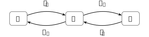
Each summand is included in \(M\) and recovered by its projection. The composite \(\pi _X\iota _X\) is \(I_X\), whereas \(\iota _X\pi _X\) is an endomorphism of \(M\). In the partition realization, these are restriction and extension by zero; the latter composite is the support projection.
For an endomorphism \(Q:M\to M\), its components for the chosen splitting are \[\begin {aligned} A&=\pi _XQ\iota _X:X\to X,&B&=\pi _XQ\iota _Y:Y\to X,\\ E&=\pi _YQ\iota _X:X\to Y,&C&=\pi _YQ\iota _Y:Y\to Y. \end {aligned}\] Inserting \(I_M=\iota _X\pi _X+\iota _Y\pi _Y\) gives \[Q(x,y)=(Ax+By,Ex+Cy).\] If the eliminated component \(C\) is an isomorphism, define the split Schur map, relative to this splitting and pivot, by \[S=A-BC^{-1}E:X\longrightarrow X.\] Changing the splitting or the pivot changes the construction.
The module convention is
[stacks2017stacks, Section 10.10], Tag 0581.
Mathlib's CategoryTheory.Biprod.ofComponents gives
components in a preadditive category with binary biproducts.
Its arguments index source then target; after ordering summands
\((Y,X)\), the arguments corresponding to \(Q\) are \((C,B,E,A)\).
[boyd2004convex, Appendix A.5.5, pp. 650-651] treats the real Schur complement. The source eliminates its first block: exchanging its variables to \((y,x)\) makes its block order \((C,E,B,A)\) and its residual \(A-BC^{-1}E\). The chosen-splitting definition above uses only linear maps; it does not assume a basis, pairing or positivity.
The ring elimination example computes the components and Schur map for a concrete chosen splitting.
Theorem 4.2. Triangular factorization of a split map [fdip-001U]AGENTDRAFTED
- October 23, 2026
Theorem 4.2. Triangular factorization of a split map [fdip-001U]AGENTDRAFTED
- October 23, 2026
Let \(R\) be a commutative unital ring and \(M=X\oplus Y\) a chosen binary splitting of unital \(R\)-modules. Let \(Q(x,y)=(Ax+By,Ex+Cy)\) have the typed components of this splitting, and assume \(C:Y\to Y\) is an isomorphism. Set \[K=C^{-1}E:X\to Y,\qquad S=A-BC^{-1}E:X\to X.\] Define three endomorphisms of \(M\) by \[\begin {aligned} U(x,y)&=(x+BC^{-1}y,y),\\ D(x,y)&=(Sx,Cy),\\ V(x,y)&=(x,y+Kx). \end {aligned}\] Then \(U,V\) are isomorphisms and, with right-factor-first composition, \[Q=UDV.\]
Proof.
- October 23, 2026
Proof.
- October 23, 2026
The displayed maps are linear since every component is linear. Direct substitution on both sides verifies the inverses \[U^{-1}(x,y)=(x-BC^{-1}y,y),\qquad V^{-1}(x,y)=(x,y-Kx).\] These inverses require no inverse of \(S\). Applying the three factors in order gives \[\begin {aligned} DV(x,y)&=(Sx,Ex+Cy),\\ UDV(x,y)&=(Sx+BC^{-1}(Ex+Cy),Ex+Cy)\\ &=(Ax+By,Ex+Cy)=Q(x,y), \end {aligned}\] where \(S+BC^{-1}E=A\) and \(C^{-1}C=I_Y\) give the last equality.
[boyd2004convex, Appendix C.4.1, pp. 672-673] gives real block-system elimination. The proof above extends it directly to modules. The source uses first-pivot order; swapping to the eliminated summand gives the convention here. No finite rank, projectivity or determinant is used.
Mathlib's CategoryTheory.Biprod.gaussian'
supports elimination in a preadditive category with binary biproducts
and an invertible first component. In the order \((Y,X)\), use
\((C,B,E,A)\) as its component arguments. Its notation \(f\gg g\)
applies \(f\) first, so its residual is \(A-BC^{-1}E\).
For finite coordinate index types,
Matrix.fromBlocks_eq_of_invertible₂₂ gives the corresponding
matrix factorization over a commutative ring; its 4 arguments become
\((A,B,E,C)\). These support the factorization, while the subsequent
inverse and kernel
statements have their own proofs.
Theorem 4.3. Inverse components and retained compression [fdip-001V]AGENTDRAFTED
- October 23, 2026
Theorem 4.3. Inverse components and retained compression [fdip-001V]AGENTDRAFTED
- October 23, 2026
Over a commutative unital ring \(R\), let \(M=X\oplus Y\) be a chosen splitting, with ordinary linear endomorphism \(Q(x,y)=(Ax+By,Ex+Cy)\). Assume that the eliminated component \(C\) is an isomorphism, and put \(S=A-BC^{-1}E\). Then \(Q\) is an isomorphism if and only if \(S\) is an isomorphism. When these conditions hold, all 4 components of the inverse are \[\begin {aligned} \pi _XQ^{-1}\iota _X&=S^{-1}:X\to X,\\ \pi _XQ^{-1}\iota _Y&=-S^{-1}BC^{-1}:Y\to X,\\ \pi _YQ^{-1}\iota _X&=-C^{-1}ES^{-1}:X\to Y,\\ \pi _YQ^{-1}\iota _Y&=C^{-1}+C^{-1}ES^{-1}BC^{-1}:Y\to Y. \end {aligned}\] In particular, the retained compression of \(Q^{-1}\) is \(S^{-1}\); it is not in general \(A^{-1}\).
Proof.
- October 23, 2026
Proof.
- October 23, 2026
Use \(Q=UDV\) and the explicit inverses of \(U,V\) from triangular factorization, where \(D(x,y)=(Sx,Cy)\). If \(S\) is invertible, then \(D^{-1}(u,v)=(S^{-1}u,C^{-1}v)\). Thus \(Q^{-1}=V^{-1}D^{-1}U^{-1}\) is a two-sided inverse.
Conversely, suppose \(Q\) is invertible. Then \(D=U^{-1}QV^{-1}\) is invertible; write \(J=D^{-1}\) and set \(J_X=\pi _XJ\iota _X:X\to X\). The identities \(\pi _XD=S\pi _X\) and \(D\iota _X=\iota _XS\) imply \[\begin {aligned} SJ_X&=\pi _XDJ\iota _X=\pi _X\iota _X=I_X,\\ J_XS&=\pi _XJD\iota _X=\pi _X\iota _X=I_X. \end {aligned}\] Hence \(J_X\) is a two-sided inverse of \(S\). This implication still uses the assumed invertibility of \(C\).
Applying the three inverse factors to \((u,v)\) gives \[\begin {aligned} x&=S^{-1}u-S^{-1}BC^{-1}v,\\ y&=-C^{-1}ES^{-1}u +(C^{-1}+C^{-1}ES^{-1}BC^{-1})v. \end {aligned}\] Setting one input component to zero and projecting the other gives the 4 stated map identities.
The real symmetric inverse formula is
[boyd2004convex, Appendix A.5.5, p. 650]; its first-pivot
convention is exchanged here. The direct proof uses arbitrary unital
\(R\)-modules and needs no pairing or symmetry.
Mathlib's CategoryTheory.Biprod.isoElim' constructs
the residual isomorphism when both the first component and the whole
biproduct map are isomorphisms. With summands \((Y,X)\) and component
arguments \((C,B,E,A)\), it supports the whole-to-residual direction;
it does not by itself assert the 4 inverse formulas above.
For a self-adjoint precision with a chosen perfect pairing, inverse response supplies its separate response interpretation. The cycle calculation exhibits a retained inverse entry \(2/15\) where \(A^{-1}\) has entry zero. No probability law is needed for the map comparison.
Proposition 4.4. Eliminating equations and identifying kernels [fdip-001W]AGENTDRAFTED
- October 23, 2026
Proposition 4.4. Eliminating equations and identifying kernels [fdip-001W]AGENTDRAFTED
- October 23, 2026
Let \(R\) be a commutative unital ring and choose \(M=X\oplus Y\) with components \(Q(x,y)=(Ax+By,Ex+Cy)\). Assume \(C:Y\to Y\) is an isomorphism and set \(S=A-BC^{-1}E\). For every \(u\in X,v\in Y\), \[Q(x,y)=(u,v)\] is equivalent to the two equations \[y=C^{-1}(v-Ex),\qquad Sx=u-BC^{-1}v.\] No invertibility of \(S\) is required. In particular, the maps \[\begin {aligned} J_S:\ker S&\longrightarrow \ker Q,& x&\longmapsto (x,-C^{-1}Ex),\\ \pi _X:\ker Q&\longrightarrow \ker S,& (x,y)&\longmapsto x \end {aligned}\] are inverse \(R\)-linear maps. Here each kernel is the submodule of elements sent to zero.
Proof.
- October 23, 2026
Proof.
- October 23, 2026
The second component of \(Q(x,y)=(u,v)\) is \(Ex+Cy=v\); since \(C\) is invertible, it is equivalent to \(y=C^{-1}(v-Ex)\). Substitution in \(Ax+By=u\) gives \[Ax+BC^{-1}(v-Ex)=Sx+BC^{-1}v=u.\] Reversing these steps proves the full equivalence.
For any \(x\in X\), direct substitution gives \[Q(x,-C^{-1}Ex)=(Sx,0).\] Thus \(J_S\) sends \(\ker S\) into \(\ker Q\). If \(Q(x,y)=0\), the proved equivalence gives \(Sx=0\) and \(y=-C^{-1}Ex\). Therefore \(\pi _XJ_Sx=x\) and \(J_S\pi _X(x,y)=(x,y)\) on the stated kernels. Both maps are restrictions of linear maps, so this is a module isomorphism, not merely a bijection of sets.
[boyd2004convex, Appendix C.4.1, pp. 672-673] gives real linear-system elimination. The direct argument above extends it to modules. After exchanging the source variables to \((y,x)\) and the right side to \((v,u)\), its first-pivot equations become the displayed formulas. The kernel correspondence does not assume that the whole system is invertible.
The pivot hypothesis cannot be deduced from invertibility of \(Q\). Over a nonzero ring take \(X=Y=R\) and \(Q(x,y)=(y,x)\). Then \(Q^2=I\), but its component \(C=0:R\to R\) is not an isomorphism. These formulas cannot invert that prescribed pivot.
Zero summands cause no exception. If \(Y=0\), its unique endomorphism is its identity and is invertible; then \(S=A\) and elimination changes nothing. If \(X=0\), \(S\) is the unique invertible endomorphism of zero and \(Q=C\). Over the zero ring every unital module is zero, because \(x=1x=0x=0\); all statements remain valid.
Proposition 4.5. Elimination with orthogonal perfect pairings [fdip-001X]AGENTDRAFTED
- October 23, 2026
Proposition 4.5. Elimination with orthogonal perfect pairings [fdip-001X]AGENTDRAFTED
- October 23, 2026
Let \(X,Y\) be unital modules over a commutative unital ring \(R\), with chosen perfect symmetric pairings \(b_X,b_Y\). On the chosen sum \(M=X\oplus Y\), choose the orthogonal sum form \[b_M((x,y),(x',y'))=b_X(x,x')+b_Y(y,y').\] It is perfect and symmetric, and its injection/projection adjoints are \[\iota _X^\dagger =\pi _X,\quad \pi _X^\dagger =\iota _X,\qquad \iota _Y^\dagger =\pi _Y,\quad \pi _Y^\dagger =\iota _Y.\] Suppose \(Q:M\to M\) is self-adjoint, with components \(A,B,E,C\) and invertible \(C\). Then \[A^\dagger =A,\quad C^\dagger =C,\quad E=B^\dagger ,\qquad S^\dagger =S\quad \text {for }S=A-BC^{-1}E.\] For the triangular factors, \[V^\dagger =U,\qquad Q=V^\dagger DV,\qquad D(x,y)=(Sx,Cy).\] Consequently, with \(K=C^{-1}E\), \[\begin {aligned} b_M((x,y),Q(x,y)) &=b_X(x,Sx)\\ &\quad +b_Y(y+Kx,C(y+Kx)). \end {aligned}\]
Proof.
- October 23, 2026
Proof.
- October 23, 2026
Bilinearity and symmetry of \(b_M\) follow termwise. For a linear functional \(\ell :M\to R\), represent \(\ell \iota _X\) and \(\ell \iota _Y\) uniquely by \(x_\ell \in X,y_\ell \in Y\) using the two perfect pairings. Then for every \((x,y)\), \[\ell (x,y)=\ell \iota _X(x)+\ell \iota _Y(y) =b_X(x,x_\ell )+b_Y(y,y_\ell ).\] This gives a representative \((x_\ell ,y_\ell )\). Uniqueness follows by testing \((x,0)\) and \((0,y)\) separately. The representative depends linearly on \(\ell \), since the two inverse duality maps are linear. Thus the currying map of \(b_M\) is a linear isomorphism.
For example, \(b_M(\iota _Xx,(u,v))=b_X(x,u)=b_X(x,\pi _X(u,v))\). Adjoint uniqueness and involution give the two \(X\) identities, and the same calculation gives those for \(Y\). Adjointing the definitions of the 4 components and using \(Q^\dagger =Q\) gives \(A^\dagger =A\), \(C^\dagger =C\) and \(B^\dagger =E\). The inverse-adjoint law then gives \((C^{-1})^\dagger =C^{-1}\) and \[K^\dagger =(C^{-1}E)^\dagger =BC^{-1},\qquad (BC^{-1}E)^\dagger =BC^{-1}E.\] The latter identity proves \(S^\dagger =S\).
For \(z=(x,y)\) and \(w=(u,v)\), \[\begin {aligned} b_M(Vz,w) &=b_X(x,u)+b_Y(y+Kx,v)\\ &=b_X(x,u+K^\dagger v)+b_Y(y,v)\\ &=b_M(z,Uw). \end {aligned}\] Uniqueness gives \(V^\dagger =U\); factorization yields \(Q=V^\dagger DV\). Finally \(b_M(z,Qz)=b_M(Vz,DVz)\), and expanding the orthogonal sum form gives the stated identity.
This is a direct deduction from chosen dualities and triangular factorization. The real symmetric completion in [boyd2004convex, Appendix A.5.5, p. 650] is its real coordinate specialization. The chosen orthogonal sum is essential: an arbitrary perfect form on \(M\) need not have these injection/projection adjoints. No division by two or recovery of bilinear data from diagonal values is used; the identity remains valid in characteristic two.
TauCeti's LinearMap.BilinForm.prod gives the
orthogonal product form, and
LinearMap.BilinForm.nondegenerate_prod_iff identifies
its radical nondegeneracy. The functional-splitting proof above also
proves the surjectivity required for perfection. These declarations
alone do not assert the paired-congruence result.
Proposition 4.6. Positive definiteness under elimination [fdip-001Y]AGENTDRAFTED
- October 23, 2026
Proposition 4.6. Positive definiteness under elimination [fdip-001Y]AGENTDRAFTED
- October 23, 2026
Let \(X,Y\) be finite-dimensional real vector spaces with positive definite inner products \(b_X,b_Y\). Give \(M=X\oplus Y\) their orthogonal sum, and let \(Q:M\to M\) be self-adjoint, with components \(A,B,E,C\). For a self-adjoint map \(T\) on any of these spaces, write \(T>0\) when \(b(z,Tz)>0\) for every nonzero \(z\).
If \(Q>0\), then \(C\) is positive definite and invertible, and \(S=A-BC^{-1}E\) is positive definite and invertible. Conversely, if \(C\) is invertible, then \[Q>0\quad \Longleftrightarrow \quad C>0\ \text {and}\ S>0.\]
[boyd2004convex, Appendix A.5.5, p. 650] gives the positive-definite Schur criterion. Here the eliminated summand is placed second.
Proof.
- October 23, 2026
Proof.
- October 23, 2026
The currying map of each inner product is injective. Indeed, if \(b(z,u)=0\) for every \(z\), take \(z=u\); positive definiteness gives \(u=0\). Finite dimension makes this map onto the dual, which has the same dimension. Thus these forms are chosen perfect pairings, and the paired-congruence identity applies whenever \(C\) is invertible.
Assume \(Q>0\). For \(y\ne 0\), \(\iota _Yy\ne 0\) and \[b_Y(y,Cy)=b_M(\iota _Yy,Q\iota _Yy)>0.\] Hence \(C>0\). If \(Cy=0\), positivity forces \(y=0\); finite dimension then turns injectivity into surjectivity, so \(C\) is invertible. For \(x\ne 0\), the vector \((x,-C^{-1}Ex)\) is nonzero and congruence gives \[b_X(x,Sx) =b_M((x,-C^{-1}Ex),Q(x,-C^{-1}Ex))>0.\] Thus \(S>0\), and the same injectivity and finite-dimension argument makes \(S\) invertible.
Conversely, suppose \(C>0\) and \(S>0\). For any nonzero \(z=(x,y)\), the invertible map \(V(x,y)=(x,y+C^{-1}Ex)\) has \(Vz\ne 0\). At least one of its two components is nonzero. The corresponding term of \[b_M(z,Qz)=b_X(x,Sx)+b_Y(y+C^{-1}Ex,C(y+C^{-1}Ex))\] is strictly positive, and the other is nonnegative. Hence \(Q>0\). If a summand is zero, its positivity assertion is vacuous and its unique endomorphism is invertible, so the same argument includes it.
This uses finite-dimensional real positivity in addition to the ring-level factorization. It explains the positivity assumption in real effective precision. It does not evaluate an integral or determine a normalization factor; those require the separately specified real measure and Gaussian law.
Example 4.7. Eliminating alternate vertices of a ring-valued cycle [fdip-001Z]AGENTDRAFTED
- October 23, 2026
Example 4.7. Eliminating alternate vertices of a ring-valued cycle [fdip-001Z]AGENTDRAFTED
- October 23, 2026
Use the four-cycle endpoints \(s(e_i)=i\), \(h(e_i)=i+1\) on \(\mathbb Z/4\mathbb Z\), but now let \(R\) be any commutative unital ring and take \(t,\mu \in R\). Give successive edges weights \((1,t,1,t)\). On the finite function modules with their counting pairings, set \[Q=d^\dagger Wd+\mu I,\qquad s=1+t+\mu .\] Here \(d\) is incidence and \(W\) multiplies each edge field by its weight. This extends the positive-real weight choice in Example 1.8; no weight is assumed positive or invertible.
First compute from endpoints. The difference is \((df)(e_i)=f(i+1)-f(i)\). Grouping the incoming and outgoing edge terms gives \[(d^\dagger Wdf)(i) =w(e_{i-1})(f(i)-f(i-1))+w(e_i)(f(i)-f(i+1)).\] Adding \(\mu f(i)\) yields \[\begin {aligned} (Qf)(0)&=sf(0)-f(1)-tf(3),\\ (Qf)(1)&=sf(1)-f(0)-tf(2),\\ (Qf)(2)&=sf(2)-tf(1)-f(3),\\ (Qf)(3)&=sf(3)-tf(0)-f(2). \end {aligned}\]
Choose the additional partition \(V_0=\{0,2\}\), \(V_1=\{1,3\}\), and put \(X=\mathcal F_R(V_0)\), \(Y=\mathcal F_R(V_1)\). Restriction and extension by zero give the chosen splitting. The resulting component maps are \[\begin {aligned} A&=sI_X,&C&=sI_Y,\\ (Ex)(1)&=-x(0)-tx(2),&(Ex)(3)&=-tx(0)-x(2),\\ (By)(0)&=-y(1)-ty(3),&(By)(2)&=-ty(1)-y(3). \end {aligned}\] The pivot \(C\) is invertible exactly when \(s\) is a unit. A unit gives \(C^{-1}=s^{-1}I_Y\). Conversely, if \(CJ=I_Y\), evaluation of \(CJ\delta _1=\delta _1\) at vertex \(1\) gives \(s(J\delta _1)(1)=1\); commutativity makes this a two-sided inverse of \(s\). In the zero ring \(0=1\) is a unit, consistently with this argument.
Assume this unit condition. Applying \(B\) to \(Ex\) gives \[\begin {aligned} (BEx)(0)&=(1+t^2)x(0)+2tx(2),\\ (BEx)(2)&=2tx(0)+(1+t^2)x(2). \end {aligned}\] Consequently the split Schur map is \[\begin {aligned} (Sx)(0)&=[s-s^{-1}(1+t^2)]x(0)-2ts^{-1}x(2),\\ (Sx)(2)&=[s-s^{-1}(1+t^2)]x(2)-2ts^{-1}x(0). \end {aligned}\] Here \(2=1+1\); neither \(2\), \(t\), \(\mu \) nor \(S\) is asserted to be invertible. In coordinates ordered \((0,2)\), the same map is \[[S]=\begin {pmatrix} s-s^{-1}(1+t^2)&-2ts^{-1}\\ -2ts^{-1}&s-s^{-1}(1+t^2) \end {pmatrix}.\] This array presents the map just computed from endpoints.
The half-turn exchanges \(0\leftrightarrow 2\) and \(1\leftrightarrow 3\). Let \(r_X,r_Y\) exchange the corresponding field values. The component formulas give \(Ar_X=r_XA\), \(Cr_Y=r_YC\), \(Er_X=r_YE\) and \(Br_Y=r_XB\); hence \(Sr_X=r_XS\). A one-step shift exchanges the two parts and fails to preserve the alternating weights when \(t\ne 1\). No retained partition is implicit in general incidence data.
Now specialize to \(R=\mathbb R\), \(t>0\), \(\mu =m^2>0\). The weighted energy identity gives, for \(f\ne 0\), \[b(f,Qf)=\sum _e w(e)(df(e))^2+m^2\sum _v f(v)^2>0.\] Thus \(Q\) is positive definite and invertible, and the positive-real criterion gives \(S>0\). At \(t=m=1\), \(s=3\) and \[[S]=\frac 13\begin {pmatrix}7&-2\\-2&7\end {pmatrix}.\] To solve \(Sx=\delta _2\), solve \(7x(0)-2x(2)=0\) and \(-2x(0)+7x(2)=3\). These give \(x(2)=7/15\) and \(x(0)=2/15\). Therefore \[(\pi _XQ^{-1}\iota _X\delta _2)(0) =(S^{-1}\delta _2)(0)=\frac {2}{15}.\] By contrast, fixing the eliminated field to zero leaves the retained map \(A=3I_X\), and \((A^{-1}\delta _2)(0)=0\). These are different map operations.
At real \(\mu =0,t>0\), the pivot \(C=(1+t)I_Y\) is still invertible. But \(s-s^{-1}(1+t^2)=2t/(1+t)\), so the nonzero constant retained field satisfies \(S1=0\). The kernel correspondence then recovers the constant full field in \(\ker Q\), since \(-C^{-1}E1=1\). An invertible pivot does not imply an invertible full precision.
[spielman2009effective, Section 2.1, pp. 4-5] gives the incidence sign convention for positive real weights. The arbitrary-ring identities use the direct counting construction of Definition 3.4.
[boyd2004convex, Appendix C.4.1, pp. 672-673] gives the real elimination convention. All coefficients and inverse entries here were computed from the specified endpoints and weights. They recover the algebraic values in real alternate-vertex elimination; the covariance and marginal-law interpretation there additionally uses the Gaussian measure. No massless Gaussian formula follows by substituting \(\mu =0\) into a massive normalization.
How do we describe fields other than a distinguished solution? In the finite real specialization with counting inner product and symmetric positive-definite precision \(Q\), a source \(j\) singles out \(f=Q^{-1}j\), the unique solution of \(Qf=j\). Completing the square also makes it the minimizer of \(f^TQf-2j^Tf\). This extra positivity does not belong to the general ring-level elimination above. Even in this case, a solution does not specify probabilities for other fields. Statistical fluctuations require a law and the expected values of observables. The next chapter starts with a finite law; reference measure and Gaussian integrability later make that question precise for real-valued fields.
5. States and pullback of observables [fdip-002B]AGENTDRAFTED
- October 23, 2026
5. States and pullback of observables [fdip-002B]AGENTDRAFTED
- October 23, 2026
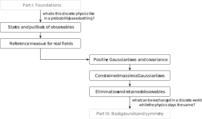
How can a model describe many possible fields and average what we observe? A law on a finite set of configurations assigns probability weights to those fields and averages their observables. The 16 binary fields on the four-cycle give a concrete example: summing weights over configurations with the same retained values produces the retained law. These probability weights are chosen independently of the edge energies. Real probability weights on binary fields are distinct from real-valued field coordinates. Observable algebras and normalized functionals express this operation without assuming a finite configuration set.
A supplied algebra map pulls a functional back by precomposition. Over the reals or complexes, positivity and the involution determine which functionals are states; the real dual-number example explains why the hypotheses matter. Coordinate restriction then pulls polynomial observables back. For real fields with infinitely many configurations, reference measure and Gaussian integrability give the corresponding expectations.
Definition 5.1. Normalized linear functionals [fdip-0021]AGENTDRAFTED
- October 23, 2026
Definition 5.1. Normalized linear functionals [fdip-0021]AGENTDRAFTED
- October 23, 2026
Let \(R\) be a commutative unital ring, allowing \(1=0\), and let \(A\) be a unital associative algebra over \(R\). Its scalar map is \(\eta :R\to A\), \(r\mapsto r1_A\), with central image. A normalized linear functional is an ordinary \(R\)-linear map \(\omega :A\to R\) satisfying \(\omega (1_A)=1_R\). Thus \(\omega (ra+sb)=r\omega (a)+s\omega (b)\); the coefficient map for linearity is \(\mathrm {id}_R\), not a nontrivial semilinear twist. This is a member of the dual module, with an additional normalization condition.
Normalization is equivalent to \(\omega \circ \eta =\mathrm {id}_R\). In particular, a normalized functional can exist only if \(\eta \) is injective. This necessary condition alone is not a claim of existence.
Proof.
- October 23, 2026
Proof.
- October 23, 2026
If \(\omega (1_A)=1_R\), linearity gives \(\omega (\eta (r))=\omega (r1_A)=r\omega (1_A)=r\). Conversely, evaluating \(\omega \eta =\mathrm {id}_R\) at \(1_R\) gives \(\omega (1_A)=1_R\). A map with a left inverse is injective.
For example, the scalar map \(\mathbb Z\to \mathbb Z/2\mathbb Z\) is not injective, so this algebra admits no normalized \(\mathbb Z\)-linear functional. If \(A\) is the zero algebra, normalization is possible exactly when \(R\) is the zero ring. If \(R\) is the zero ring, every unital \(R\)-module is zero, since \(a=1_Ra=0_Ra=0\); its unique functional is normalized.
The algebra conventions are those of
[stacks2017stacks, Section 22.2], Tag 09JF and
[jadczyk2019notes, Definition 1.6, p. 4].
Mathlib's Module.Dual supplies the ordinary linear dual;
normalization and the scalar left-inverse criterion are the additional
conditions proved here. No order, involution or topology is part of this definition.
Example 5.2. Observables on a finite configuration set [fdip-0022]AGENTDRAFTED
- October 23, 2026
Example 5.2. Observables on a finite configuration set [fdip-0022]AGENTDRAFTED
- October 23, 2026
Let \(V\) be a finite vertex set and \(S\) a finite set of possible values. A configuration is a function \(\sigma :V\to S\); the configuration set is \(\Omega =S^V\). The set \(\Omega \) is distinct from the vertex set \(V\): an observable takes a whole configuration as its input. For a commutative unital ring \(R\), set \[A_\Omega =\operatorname {Map}(\Omega ,R).\] This is the pointwise function algebra: \((f+g)(\sigma )=f(\sigma )+g(\sigma )\), \((fg)(\sigma )=f(\sigma )g(\sigma )\) and \((rf)(\sigma )=rf(\sigma )\), with unit the constant function \(1_R\).
For each \(\sigma \in \Omega \), evaluation \(\operatorname {ev}_\sigma (f)=f(\sigma )\) is a unital \(R\)-algebra map and a normalized linear functional. The scalar map sends \(r\) to the constant function \(r\). The indicator \(\delta _\sigma \) is \(1_R\) at \(\sigma \) and \(0_R\) elsewhere. These are the same indicators used in counting duality for finite functions, now indexed by configurations.
Proof.
- October 23, 2026
Proof.
- October 23, 2026
Each algebra law follows by evaluating at every configuration and using the corresponding law in \(R\). Evaluation preserves addition, scalar multiplication, products and the unit by the displayed definitions. The indicators satisfy \[\delta _\sigma ^2=\delta _\sigma ,\qquad \delta _\sigma \delta _\tau =0\ (\sigma \ne \tau ),\qquad \sum _{\sigma \in \Omega }\delta _\sigma =1.\] These equalities hold pointwise, including when \(R\) is the zero ring.
If \(V=\varnothing \), then \(S^V\) contains the unique empty function, even when \(S=\varnothing \). If \(S=\varnothing \) and \(V\ne \varnothing \), then \(\Omega =\varnothing \); its function algebra is the zero algebra. There is then no evaluation at a configuration.
The underlying unital algebra convention is
[stacks2017stacks, Section 22.2], Tag 09JF.
Mathlib's Pi.algebra, Pi.evalAlgHom and
Pi.constAlgHom provide the pointwise algebra, evaluation and
constant algebra maps. The configuration interpretation and the empty-set
cases above are direct consequences of these definitions.
Proposition 5.3. Finite functionals and their weights [fdip-0023]AGENTDRAFTED
- October 23, 2026
Proposition 5.3. Finite functionals and their weights [fdip-0023]AGENTDRAFTED
- October 23, 2026
For a finite set \(\Omega \) and commutative unital ring \(R\), every \(R\)-linear functional on the function algebra has a unique weight function \(p:\Omega \to R\), given by \[\omega (f)=\sum _{x\in \Omega }p(x)f(x),\qquad p(x)=\omega (\delta _x).\] Conversely, every such weight function defines an \(R\)-linear functional. It is normalized exactly when \(\sum _xp(x)=1_R\).
Proof.
- October 23, 2026
Proof.
- October 23, 2026
Pointwise evaluation gives \(f=\sum _x f(x)\delta _x\). Linearity therefore gives the stated formula, using commutativity of \(R\) to write the coefficients in either order. Conversely, distributivity of the finite sum proves linearity of the formula. Evaluating it on \(\delta _y\) recovers \(p(y)\), proving uniqueness in both directions. Evaluating at \(1=\sum _x\delta _x\) proves the normalization criterion.
When \(\Omega =\varnothing \), the sole functional is the zero map from the zero algebra and its total weight is \(0_R\); it is normalized exactly when \(R\) is the zero ring. When \(\Omega \ne \varnothing \), a chosen evaluation is normalized over every \(R\). Uniform weights \(p(x)=c\) on a set of size \(n>0\) are normalized exactly when \((n1_R)c=1_R\). Such normalized uniform weights exist exactly when \(n1_R\) is a unit, and then the unique coefficient is \(c=(n1_R)^{-1}\). Thus failure of uniform normalization does not imply failure of all normalized functionals.
More generally, for raw weights \(w(x)\) with total \(Z=\sum _xw(x)\), a common rescaling \(p(x)=cw(x)\) is normalized exactly when \(cZ=1_R\). This is possible exactly when \(Z\) is a unit, and then \(c=Z^{-1}\) is unique. No division by a nonunit is defined by this formula. In the zero ring the sole element is a unit, so the same criterion applies. For real nonnegative weights, \(Z>0\) exactly when at least one weight is positive; all-zero weights cannot be normalized by rescaling.
This is the indicator-basis argument of finite function duality, with the unital algebra convention of [stacks2017stacks, Section 22.2], Tag 09JF. For real nonnegative normalized weights it gives the finite expectation. No positivity or division is needed for the ring-valued classification.
Definition 5.4. Real and complex algebraic states [fdip-0024]AGENTDRAFTED
- October 23, 2026
Definition 5.4. Real and complex algebraic states [fdip-0024]AGENTDRAFTED
- October 23, 2026
Let \(K=\mathbb R\) or \(K=\mathbb C\), with conjugation the identity in the real case. Let \(A\) be a unital associative \(K\)-algebra equipped with an additive operation \(a\mapsto a^*\) satisfying \[\begin {aligned} (\lambda a)^*&=\overline \lambda a^*,& (ab)^*&=b^*a^*,\\ (a^*)^*&=a,&1^*&=1. \end {aligned}\] There is no graded sign in the product law. A \(K\)-linear functional \(\omega :A\to K\) is Hermitian positive when \[\omega (a^*)=\overline {\omega (a)},\qquad \omega (a^*a)\in \mathbb R_{\geq 0}\quad (a\in A).\] A real algebraic state, respectively a complex algebraic state, is such a functional that is also normalized. The scalar field and involution are part of the assertion.
Over \(\mathbb C\), nonnegativity on all \(a^*a\) already implies Hermiticity, without assuming normalization. Over \(\mathbb R\), Hermiticity is a separate requirement, as the real dual-number example shows.
Proof.
- October 23, 2026
Proof.
- October 23, 2026
Suppose \(K=\mathbb C\) and \(\omega (a^*a)\in \mathbb R_{\geq 0}\) for every \(a\). For \(h=h^*\), expansion and linearity give \[\begin {aligned} 4\omega (h)={}&\omega ((1+h)^*(1+h))\\ &-\omega ((1-h)^*(1-h))\in \mathbb R. \end {aligned}\] For arbitrary \(a\), put \(h=(a+a^*)/2\) and \(k=(a-a^*)/(2i)\). Conjugate scalar compatibility gives \(h=h^*\), \(k=k^*\), \(a=h+ik\) and \(a^*=h-ik\). The preceding calculation makes \(\omega (h)\) and \(\omega (k)\) real. Hence \(\omega (a^*)=\omega (h)-i\omega (k)=\overline {\omega (a)}\).
For these conventions, see [waldmann2004states, Section 3.1, p. 9; Definition 3.7 and Definition 3.9 with Remark 3.10(iv), p. 11]. Waldmann works over a complexification of an ordered ring. Here the coefficients are the ordinary fields \(\mathbb R\) and \(\mathbb C\); the real Hermiticity requirement is explicit. On p. 9, Definition 3.1 prints \(R=-P\sqcup \{0\}\sqcup R\); the intended final \(P\), rather than the printed \(R\), is a mathematical emendation, not a verbatim transcription.
The ordinary linear involution is not a substitute for conjugate scalar compatibility over \(\mathbb C\). With a complex-linear unital involution, \((i1)^*(i1)=-1\); a normalized functional takes this to \(-1\), contradicting square positivity. The earlier chosen bilinear adjoints likewise do not supply this Hermitian structure. No norm, continuity or operator representation is assumed.
Example 5.5. Square positivity need not imply real Hermiticity [fdip-0025]AGENTDRAFTED
- October 23, 2026
Example 5.5. Square positivity need not imply real Hermiticity [fdip-0025]AGENTDRAFTED
- October 23, 2026
In the real algebra \(A=\mathbb R[\varepsilon ]/(\varepsilon ^2)\), each element is uniquely \(x+y\varepsilon \). Define \((x+y\varepsilon )^*=x-y\varepsilon \). For any fixed real \(c\ne 0\), let \[\omega _c(x+y\varepsilon )=x+cy.\] Then \(\omega _c\) is normalized and nonnegative on every \(a^*a\), but is not a real algebraic state, because it is not Hermitian.
Proof.
- October 23, 2026
Proof.
- October 23, 2026
The operation is real linear, fixes the unit and squares to the identity. Multiplication gives \((x+y\varepsilon )(u+v\varepsilon )=xu+(xv+yu)\varepsilon \); applying star negates the second coefficient, as does multiplying the starred factors. Since the algebra is commutative, this is also the required order-reversing product law. For \(a=x+y\varepsilon \), \(a^*a=(x-y\varepsilon )(x+y\varepsilon )=x^2\). Thus \(\omega _c(a^*a)=x^2\geq 0\), and \(\omega _c(1)=1\). But \(\omega _c(\varepsilon ^*)=-c\ne c=\omega _c(\varepsilon )\).
This direct calculation distinguishes square positivity from the extra real Hermiticity condition. Square positivity is defined in [waldmann2004states, Definition 3.9, p. 11]. It is separate from the characteristic-two group-algebra example: the present algebra and functional are over \(\mathbb R\).
Proposition 5.6. Finite states are probability weights [fdip-0026]AGENTDRAFTED
- October 23, 2026
Proposition 5.6. Finite states are probability weights [fdip-0026]AGENTDRAFTED
- October 23, 2026
Let \(\Omega \) be finite, \(K=\mathbb R\) or \(\mathbb C\), and give \(A_\Omega =\operatorname {Map}(\Omega ,K)\) the pointwise involution \(f^*(x)=\overline {f(x)}\). The weight functional \(\omega _p(f)=\sum _xp(x)f(x)\) is a real or complex algebraic state exactly when every \(p(x)\) is real and nonnegative and \(\sum _xp(x)=1\).
Proof.
- October 23, 2026
Proof.
- October 23, 2026
Pointwise conjugation is additive, conjugates scalars, fixes the unit and is involutive. It reverses products because \(K\) is commutative. For necessity, \(\delta _x^*\delta _x=\delta _x\), so square positivity gives \(p(x)=\omega _p(\delta _x)\in \mathbb R_{\geq 0}\). Normalization gives the sum condition. Conversely, real weights imply \(\omega _p(f^*)=\sum _xp(x)\overline {f(x)}=\overline {\omega _p(f)}\). Furthermore \[\omega _p(f^*f)=\sum _xp(x)|f(x)|^2\geq 0,\] and \(\omega _p(1)=\sum _xp(x)=1\). For a real pointwise nonnegative function, each summand \(p(x)f(x)\) is also nonnegative, so its expectation is nonnegative.
There is no state on the empty configuration set over \(\mathbb R\) or \(\mathbb C\), because the empty sum is zero. On two points, the weights \(p(0)=p(1)=1/2\) give a state that is not multiplicative: \(\omega _p(\delta _0\delta _1)=0\), whereas \(\omega _p(\delta _0)\omega _p(\delta _1)=1/4\). A state is not required to be an algebra homomorphism.
The positive-functional convention is [waldmann2004states, Definition 3.9, p. 11]; the indicator calculation above identifies it with finite probability and expectation on this particular algebra. It does not identify positivity cones on arbitrary star algebras; the distinctions on [waldmann2004states, p. 12] remain separate.
Proposition 5.7. Pulling a functional back along a supplied algebra map [fdip-0027]AGENTDRAFTED
- October 23, 2026
Proposition 5.7. Pulling a functional back along a supplied algebra map [fdip-0027]AGENTDRAFTED
- October 23, 2026
Let \(R\) be a commutative unital ring, \(A,B\) unital associative \(R\)-algebras, and let \(\iota :B\to A\) be a supplied unital algebra homomorphism. Precomposition defines an \(R\)-linear map in the opposite direction on ordinary duals: \[\begin {aligned} \iota ^\flat :\operatorname {Hom}_R(A,R)&\longrightarrow \operatorname {Hom}_R(B,R),\\ \omega &\longmapsto \omega \circ \iota . \end {aligned}\] It sends normalized functionals to normalized functionals. For another unital associative \(R\)-algebra \(C\) and a unital \(R\)-algebra homomorphism \(\kappa :C\to B\), \[(\iota \circ \kappa )^\flat =\kappa ^\flat \circ \iota ^\flat , \qquad (\mathrm {id}_A)^\flat =\mathrm {id}.\] When \(\iota \) is inclusion this is literal restriction; for an injective map it becomes restriction after identifying \(B\) with its image. No injectivity is needed for precomposition itself. A partition of a set by itself does not supply an algebra map between arbitrary algebras.
Proof.
- October 23, 2026
Proof.
- October 23, 2026
For \(b,c\in B\) and \(r,s\in R\), linearity of \(\iota \) and \(\omega \) gives \((\omega \iota )(rb+sc)=r(\omega \iota )(b)+s(\omega \iota )(c)\). Pointwise operations on the dual also give \((r\omega +s\nu )\iota =r(\omega \iota )+s(\nu \iota )\). Since \(\iota (1_B)=1_A\), normalization follows from \((\omega \iota )(1_B)=\omega (1_A)=1_R\). For every \(c\in C\), both sides of the composition identity take \(\omega \) to \(\omega (\iota (\kappa (c)))\); the identity law is immediate by evaluation.
Linearity and preservation of the unit suffice for the normalization calculation; multiplication preservation additionally respects observable products. Without unitality, the zero multiplicative linear map between nonzero real algebras pulls every normalized functional back to zero.
Over \(K=\mathbb R\) or \(\mathbb C\), suppose both algebras carry the star laws in the state definition, and suppose additionally \(\iota (b^*)=\iota (b)^*\). Then \(\iota ^\flat \) sends algebraic states to algebraic states. For composition in this setting, let \(C\) also be a unital associative \(K\)-algebra with these star laws, and let \(\kappa :C\to B\) be a unital \(K\)-algebra homomorphism preserving star.
Proof.
- October 23, 2026
Proof.
- October 23, 2026
For a state \(\omega \), \((\omega \iota )(b^*)=\omega (\iota (b)^*)=\overline {\omega (\iota (b))}\). Multiplication and star compatibility give \[(\omega \iota )(b^*b)=\omega (\iota (b)^*\iota (b))\geq 0.\] Normalization holds. Identities preserve star, and \((\iota \kappa )(c^*)=\iota (\kappa (c)^*)=(\iota \kappa (c))^*\), so composition preserves the same hypotheses.
Star compatibility cannot be omitted. Give \(\mathbb C[z]\) the involution conjugating coefficients and fixing \(z\); give \(\mathbb C\) ordinary conjugation. Evaluation at \(z=i\) is a unital complex algebra map. The identity functional on \(\mathbb C\) is a state, but its pullback takes \(z^*z=z^2\) to \(-1\), so is not positive.
The dual-map construction is supported by Mathlib's
LinearMap.dualMap, LinearMap.dualMap_apply,
LinearMap.dualMap_id and LinearMap.dualMap_comp_dualMap;
these do not require finite dimension. The star-preserving map structures
StarAlgHom and StarAlgHom.comp concern supplied star
operations; the genuine star laws above remain explicit hypotheses.
For the algebra and positivity conventions see
[stacks2017stacks, Section 22.2], Tag 09JF and
[waldmann2004states, Definitions 3.7 and 3.9, p. 11].
The normalization and positivity assertions here are proved directly.
Proposition 5.8. Finite-map pullback and fiber weights [fdip-0028]AGENTDRAFTED
- October 23, 2026
Proposition 5.8. Finite-map pullback and fiber weights [fdip-0028]AGENTDRAFTED
- October 23, 2026
Let \(\rho :\Omega \to \Lambda \) be any map of finite sets and let \(R\) be a commutative unital ring. On the function algebras, \[\begin {aligned} \rho ^*:A_\Lambda &\longrightarrow A_\Omega ,& f&\longmapsto f\circ \rho \end {aligned}\] is a unital \(R\)-algebra map. Over \(\mathbb R\) or \(\mathbb C\) it preserves pointwise conjugation. For \(\tau :\Lambda \to \Gamma \), \((\tau \circ \rho )^*=\rho ^*\circ \tau ^*\), and the identity set map induces the identity algebra map.
Proof.
- October 23, 2026
Proof.
- October 23, 2026
At \(x\in \Omega \), pullback of \(rf+sg\), \(fg\), and \(1\) has value \(rf(\rho (x))+sg(\rho (x))\), \(f(\rho (x))g(\rho (x))\), and \(1_R\), respectively. Pullback commutes with conjugation by the same evaluation. Both composite pullbacks evaluate \(f\) at \(\tau (\rho (x))\); the identity case evaluates \(f\) at \(x\). These pointwise arguments also apply to empty domains and the zero ring.
The image of \(\rho ^*\) consists exactly of functions constant on each fiber of \(\rho \). If \(\rho \) is surjective, \(\rho ^*\) is injective. Conversely, injectivity of \(\rho ^*\) forces surjectivity of \(\rho \) provided \(R\) is nonzero.
Proof.
- October 23, 2026
Proof.
- October 23, 2026
A pullback takes equal values at \(x,x'\) whenever \(\rho (x)=\rho (x')\). Conversely, for fiber-constant \(g\), define \(f(y)\) to be the common value on the fiber when that fiber is nonempty, and \(0_R\) when it is empty. The value is independent of the chosen representative, and \(g=f\rho \). If \(\rho \) is surjective, equality of two pullbacks determines their value at every \(y\), proving injectivity. If \(y\) is missed, \(\delta _y\) pulls back to zero; for nonzero \(R\) this indicator is nonzero, so pullback is not injective. Over the zero ring, all these algebras are singletons and every pullback is injective, including pullback along a nonsurjective set map.
For the weight functional determined by \(p\), its pullback as a functional along \(\rho ^*\) has weights \[q(y)=\sum _{\rho (x)=y}p(x).\] Thus normalized weights stay normalized; real nonnegative weights stay nonnegative. Empty fibers have weight zero.
Proof.
- October 23, 2026
Proof.
- October 23, 2026
Regroup the finite sum: \[\begin {aligned} (\omega _p\circ \rho ^*)(f) &=\sum _{x\in \Omega }p(x)f(\rho (x))\\ &=\sum _{y\in \Lambda }\left (\sum _{\rho (x)=y}p(x)\right )f(y). \end {aligned}\] The fibers partition \(\Omega \), so \(\sum _yq(y)=\sum _xp(x)\). Nonnegative summands give nonnegative fiber sums. For successive maps, \[\sum _{\tau (y)=z}\sum _{\rho (x)=y}p(x) =\sum _{\tau (\rho (x))=z}p(x),\] which proves compatibility of the fiber formula with composition.
For real nonnegative weights of total one, this is
pushforward of finite probabilities, or a marginal law
when \(\rho \) forgets coordinates. It uses no division by
fiber mass, even when that mass is zero; it is not a conditional
expectation. The pointwise algebra construction uses
[stacks2017stacks, Section 22.2], Tag 09JF.
Mathlib's AlgHom.pi constructs the family of evaluation maps
\(f\mapsto f(\rho (x))\). Composition here changes the function's domain,
not its coefficient ring.
Over arbitrary rings, not every unital algebra map between function algebras is induced by a set map. For \(R=\mathbb Z/6\mathbb Z\), define \(h:R^2\to R\) by \(h(a,b)=3a+4b\). It is \(R\)-linear and unital since \(3+4=1\). The identities \(3^2=3\), \(4^2=4\), and \(3\cdot 4=0\) show \(h(a,b)h(c,d)=3ac+4bd=h(ac,bd)\), so it is multiplicative. But \(h(1,0)=3\), whereas either coordinate evaluation gives \(0\) or \(1\). Thus this map is not the pullback of a map from a singleton to two points.
Example 5.9. A nonuniform law on sixteen cycle configurations [fdip-0029]AGENTDRAFTED
- October 23, 2026
Example 5.9. A nonuniform law on sixteen cycle configurations [fdip-0029]AGENTDRAFTED
- October 23, 2026
Use the 4 vertices \(V=\{0,1,2,3\}\) of the alternating cycle, the alphabet \(S=\{0,1\}\), and retained vertices \(J=\{0,2\}\). There are 16 configurations \(\Omega =S^V\) and 4 retained configurations \(\Lambda =S^J\). The map \(\rho (\sigma )=\sigma |_J\) is surjective: assign zero at vertices \(1,3\) to extend any retained configuration. Each fiber has 4 elements. The pullback identifies retained observables with those depending only on the values at vertices \(0,2\).
Choose the following real weights, independently of the edge energies: \[p(\sigma )=\begin {cases} 1/12,&\sigma _0=\sigma _2,\\ 1/24,&\sigma _0\ne \sigma _2. \end {cases}\] There are 8 configurations of each kind, so \(\sum _\sigma p(\sigma )=8/12+8/24=1\). By the finite-state criterion, this defines a real algebraic state. Summing the 4 weights in each fiber gives \[q(0,0)=q(1,1)=1/3,\qquad q(0,1)=q(1,0)=1/6.\] For \(F(\eta )=\eta _0\eta _2\), only \(\eta =(1,1)\) contributes, and hence \[\omega _q(F)=1/3=4\cdot (1/12)=\omega _p(F\circ \rho ).\] This is an explicit instance of the finite fiber-sum identity.
The law here is a chosen finite probability distribution. It is not obtained from the cycle's edge weights or its precision matrix, and the carrier \(S^V\) is distinct from the real configuration space \(\mathbb R^V\) used by the Gaussian law. The algebra convention remains [stacks2017stacks, Section 22.2], Tag 09JF; the positivity convention is [waldmann2004states, Definition 3.9, p. 11]. If the vertex set is empty, \(S^\varnothing \) has one outcome, even for empty \(S\). An empty alphabet with nonempty vertex set instead gives no outcomes and no real state. Thus zero vertices and an empty configuration set are different cases.
Proposition 5.10. Pullback of polynomial functions [fdip-002A]AGENTDRAFTED
- October 23, 2026
Proposition 5.10. Pullback of polynomial functions [fdip-002A]AGENTDRAFTED
- October 23, 2026
Let \(V\) be finite, \(J\subseteq V\), \(X=\mathbb R^V\) and \(Y=\mathbb R^J\). Let \(\pi :X\to Y\) restrict a configuration to \(J\). Write \(\mathcal P(X)\) and \(\mathcal P(Y)\) for the algebras of real polynomial functions generated by the coordinate evaluation functions, with pointwise operations and the identity involution. Then \[\begin {aligned} \pi ^*:\mathcal P(Y)&\longrightarrow \mathcal P(X),& P&\longmapsto P\circ \pi \end {aligned}\] is an injective unital real algebra map preserving these involutions. Every supplied real algebraic state on \(\mathcal P(X)\) therefore pulls back to one on \(\mathcal P(Y)\).
Proof.
- October 23, 2026
Proof.
- October 23, 2026
Each coordinate function \(y\mapsto y_j\), \(j\in J\), pulls back to \(x\mapsto x_j\). Composition preserves sums, products, real scalar multiples and constants by pointwise evaluation. Consequently a polynomial function pulls back to a polynomial function and \(\pi ^*\) is a unital real algebra map. Both involutions are the identity, so it preserves star. Define \(s:Y\to X\) by filling coordinates outside \(J\) with zero. Then \(\pi \circ s=\mathrm {id}_Y\). If \(P\circ \pi =Q\circ \pi \), composition with \(s\) gives \(P=Q\), proving injectivity. The state pullback proposition now applies to a supplied state. These arguments also cover \(J=\varnothing \) and \(V=\varnothing \); their real coordinate spaces are singletons, not empty sets.
Here polynomial functions are actual functions, rather than formal polynomial expressions. The proof uses coordinate composition and the zero-fill section, not a finiteness assertion about the real set \(X\). The algebra and positivity conventions are [stacks2017stacks, Section 22.2], Tag 09JF and [waldmann2004states, Definition 3.9, p. 11]. The finite-map construction gives the same contravariant direction, but its finite indicator expansion is not used here.
For the Gaussian expectation, measure and polynomial integrability first establishes that the Gaussian polynomial state on \(\mathcal P(X)\) exists. Once supplied, it restricts by the algebraic result above. Identifying its retained law requires the separate Gaussian marginal calculation. This proposition neither extends that analytic calculation to new degenerate cases nor asserts that all integrable functions form an algebra. Polynomial functions are also distinct from the algebra of field endomorphisms.
6. Reference measure for real fields [fdip-003U]AGENTDRAFTED
- October 30, 2026
6. Reference measure for real fields [fdip-003U]AGENTDRAFTED
- October 30, 2026
The 4 real field values on the four-cycle range over an infinite configuration space. Before weighting configurations by an action, a reference volume must specify how they are counted. The counting-coordinate measure assigns volume one to the box in which each field value lies between zero and one, independently of the edge weights and mass. It gives infinite volume to the whole space.
The real field topology and its Borel sets make coordinate maps measurable. Reindexing and splitting preserve product volume, while linear changes require a Jacobian. A subspace's induced volume supplies its own reference measure. These conventions determine the integrals defining positive Gaussian laws and constrained massless laws.
Definition 6.1. The topology of real fields [fdip-002C]AGENTDRAFTED
- October 25, 2026
Definition 6.1. The topology of real fields [fdip-002C]AGENTDRAFTED
- October 25, 2026
For a finite set \(V\), put \(X_V=\operatorname {Map}(V,\mathbb R)\), the real vertex-field space. Its indicator fields \(\delta _v\) form the finite function basis, so \(x=\sum _{v\in V}x(v)\delta _v\). Use the counting inner product \(h_V(x,y)=\sum _vx(v)y(v)\) and its perfect duality. The carrier \(V\) is finite; the set \(X_V\) of configurations is generally infinite. For \(V=\varnothing \), \(X_V=\{0\}\).
The real field topology is the finite product of the usual topology on \(\mathbb R\). Its basic open sets are boxes \(\prod _{v\in V}O_v\) with every \(O_v\) open.
For a topological space \(Y\), a map \(f:Y\to X_V\) is continuous if and only if every coordinate \(y\mapsto f(y)(v)\) is continuous. Consequently every real linear map between finite field spaces is continuous, and every linear isomorphism is a homeomorphism.
Proof.
- October 25, 2026
Proof.
- October 25, 2026
Evaluation \(x\mapsto x(v)\) is continuous by the product topology. Conversely, the inverse image of a basic box is the finite intersection \(\bigcap _v\{y:f(y)(v)\in O_v\}\), which is open if all coordinates are continuous. For a linear map \(T:X_V\to X_W\), the identity \((Tx)(w)=\sum _vx(v)(T\delta _v)(w)\) makes each output coordinate a finite linear combination of continuous inputs. Apply this also to the inverse when \(T\) is invertible. The empty product has the single basic box \(X_\varnothing \); the same statements hold directly.
Pointwise addition, scalar multiplication and \(h_V\) are continuous by finite sums and products of coordinates. The counting form is positive: if \(x\ne 0\), some \(x(v)^2>0\). Its perfectness can also be read directly: for a linear functional \(\ell \), put \(a(v)=\ell (\delta _v)\); then \(\ell (x)=h_V(a,x)\), uniquely by evaluation on the indicators. These are the real specializations of the cited field and duality constructions.
Definition 6.2. Borel sets of real fields [fdip-002D]AGENTDRAFTED
- October 25, 2026
Definition 6.2. Borel sets of real fields [fdip-002D]AGENTDRAFTED
- October 25, 2026
A sigma-algebra on a set \(X\) is a family of subsets containing \(X\) and closed under complements and countable unions. It is also closed under countable intersections, by taking complements. The Borel sigma-algebra \(\mathcal B(X)\) of a topological space is the smallest sigma-algebra containing all its open sets; see [tao2011measure, Definition 1.4.16, p. 87, preliminary version].
On the real field space, define the coordinate-product sigma-algebra \(\Sigma _V\) to be generated by all cylinders \(\{x:x(v)\in B\}\), where \(v\in V\) and \(B\in \mathcal B(\mathbb R)\). This is the product construction of [tao2011measure, Section 1.7.4, pp. 194-195, preliminary version]. The Borel-product proposition identifies it with \(\mathcal B(X_V)\). We use this Borel structure without completion: no additional subsets of null sets are adjoined.
For the singleton \(X_\varnothing \), the Borel structure is \(\{\varnothing ,X_\varnothing \}\). A product of completed factor sigma-algebras need not be the completed product sigma-algebra; these constructions are distinguished in [tao2011measure, p. 94 and Exercise 1.7.19, p. 195, preliminary version].
Proposition 6.3. Borel sets and finite coordinate products [fdip-002E]AGENTDRAFTED
- October 25, 2026
Proposition 6.3. Borel sets and finite coordinate products [fdip-002E]AGENTDRAFTED
- October 25, 2026
For every finite real field space, \[\mathcal B(X_V)=\Sigma _V.\] Here \(\Sigma _V\) is the coordinate-product sigma-algebra. This finite-coordinate assertion, including dimension zero, follows by the direct argument below; compare [tao2011measure, Exercises 1.7.18-1.7.19, pp. 194-195, preliminary version].
Proof.
- October 25, 2026
Proof.
- October 25, 2026
Every evaluation is continuous by Definition 6.1. For fixed \(v\), the subsets of \(\mathbb R\) whose evaluation preimages are Borel form a sigma-algebra containing all open sets, hence all Borel sets. Thus each cylinder is Borel and \(\Sigma _V\subseteq \mathcal B(X_V)\).
Rational open intervals form a countable basis of \(\mathbb R\). Their finite coordinate products form a countable basis of \(X_V\). Each is a finite intersection of cylinder sets and belongs to \(\Sigma _V\). An arbitrary open set is the union of the basis elements it contains; this is a countable union, proving the reverse inclusion. For empty \(V\), the one basic box is the singleton itself, and both sigma-algebras are \(\{\varnothing ,X_V\}\).
Mathlib's Pi.borelSpace requires countable indices,
second-countable topological factors and their Borel measurable structures.
Finite real products meet these assumptions. The less restrictive
pi_le_borel_pi gives only one inclusion, not the displayed equality.
Definition 6.4. Measurable observables and maps [fdip-002F]AGENTDRAFTED
- October 25, 2026
Definition 6.4. Measurable observables and maps [fdip-002F]AGENTDRAFTED
- October 25, 2026
A measurable map \(f:(X,\Sigma )\to (Y,\mathcal T)\) satisfies \(f^{-1}(B)\in \Sigma \) for every \(B\in \mathcal T\). A Borel observable on \(X_V\) is a measurable real-valued function for \(\mathcal B(X_V)\) and \(\mathcal B(\mathbb R)\). This is the preimage convention of [tao2011measure, Definition 1.4.32 and Remark 1.4.33, pp. 95-96, preliminary version].
Compositions of measurable maps are measurable because \((g\circ f)^{-1}(B)=f^{-1}(g^{-1}(B))\). The coordinate criterion supplies the maps used for real fields. Measurability does not imply integrability. The integrable-observable space is a vector space, whereas polynomial functions form a separate observable algebra; finite \(V\) does not make the configuration set \(X_V\) finite.
Remark 6.5. Topology, Borel sets and coordinate observables [fdip-004C]AGENTDRAFTED
- October 31, 2026
Remark 6.5. Topology, Borel sets and coordinate observables [fdip-004C]AGENTDRAFTED
- October 31, 2026
On the four-cycle, a configuration is a point \(x=(x_0,x_1,x_2,x_3)\in \mathbb R^4\). The product topology makes \((-1,1)^4\) open. The Borel sigma-algebra also contains the closed half-space \(H=\{x:x_0\le 0\}\), because its complement is open. Thus Borel sets include both open and closed coordinate conditions.
The coordinate observable \(p_0(x)=x_0\) is continuous: the preimage of an open interval is its coordinate cylinder. For every Borel \(A\subseteq \mathbb R\), the set \(p_0^{-1}(A)\) is Borel by the coordinate-product definition and Proposition 6.3, proving measurability. The indicator \(\mathbf 1_H\) is also measurable: its preimage of a Borel set is one of \(\varnothing ,H,H^c,\mathbb R^4\). It is not continuous at the origin, since its values on \((1/k,0,0,0)\), for positive integers \(k\), are all zero while its value at their limit is one.
Mathlib's continuous_apply and
measurable_pi_apply give the coordinate projection facts
for product topologies and product measurable spaces, respectively.
These deductions distinguish topology, measurable sets and measurable maps using the conventions of [tao2011measure, Definitions 1.4.16 and 1.4.32, pp. 87 and 95, preliminary version]. They say nothing by themselves about integrability. For example, the constant observable \(1\) is measurable, but its integral against the coordinate reference measure on \(\mathbb R^4\) is infinite.
Proposition 6.6. Coordinate tests for measurable maps [fdip-002G]AGENTDRAFTED
- October 25, 2026
Proposition 6.6. Coordinate tests for measurable maps [fdip-002G]AGENTDRAFTED
- October 25, 2026
Let \(V\) be finite and \((Y,\mathcal T)\) a measurable space. A map \(f:Y\to X_V\) is measurable if and only if every map \(y\mapsto f(y)(v)\) to the Borel real line is measurable. Continuous maps between finite real field spaces are Borel measurable. In particular this holds for linear maps, coordinate restriction, zero extension and polynomial functions. Compare [tao2011measure, Exercise 1.4.29 and Remark 1.4.33, pp. 95-96, preliminary version].
Proof.
- October 25, 2026
Proof.
- October 25, 2026
Necessity follows by preimages of cylinders. For sufficiency, the sets \(A\subseteq X_V\) with \(f^{-1}(A)\in \mathcal T\) form a sigma-algebra containing the cylinders; use Proposition 6.3. For a continuous map, preimages of open sets are open. The same sigma-algebra argument extends this to all Borel sets. Linearity gives continuity by Definition 6.1; finite sums and products give the polynomial case.
For \(R\subseteq V\), restriction \(\rho _R:X_V\to X_R\) sends \(x\) to \(x|_R\). Zero extension \(\iota _R:X_R\to X_V\) is \(y\) on \(R\) and zero elsewhere. Both are linear and measurable, and \(\rho _R\iota _R=\operatorname {id}_{X_R}\). The reverse composite zeros the removed coordinates and need not be the identity. This is precisely the real polynomial pullback pair, now with its Borel structures; it is not a claim about preserving reference volume.
The product-measurability equivalence is
measurable_pi_iff; it concerns measurable products, without
asserting topology or integrability. For Borel spaces an inducing map
also detects measurability through composition, as in
Topology.IsInducing.measurable_comp_iff; no measurable
range is required. Neither statement attaches a state to every observable.
Definition 6.7. Coordinate Lebesgue reference measure [fdip-002H]AGENTDRAFTED
- October 25, 2026
Definition 6.7. Coordinate Lebesgue reference measure [fdip-002H]AGENTDRAFTED
- October 25, 2026
Let \(\lambda _{\mathbb R}\) be Lebesgue measure restricted to \(\mathcal B(\mathbb R)\), normalized by \(\lambda _{\mathbb R}(\{x\in \mathbb R:a<x\le b\})=b-a\) for \(a<b\). The coordinate Lebesgue measure of a finite real field space is \[\lambda _V=\bigotimes _{v\in V}\lambda _{\mathbb R}\] on \(\mathcal B(X_V)=\Sigma _V\), characterized on Borel rectangles by \[\lambda _V\left (\prod _v A_v\right ) =\prod _v\lambda _{\mathbb R}(A_v).\] Products lie in \([0,\infty ]\), with \(0\cdot \infty =0\); the empty product is \(1\). The reference is fixed by counting coordinates, independently of any quadratic precision.
Existence follows by induction from the sigma-finite product-measure theorem, [tao2011measure, Proposition 1.7.11, pp. 197-199, preliminary version]. Start with \(\lambda _\varnothing =\delta _0\) on \(X_\varnothing =\{0\}\). Each factor is sigma-finite, and the cubes \([-k,k]^V\), \(k\ge 1\), cover with finite masses \((2k)^{|V|}\). Thus the product is sigma-finite. For nonempty \(V\) these masses grow without bound, so \(\lambda _V(X_V)=\infty \); it is not a probability measure. Finite-cube uniqueness handles its infinite total mass.
The real-spin reference convention appears in [friedli2017statistical, Definition 8.1 and Equation (8.3), p. 381, author version revised 22 August 2017]. The model's boundary conditions and density are additional data. No completion or normalizing density is part of \(\lambda _V\).
Mathlib constructs the finite product as
MeasureTheory.Measure.pi; its rectangle law
MeasureTheory.Measure.pi_pi uses sigma-finite factors.
The product-volume convention is MeasureTheory.volume_pi.
The empty cases MeasureTheory.Measure.pi_of_empty and
MeasureTheory.Measure.pi_empty_univ give Dirac mass and total
mass one, respectively.
Example 6.8. Volumes of four-coordinate boxes [fdip-004D]AGENTDRAFTED
- October 31, 2026
Example 6.8. Volumes of four-coordinate boxes [fdip-004D]AGENTDRAFTED
- October 31, 2026
Keep the four-cycle carrier \(V=\{0,1,2,3\}\). For real \(a_i\le b_i\), let \[B=\{x\in \mathbb R^4:a_i<x_i\le b_i\text { for }i=0,1,2,3\}.\] The coordinate Lebesgue measure gives \[\lambda _V(B)=\prod _{i=0}^3(b_i-a_i).\] Each factor is the length of its half-open interval, and the defining rectangle law multiplies them. If an endpoint pair is equal, the box is empty and the formula gives zero.
If every lower endpoint is zero and every upper endpoint is one, the box has volume \(1^4=1\). For lower endpoints \((0,0,-1,0)\) and upper endpoints \((2,1,1,3)\), its side lengths are \((2,1,2,3)\), so \[\lambda _V(B)=2\cdot 1\cdot 2\cdot 3=12.\] For \(a_i=-k\) and \(b_i=k\) in all 4 coordinates, with \(k>0\), the volume is \((2k)^4\). These volumes are unbounded as \(k\) increases, so the whole configuration space has infinite volume. Neither the edge weights nor a mass parameter enter these values. Reference volume is not a probability law; the later Gaussian density supplies a normalized weighting.
This is the rectangle formula of Definition 6.7, from
[tao2011measure, Proposition 1.7.11, pp. 197-199, preliminary version].
Mathlib's MeasureTheory.Measure.pi_pi gives the finite-product
rectangle law; Real.volume_Ioc gives each interval length.
Lemma 6.9. Uniqueness from finite rational cubes [fdip-002I]AGENTDRAFTED
- October 25, 2026
Lemma 6.9. Uniqueness from finite rational cubes [fdip-002I]AGENTDRAFTED
- October 25, 2026
Let \(V\) be finite. Suppose two Borel measures \(\mu ,\nu \) on \(X_V\) agree on all bounded half-open coordinate boxes with rational endpoints and on the empty set. Assume explicitly that their common mass on every rational cube \(C_k=\{x\in X_V:-k<x(v)\le k\text { for every }v\in V\}\), \(k\ge 1\), is finite. Then \(\mu =\nu \). In particular the hypothesis holds if both assign the prescribed finite Lebesgue volumes to those boxes. For empty \(V\), a box is the singleton, and agreement of its mass gives the conclusion.
Proof.
- October 25, 2026
Proof.
- October 25, 2026
For nonempty \(V\), these rational boxes together with the empty set form a pi-system: intersections are again such boxes or empty. Each rational open box is a countable union of half-open rational boxes contained in it, so this pi-system generates the Borel structure by Proposition 6.3. Fix \(k\). Restrict by \(\mu _k(A)=\mu (A\cap C_k)\) and \(\nu _k(A)=\nu (A\cap C_k)\). The restrictions are finite, have the same finite total mass, and agree on the generating boxes because intersection with \(C_k\) stays in that pi-system.
For completeness, the pi-lambda argument is as follows. A lambda-system contains the whole space and is closed under complements and disjoint countable unions. Let \(\mathcal D\) be the smallest lambda-system containing a pi-system \(\mathcal P\). For \(A\in \mathcal P\), the sets \(B\) satisfying \(A\cap B\in \mathcal D\) form a lambda-system: complement closure uses the difference of two nested members of \(\mathcal D\), and disjoint-union closure is immediate. It contains \(\mathcal P\), hence \(\mathcal D\). Repeating with fixed \(B\in \mathcal D\) shows that \(\mathcal D\) is closed under intersections. Complement and disjoint-union closure then give arbitrary countable unions by disjointification. Thus \(\mathcal D\) is a sigma-algebra.
The class on which \(\mu _k=\nu _k\) is a lambda-system: complements use subtraction from their equal finite total masses, and disjoint unions use countable additivity. It therefore contains every Borel set. Finally \(C_k\uparrow X_V\); continuity from below gives \(\mu (A)=\lim _k\mu _k(A)=\lim _k\nu _k(A)=\nu (A)\). No subtraction of infinite masses occurs.
This is the localized uniqueness argument behind
[tao2011measure, Proposition 1.7.11, pp. 197-199, preliminary version].
Mathlib's MeasureTheory.Measure.pi_eq characterizes a
sigma-finite product by all measurable rectangles. TauCeti's
MeasureTheory.Measure.ext_pi assumes a finite total
first measure; it cannot be applied directly to positive-dimensional
\(\lambda _V\). Bare agreement of arbitrary infinite measures on rational
boxes is not the lemma stated here.
Proposition 6.10. Reindexing and splitting reference volume [fdip-002J]AGENTDRAFTED
- October 25, 2026
Proposition 6.10. Reindexing and splitting reference volume [fdip-002J]AGENTDRAFTED
- October 25, 2026
For a bijection \(e:V\to W\), define \(U_e:X_V\to X_W\) by \((U_ex)(w)=x(e^{-1}w)\). It is a linear homeomorphism, with inverse \(U_{e^{-1}}\), preserving the counting pairing, and \[(U_e)_*\lambda _V=\lambda _W,\qquad f_*\mu (B):=\mu (f^{-1}B).\] For a disjoint decomposition \(V=R\sqcup D\), the restriction-pair map \(\sigma (x)=(x|_R,x|_D)\) has inverse pasting and satisfies \[\sigma _*\lambda _V=\lambda _R\otimes \lambda _D.\] Either factor may be empty, carrying singleton mass one.
Proof.
- October 25, 2026
Proof.
- October 25, 2026
The displayed maps and inverses are linear, hence continuous by Definition 6.1. Reindexing the finite sum proves preservation of \(h_V\). For a target rectangle \(\prod _wA_w\), its preimage under \(U_e\) is \(\prod _vA_{e(v)}\). The rectangle formula and reindexing of a finite product give equal measures. The same argument for \(\sigma \) combines the retained and removed coordinate boxes. The target generating boxes have prescribed finite cube masses, so Lemma 6.9 extends both equalities to all Borel sets.
An enumeration \(b:\{1,\ldots ,n\}\to V\) gives the chart \(C_b(x)_i=x(b(i))\). It therefore transports \(\lambda _V\) to ordinary Borel Lebesgue measure on \(\mathbb R^n\); two charts differ by a coordinate permutation. At \(n=0\) both spaces are singletons with mass one. This proves independence of enumeration without a determinant calculation.
These finite-coordinate proofs use the product convention of
[tao2011measure, Section 1.7.4, pp. 194-199, preliminary version].
The corresponding sigma-finite APIs are
MeasureTheory.measurePreserving_piCongrLeft and
MeasureTheory.measurePreserving_piEquivPiSubtypeProd; the latter
uses a decidable splitting predicate. A one-coordinate split is
TauCeti.measurePreserving_piSplitAt, and the specified
four-coordinate grouping is
TauCeti.measurePreserving_finFourArrowPairPair.
Bare restriction \(\rho _R\) is measurable, but if \(D\ne \varnothing \)
it is not reference-preserving: for a Borel \(A\subseteq X_R\) of finite
positive mass, \(\rho _R^{-1}(A)\) has mass
\(\lambda _R(A)\lambda _D(X_D)=\infty \). This includes \(R=\varnothing \),
when the target singleton has mass one. The probability-factor assumption
in TauCeti.measurePreserving_pi_comp_embedding excludes
these unnormalized Lebesgue factors. Normalized marginals are a different
measure statement.
Theorem 6.11. Linear changes of reference volume [fdip-002K]AGENTDRAFTED
- October 25, 2026
Theorem 6.11. Linear changes of reference volume [fdip-002K]AGENTDRAFTED
- October 25, 2026
Let \(T:X_V\to X_W\) be an invertible real linear map, with \(|V|=|W|=n\). Choose ordered indicator bases and normalized top forms \(\eta _V,\eta _W\), each taking value one on its chosen basis. Define \[T^*\eta _W=d(T)\eta _V,\qquad J(T)=|d(T)|.\] Reordering either basis changes \(d(T)\) only by a sign; \(J(T)>0\) is the reference-volume Jacobian. For Borel sets \(E,B\), \[\begin {aligned} \lambda _W(T(E))&=J(T)\lambda _V(E),\\ T_*\lambda _V(B)&=J(T)^{-1}\lambda _W(B). \end {aligned}\] For nonnegative Borel \(F:X_W\to [0,\infty ]\), \[\int _{X_V}F(Tx)\,d\lambda _V(x) =J(T)^{-1}\int _{X_W}F(y)\,d\lambda _W(y).\] For real signed \(F\), absolute integrability on either side is equivalent to that on the other; under this condition the same equality holds. Translation, and hence \(x\mapsto T(x)+b\), has the same coefficient.
For an endomorphism, \(d(T)=\det T\) only when source and target use the same normalized top form. Independently ordered indicator bases give \(d(T)=\varepsilon \det T\), \(\varepsilon \in \{1,-1\}\), although \(J(T)=|\det T|\). The identity on \(\mathbb R^2\) with reversed target order has \(d=-1\), intrinsic determinant \(1\), and \(J=1\). In dimension zero the top form is \(1\) and \(J=1\).
Proof.
- October 25, 2026
Proof.
- October 25, 2026
Top exterior powers are one-dimensional. For composable maps \(T,S\), use the same intermediate form to obtain \((ST)^*\eta =d(S)d(T)\eta _V\). Thus \(J(ST)=J(S)J(T)\); applying this to \(T^{-1}T\) gives \(J(T^{-1})=J(T)^{-1}\). The absolute identities are independent of enumeration. Since \(T^{-1}\) is continuous, \(T(E)\) is Borel.
On the Borel real line, translation preserves length and multiplication by \(a\ne 0\) has pushforward coefficient \(|a|^{-1}\). Compare preimages of bounded intervals and then use finite-on-bounded-interval uniqueness. When \(a<0\), the reversed half-open interval has the same length since singletons have measure zero. By rectangles and Lemma 6.9, scaling one coordinate has that coefficient. Coordinate permutations preserve measure by Proposition 6.10. With a common basis their signed top-form multipliers are \(a\) for scaling and \(-1\) for a swap.
For distinct coordinates \(i,j\), the shear \(E(x)=x+c\,x(j)\delta _i\) preserves volume. Split off coordinate \(i\), writing the others as \(z\). For fixed \(z\), translation invariance gives \[\int _{\mathbb R}F(z,t+c\,z(j))\,dt =\int _{\mathbb R}F(z,t)\,dt.\] Nonnegative Tonelli on the sigma-finite uncompleted Borel product then gives equality of full integrals; indicators give measure preservation. The shear's top-form multiplier is \(1\), since replacing the \(j\)th basis vector by \(\delta _j+c\delta _i\) leaves its top wedge unchanged. Tonelli here is [tao2011measure, Theorem 1.7.15, pp. 200-201, preliminary version], not the complete-space variant.
These elementary maps generate every isomorphism in indicator charts. Induct on \(n\), the zero-dimensional case being immediate. For \(n>0\), the image of the first basis vector is nonzero. Swap target coordinates to put a nonzero coefficient first, scale it to one, and subtract its suitable multiples from the other target coordinates. The resulting map \(ET\) sends the first domain basis vector to the first target one. If the first coefficient of \((ET)e_j\) is \(a_j\) for \(j>1\), precompose with the domain shears \(e_j\mapsto e_j-a_je_1\). The resulting map fixes the first basis vector and maps the complementary span into the target complementary span. Its restriction is injective; it is surjective because the first coefficient of a preimage of a complementary vector must be zero. Induction on these complements, extending their elementary maps by identity on the first coordinate, completes the factorization.
Pushforwards compose and commute with scalar multiplication of measures. Multiplying the elementary coefficients therefore proves \(T_*\lambda _V=J(T)^{-1}\lambda _W\), after the measure-preserving coordinate charts of Proposition 6.10. Substituting \(B=T(E)\) gives the image formula. Translations in several coordinates follow from the one-dimensional result and rectangles, yielding the affine assertion. No reciprocal formula is asserted for a singular map.
The integral formula follows first for indicators from the measure identity, then for nonnegative simple functions by additivity, then by increasing simple approximation and monotone convergence. Apply it to \(|F|\) to obtain absolute-integrability equivalence, since \(J(T)\) is positive and finite. Only then apply it to \(F^+,F^-\) and subtract. No multiplication closure of \(L^1\) is used.
The image convention is stated in
[tao2011measure, Exercises 1.2.20-1.2.22, p. 41, preliminary version];
the argument above proves its finite-field form. Mathlib's
Real.map_linearMap_volume_pi_eq_smul_volume_pi is a
finite-coordinate endomorphism theorem with nonzero determinant and
reciprocal pushforward coefficient. Distinct carriers require the
coordinate transport already proved, not an intrinsic signed determinant
between unrelated spaces.
Corollary 6.12. Counting isometries preserve volume [fdip-002L]AGENTDRAFTED
- October 25, 2026
Corollary 6.12. Counting isometries preserve volume [fdip-002L]AGENTDRAFTED
- October 25, 2026
A linear isomorphism \(T:X_V\to X_W\) preserving the counting inner products satisfies \(J(T)=1\). It therefore preserves coordinate Lebesgue measure and the integrals in Theorem 6.11. An isometric embedding into a higher-dimensional space is not included.
Proof.
- October 25, 2026
Proof.
- October 25, 2026
The vectors \(T\delta _v\) form an orthonormal basis. On simple top exterior vectors the induced inner product is \[\left \langle u_1\wedge \cdots \wedge u_n, v_1\wedge \cdots \wedge v_n\right \rangle =\det \bigl (h(u_i,v_j)\bigr ).\] Alternating multilinearity makes this well-defined on the top exterior power. The wedge of an ordered orthonormal basis has squared norm one, and an isometry preserves every entry of the displayed Gram matrix. Consequently \(d(T)^2=1\), so \(J(T)=1\); apply Theorem 6.11. The empty wedge also has norm one.
This is a direct consequence of the preceding transformation theorem,
with the convention of
[tao2011measure, Exercise 1.2.21, p. 41, preliminary version].
Mathlib's LinearIsometryEquiv.measurePreserving concerns
finite-dimensional real inner-product spaces with compatible Borel
structures and their canonical volumes. An arbitrary perfect pairing
or a general quadratic-form isometry does not supply these hypotheses.
Definition 6.13. Induced Euclidean volume on a subspace [fdip-002M]AGENTDRAFTED
- October 25, 2026
Definition 6.13. Induced Euclidean volume on a subspace [fdip-002M]AGENTDRAFTED
- October 25, 2026
Let \(H\) be a finite-dimensional real inner-product space, in particular a subspace of \((X_V,h_V)\) with its induced topology and inner product. Choose an orthonormal chart \(C:H\to \mathbb R^k\). The induced Euclidean measure is \(\lambda _H=(C^{-1})_*\lambda _{\{1,\ldots ,k\}}\) on its Borel sets. It is independent of the orthonormal chart. If \(H=\{0\}\), it is unit mass at zero. For an affine translate \(a+H\), use the pushforward of \(\lambda _H\) under \(h\mapsto a+h\).
Proof.
- October 25, 2026
Proof.
- October 25, 2026
A finite Gram-Schmidt construction produces an orthonormal basis: normalize a nonzero vector by its positive norm, subtract its components from a spanning family, and continue in the orthogonal complement. Positivity permits normalization at each nonzero step. Two such charts differ by a linear isometric isomorphism of \(\mathbb R^k\); Corollary 6.12 proves independence. A different choice of origin in \(a+H\) differs by a translation in \(H\), which preserves its coordinate measure by Theorem 6.11.
For a proper linear subspace \(H\subsetneq X_V\), extend its orthonormal basis to one of \(X_V\) by the same construction. In those coordinates \(H\) lies in a coordinate hyperplane and is closed. Within each bounded cube that hyperplane has measure zero: the rectangle formula has a zero-measure singleton factor and finite other factors. Monotonicity and countable exhaustion give zero ambient measure; orthogonal invariance transports this back. But the unit coordinate cube in \(H\) has induced mass one. Thus induced volume is not the restriction of ambient \(\lambda _V\).
For example, on \(H=\{(s,s):s\in \mathbb R\}\), the segment \(0\le s\le 1\) has induced length \(\sqrt 2\), ambient area zero, and raw \(s\)-coordinate length one. Indeed its unit vector is \((1,1)/\sqrt 2\), so its orthonormal coordinate runs from zero to \(\sqrt 2\). An arbitrary basis therefore needs its volume factor.
The argument uses the transformation convention of
[tao2011measure, Exercise 1.2.21, p. 41, preliminary version].
Mathlib's OrthonormalBasis.measurePreserving_repr targets
EuclideanSpace; PiLp.volume_preserving_ofLp and
PiLp.volume_preserving_toLp identify its real finite PiLp
volume with ordinary coordinate products. TauCeti's
Module.Basis.volume_eq_smul_addHaar records the
square-root Gram determinant factor for an arbitrary basis, while
AffineIsometryEquiv.measurePreserving applies to
finite-dimensional real Borel inner-product spaces. These compare the
same canonical-volume convention.
Example 6.14. Image volume and pushforward mass [fdip-002N]AGENTDRAFTED
- October 25, 2026
Example 6.14. Image volume and pushforward mass [fdip-002N]AGENTDRAFTED
- October 25, 2026
On the Borel real line, let \(T(x)=2x\). The
Jacobian theorem gives \(J(T)=2\), but its two measure
directions have reciprocal coefficients:
\[\lambda _{\mathbb R}(T[0,1])=2,\qquad
T_*\lambda _{\mathbb R}([0,1])=\tfrac 12.\]
The first set is \([0,2]\), whereas the second expression measures the
preimage \([0,1/2]\). This directly checks the convention of
[tao2011measure, Exercise 1.2.21, p. 41, preliminary version].
Mathlib's Real.map_volume_mul_left requires a nonzero scalar
and gives the reciprocal absolute pushforward factor.
Put \(q_V(x)=x^2\) and \(q_W(y)=y^2/4\). Then \(q_W(Tx)=q_V(x)\) although \(J(T)=2\). Preserving a quadratic form alone does not preserve the supplied reference volume.
If a Borel weight \(w\ge 0\) has a finite positive integral \(Z=\int w\,d\lambda _V\), replacing the reference by \(c\lambda _V\), \(c>0\), replaces \(Z\) by \(cZ\). Consequently \((cZ)^{-1}w\,d(c\lambda _V)=Z^{-1}w\,d\lambda _V\). This conditional cancellation follows from linearity for indicators, simple functions and monotone limits. It proves neither existence nor finiteness of \(Z\); the reference and the action are separate data.
Lemma 6.15. Orthogonal sums have product volume [fdip-002Q]AGENTDRAFTED
- October 25, 2026
Lemma 6.15. Orthogonal sums have product volume [fdip-002Q]AGENTDRAFTED
- October 25, 2026
Let \(E=E_1\mathbin \perp E_2\) be an orthogonal direct sum of finite-dimensional real inner-product spaces. Use their canonical Euclidean volumes on the uncompleted Borel sigma-algebras. Addition \(a(x_1,x_2)=x_1+x_2\) is a measure-preserving isometric isomorphism: \[a_*(\lambda _{E_1}\otimes \lambda _{E_2})=\lambda _E.\] All these measures are sigma-finite. Nonnegative Borel functions therefore satisfy Tonelli's iterated-integral identities. For a real Borel function with finite absolute integral, Fubini holds and its sections are integrable almost everywhere.
Proof.
- October 25, 2026
Proof.
- October 25, 2026
Concatenate orthonormal bases of \(E_1\) and \(E_2\). The resulting orthonormal chart of \(E\) turns addition into concatenation of coordinate tuples. The finite product splitting identifies the measures, and chart independence is already proved at Definition 6.13. Empty bases give singleton factors of mass one, so the argument includes zero summands.
Each finite chart is exhausted by cubes \([-N,N]^n\) of finite measure; in dimension zero the whole measure has mass one. Thus [tao2011measure, Theorem 1.7.15, pp. 200-201, preliminary version] applies to these uncompleted sigma-finite products. Applying Tonelli to the absolute value shows that section integrals of the absolute value are finite almost everywhere. Applying it to positive and negative parts then gives signed Fubini. The null-section statement in [tao2011measure, Corollary 1.7.17, pp. 201-202, preliminary version] concerns product-null sets; it does not remove the absolute-integrability hypothesis for signed integrals.
This follows from canonical Euclidean volume and finite product splitting.
Mathlib's LinearIsometryEquiv.measurePreserving supports the
isometry step for finite-dimensional real Borel inner-product spaces with
canonical volume; arbitrary perfect pairings do not supply these hypotheses.
7. Positive Gaussian laws and covariance [fdip-0017]AGENTDRAFTED
- October 20, 2026
7. Positive Gaussian laws and covariance [fdip-0017]AGENTDRAFTED
- October 20, 2026
A positive quadratic action weights large fields less heavily. Does its integral over an infinite field space converge, and what expectations does the normalized weight assign? The alternating four-cycle calculation answers both questions explicitly: its 4 precision eigenvalues determine the normalizer and the correlation between opposite vertices. The reference volume is fixed before this weight is chosen.
A positive quadratic action on a finite real inner-product space has a finite Gaussian normalizer. Absolute polynomial moments make its expectation a polynomial state, and the covariance theorem identifies inverse precision as its covariance operator. Zero modes require the separate constraints used for massless laws. Averaging or fixing some fields will later give the distinct marginal and conditional laws.
Lemma 7.1. A finite real self-adjoint spectral decomposition [fdip-002R]AGENTDRAFTED
- October 25, 2026
Lemma 7.1. A finite real self-adjoint spectral decomposition [fdip-002R]AGENTDRAFTED
- October 25, 2026
Let \((E,h)\) be a real inner-product space of dimension \(n\geq 0\), and let \(T:E\to E\) be linear and self-adjoint. There is an orthonormal basis \(u_1,\ldots ,u_n\) with real eigenvalues \(q_i\). Put \(P_ix=h(u_i,x)u_i\). Then \[\begin {aligned} I&=\sum _iP_i,&T&=\sum _iq_iP_i,\\ P_iP_j&=\delta _{ij}P_i,&\det T&=\prod _iq_i. \end {aligned}\] Moreover \(h(x,Tx)>0\) for every nonzero \(x\) exactly when every \(q_i>0\). In that case \(T^{-1}=\sum _iq_i^{-1}P_i\) is self-adjoint and positive.
Proof.
- October 25, 2026
Proof.
- October 25, 2026
For \(n>0\), maximize the continuous function \(x\mapsto h(x,Tx)\) on the compact unit sphere. Let \(u\) be a maximizing unit vector and \(q=h(u,Tu)\). If \(v\perp u\), the Rayleigh quotient \[\frac {h(u+tv,T(u+tv))}{1+t^2h(v,v)}\] has derivative zero at \(t=0\). Self-adjointness gives derivative \(2h(v,Tu)\), so \(Tu-qu\) is orthogonal both to \(u^\perp \) and to \(u\). It is zero. Also \(h(u,Tv)=h(Tu,v)=qh(u,v)=0\) on \(u^\perp \), so this complement is stable and the restriction is self-adjoint. Induction gives the basis; the base case \(n=0\) is the empty basis.
Orthonormal expansion proves the projector identities. On the top exterior power, \(\bigwedge ^nT\) multiplies \(u_1\wedge \cdots \wedge u_n\) by \(\prod _iq_i\). This scalar is independent of the nonzero top generator and is the intrinsic determinant. Necessity of positive eigenvalues follows by evaluating at \(u_i\); sufficiency follows from \[h(x,Tx)=\sum _iq_i h(u_i,x)^2.\] Multiplying the projector sums proves the asserted inverse and its positivity. For \(n=0\), the empty product is one and the unique endomorphism is the identity, invertible and vacuously positive.
This gives the operator proof of the real symmetric decomposition in
[boyd2004convex, Appendix A.5.2, pp. 646-647].
Mathlib's LinearMap.IsSymmetric.eigenvectorBasis supplies an
orthonormal eigenbasis for a finite-dimensional inner-product space;
here its scalar field is specialized to \(\mathbb R\). The declaration
alone asserts neither Gaussian normalization nor a graph spectrum.
Definition 7.2. Positive quadratic actions [fdip-0004]AGENTDRAFTED
- October 16, 2026
Definition 7.2. Positive quadratic actions [fdip-0004]AGENTDRAFTED
- October 16, 2026
Let \((E,h)\) be a finite-dimensional real inner-product space, with \(n=\dim E\geq 0\), its finite-dimensional topology, Borel sigma-algebra and canonical Euclidean volume. The field specialization is \(E=X_V=\operatorname {Map}(V,\mathbb R)\) for a finite vertex set, including the empty set, with counting inner product \(h_V(x,y)=\sum _{v\in V}x(v)y(v)\) and coordinate Lebesgue measure. There are finitely many coordinates but, in positive dimension, continuously many configurations. Real-spin integration uses this reference convention in [friedli2017statistical, Definition 8.1 and Equation (8.3), author version p. 381]. The extension to \((E,h)\) is the same paired construction in an orthonormal chart; it asserts no ring-general probability law.
A positive precision parameter is a real linear endomorphism \(Q:E\to E\) that is self-adjoint for \(h\) and strictly positive: \(h(x,Qx)>0\) for every \(x\ne 0\). Define its symmetric bilinear form and associated quadratic form by \[b_Q(x,y)=h(x,Qy),\qquad q_Q(x)=b_Q(x,x).\] Linearity in both slots follows from linearity of \(Q\) and the pairing. Self-adjointness gives \(b_Q(y,x)=h(Qy,x)=h(y,Qx)=b_Q(x,y)\). Consequently \[q_Q(x+y)-q_Q(x)-q_Q(y)=2b_Q(x,y).\] Also \(q_Q(cx)=c^2q_Q(x)\) for every real \(c\). This is the quadratic form used here; positivity of its diagonal alone would not assert self-adjointness of an arbitrary endomorphism.
Its Euclidean quadratic action and Boltzmann weight are \[\begin {aligned} S_Q(x)&=\frac 12 q_Q(x)=\frac 12h(x,Qx),\\ w_Q(x)&=\exp (-S_Q(x)). \end {aligned}\] Thus \(q_Q=2S_Q\), \(S_Q(0)=0\), and \(S_Q(x)>0\) off zero. Dividing the polarization identity by two gives \[S_Q(x+y)-S_Q(x)-S_Q(y)=b_Q(x,y).\] The finite-coordinate formulas make \(S_Q\) continuous, hence Borel measurable, and so is its exponential. In particular \(0<w_Q(x)\le 1\), with equality \(w_Q(x)=1\) exactly when \(x=0\). This bound does not prove integrability on a space of infinite reference volume; Gaussian normalization supplies that separate argument.
The counting-array bridge recovers the familiar symmetric matrix and \(x^TQx\) notation from this operator definition. The variables and coefficients here are dimensionless: their chosen scales are absorbed into \(Q\). Wingate's Euclidean convention is \(\exp (-S)\); his lattice-spacing factors belong to his lattice model [wingate2025lattice, Sections 3-4, Equations (3.1) and (4.1)-(4.6), pp. 2-3]. This real nonnegative weight supplies no real-time evolution. The complete four-cycle action gives the concrete operator, array, half factor and test-field value.
Remark 7.3. The counting array of a precision operator [fdip-002O]AGENTDRAFTED
- October 25, 2026
Remark 7.3. The counting array of a precision operator [fdip-002O]AGENTDRAFTED
- October 25, 2026
Let \(Q:X_V\to X_V\) be a positive precision parameter. Choose an indicator enumeration and its counting chart \(C:X_V\to \mathbb R^n\). Write \(A=CQC^{-1}\) for the resulting array. Then \[h_V(x,Qy)=(Cx)^TA(Cy).\] Thus \(Q\) is self-adjoint exactly when \(A^T=A\), and is strictly positive exactly when \(z^TAz>0\) for every nonzero \(z\). The action is \(S_Q(x)=\tfrac 12(Cx)^TA(Cx)\).
Proof.
- October 25, 2026
Proof.
- October 25, 2026
The chart sends the indicator basis to the standard orthonormal basis, so the counting pairing becomes the ordinary dot product. Substitution yields the displayed identity. Testing it on every pair of basis vectors proves the symmetry equivalence; bijectivity of \(C\) proves the positivity equivalence. Using this same basis for source and target gives \(\det A=\det Q\); a simultaneous re-enumeration conjugates \(A\) by a permutation matrix and does not change the determinant.
In the ensuing Gaussian formulas, the customary matrix symbol \(Q\) denotes this counting array of the endomorphism. An arbitrary nonorthonormal chart need not make its array symmetric: its Gram matrix must also enter the pairing. This calculation is a coordinate recovery of Definition 7.2, not a new normalization result. The half-action convention agrees with [wingate2025lattice, Section 4, Equation (4.5), p. 3].
Example 7.4. The positive action of the alternating cycle [fdip-002P]AGENTDRAFTED
- October 25, 2026
Example 7.4. The positive action of the alternating cycle [fdip-002P]AGENTDRAFTED
- October 25, 2026
Use the four-cycle oriented \(0\to 1\to 2\to 3\to 0\), with edge weights \((1,t,1,t)\), \(t>0\). Let \(D:X_V\to X_E\) evaluate endpoint differences and \(W\) multiply by the supplied edge weights. With counting adjoint \(D^\dagger \), put \[L=D^\dagger WD,\qquad Q=L+m^2\operatorname {id},\qquad m>0.\] For every \(x,y\), the energy interface gives \[h_V(x,Ly)=\sum _e w(e)(Dx)(e)(Dy)(e).\] It is symmetric in \(x,y\), so \(Q\) is self-adjoint. On the diagonal all edge terms are nonnegative and \(m^2h_V(x,x)>0\) off zero. Thus \(Q\) is a positive precision parameter. At zero mass constant fields instead expose the Laplacian kernel.
In the specified vertex order \((0,1,2,3)\), write \(x=(a,b,c,d)\). The 4 differences are \(b-a,c-b,d-c,a-d\), so the action is exactly \[\begin {aligned} 2S_{t,m}(a,b,c,d) &=(b-a)^2+t(c-b)^2\\ &\quad +(d-c)^2+t(a-d)^2\\ &\quad +m^2(a^2+b^2+c^2+d^2). \end {aligned}\] Each edge occurs once, with one half of its weighted energy in \(S\). Every summand of \(2S\) is nonnegative, with strict positivity off zero from the mass term.
Set \(s=1+t+m^2\). The 4 edge outer products, equivalently expansion of the 4 squares, give diagonal coefficient \(s\), cross terms \(-2ab\), \(-2tbc\), \(-2cd\), \(-2tad\), and no \(ac\) or \(bd\) term. The counting array is therefore \[Q_{t,m}=\begin {pmatrix} s&-1&0&-t\\ -1&s&-t&0\\ 0&-t&s&-1\\ -t&0&-1&s \end {pmatrix}.\] Multiplication recovers \(x^TQ_{t,m}x=2S_{t,m}(x)\). For \(x=(0,1,0,0)\), the edge energy is \(1+t\) and the mass energy is \(m^2\); hence \(S_{t,m}(0,1,0,0)=s/2\), explicitly \(3/2\) when \(t=m=1\). No change of basis or reference measure occurs.
This is a direct calculation in the supplied cycle data, with the edge-once convention of [spielman2009effective, Section 2.1, pp. 4-5] and the positive kinetic sign and half-action of [wingate2025lattice, Section 4, Equation (4.5), p. 3]. All coefficients here are dimensionless. No Gaussian normalizer or covariance is inferred from the energy calculation.
Example 7.5. Edge energy and the positive action [fdip-001R]AGENTDRAFTED
- October 20, 2026
Example 7.5. Edge energy and the positive action [fdip-001R]AGENTDRAFTED
- October 20, 2026
For the real alternating four-cycle, take \(t,m>0\) and let \(L_t\) be the weighted Laplacian. Its positive precision parameter is exactly \[Q_{t,m}=L_t+m^2I.\] Indeed, the displayed array of \(L_t\) has diagonal \(1+t\) and the same off-diagonal entries as the action's precision. Adding \(m^2I\) changes that diagonal to \(1+t+m^2\), giving the displayed \(Q_{t,m}\) in Example 7.4.
For \(f=(a,b,c,d)\), the Euclidean quadratic action is therefore \[\begin {aligned} S_{t,m}(f) &=\frac 12\langle f,L_tf\rangle _V +\frac {m^2}{2}\langle f,f\rangle _V\\ &=\frac 12\bigl ((b-a)^2+t(c-b)^2\\ &\qquad \quad +(d-c)^2+t(a-d)^2\bigr )\\ &\qquad +\frac {m^2}{2}(a^2+b^2+c^2+d^2). \end {aligned}\] This is the same squared-difference formula as in Example 7.4: half of the edge-once energy plus the mass term. The first summand is nonnegative, and the mass summand is positive for \(f\ne 0\). This calculation compares the graph convention of [spielman2009effective, Section 2.1, pp. 4-5] with the positive kinetic sign and half-action convention of [wingate2025lattice, Section 4, Equation (4.5), p. 3]; the finite four-cycle equality follows by the substitutions above.
Lemma 7.6. The scalar Gaussian integral [fdip-002S]AGENTDRAFTED
- October 25, 2026
Lemma 7.6. The scalar Gaussian integral [fdip-002S]AGENTDRAFTED
- October 25, 2026
For real \(a\), consider the extended nonnegative Lebesgue integral \[I(a)=\int _{\mathbb R}e^{-a x^2/2}\,dx.\] For \(a>0\) it is finite and positive, and \[I(a)=\sqrt {2\pi /a},\qquad I(1)^2=2\pi .\] For \(a\leq 0\) it is infinite.
Proof.
- October 25, 2026
Proof.
- October 25, 2026
Suppose \(a>0\). The continuous integrand is at most one on \([-1,1]\). For \(|x|\geq 1\), it is at most \(e^{-a|x|/2}\), whose integral on \(\mathbb R\) is \(4/a\). This proves finiteness before evaluation. On \([-1,1]\) the integrand is at least \(e^{-a/2}\), giving the strictly positive lower bound \(2e^{-a/2}\).
Set \(J=\int _0^\infty e^{-x^2}\,dx\), likewise finite and positive. For each fixed \(y>0\), the substitution \(x=yt\) gives \(J=\int _0^\infty y e^{-y^2t^2}\,dt\). Multiply by \(e^{-y^2}\), integrate in \(y\), and apply nonnegative Tonelli: \[\begin {aligned} J^2&=\int _0^\infty \int _0^\infty y e^{-(1+t^2)y^2}\,dy\,dt\\ &=\int _0^\infty \frac {dt}{2(1+t^2)}=\frac \pi 4. \end {aligned}\] The inner primitive is \(-e^{-(1+t^2)y^2}/(2(1+t^2))\); the final integral is evaluated by arctangent. Thus \(J=\sqrt {\pi }/2\). Reflection and the positive substitution \(x=\sqrt {2/a}\,z\) give the asserted value of \(I(a)\). If \(a\leq 0\), the integrand is at least one everywhere and its nonnegative integral is infinite.
The calculation adapts Keith Conrad's improper-integral argument in
[conradGaussianIntegral, Section 2, Second proof: Another change of variables, PDF pp. 1-2]
to Lebesgue integration. The explicit tail bound and nonnegative Tonelli
justify the adaptation; Tonelli is
[tao2011measure, Theorem 1.7.15, pp. 200-201, preliminary version].
Mathlib's integrable_exp_neg_mul_sq and
integral_gaussian support the real one-variable result with
coefficient \(b=a/2>0\). The value theorem uses a totalized integral;
its value at a nonintegrable parameter does not mean the nonnegative
normalizer is finite.
Theorem 7.7. Finite positive Gaussian normalization [fdip-002T]AGENTDRAFTED
- October 25, 2026
Theorem 7.7. Finite positive Gaussian normalization [fdip-002T]AGENTDRAFTED
- October 25, 2026
Let \((E,h)\) be a finite-dimensional real inner-product space, \(n=\dim E\geq 0\), and let \(Q:E\to E\) be self-adjoint. With the canonical h-volume, put locally \[Z=\int _E\exp \bigl (-h(x,Qx)/2\bigr )\,d\lambda _E(x).\] This nonnegative integral is finite if and only if \(Q\) is strictly positive. In that case \[0<Z=\frac {(2\pi )^{n/2}}{\sqrt {\det Q}}<\infty .\] For \(n=0\), the determinant and normalizer are both one.
Proof.
- October 25, 2026
Proof.
- October 25, 2026
Use the orthonormal eigenbasis, with eigenvalues \(q_i\). Its coordinates \(y_i=h(u_i,x)\) preserve canonical volume and give \[\begin {aligned} \frac 12h(x,Qx)&=\frac 12\sum _iq_i y_i^2,\\ \exp \bigl (-h(x,Qx)/2\bigr )&=\prod _i e^{-q_i y_i^2/2}. \end {aligned}\] If \(Q\) is positive, every \(q_i>0\). Repeated nonnegative Tonelli and the scalar integral yield \[Z=\prod _i I(q_i) =\frac {(2\pi )^{n/2}}{\sqrt {\prod _iq_i}}.\] The spectral determinant identity proves the formula. For an empty basis the product and the singleton volume are one.
Conversely, if \(Q\) is not positive, self-adjointness and the spectral lemma give an eigenvalue \(q_i\leq 0\). Restrict the other coordinates to \([-1,1]\). Their product weight is bounded below there by \(c=\exp (-\tfrac 12\sum _{j\ne i}\max (q_j,0))>0\). On the box with \(|y_i|\leq R\), the remaining factor is at least one, so the weight integral is at least \(c\,2^{n-1}(2R)\). These bounds diverge as \(R\to \infty \). This avoids any product of zero and infinity. In dimension zero nonpositivity cannot occur.
For the spectral input, see [boyd2004convex, Appendix A.5.2, pp. 646-647]. For the scalar integral, see Keith Conrad's [conradGaussianIntegral, Section 2, PDF pp. 1-2]. The density convention in [friedli2017statistical, Lemma B.54 and Proposition B.55, pp. 504-505] is a comparison, not an assumption of normalization: that source uses a covariance parameter, while \(Q\) here is precision. For the counting field space, the array bridge recovers the customary determinant formula without changing its reference volume.
Definition 7.8. The Gaussian partition function and probability law [fdip-0005]AGENTDRAFTED
- October 25, 2026
Definition 7.8. The Gaussian partition function and probability law [fdip-0005]AGENTDRAFTED
- October 25, 2026
Let \(Q\) be a positive precision parameter on a finite real inner-product space \((E,h)\), with canonical volume \(\lambda _E\). Its Gaussian partition function is \[Z_Q=\int _E w_Q\,d\lambda _E, \qquad w_Q(x)=e^{-h(x,Qx)/2}.\] The normalization theorem proves \[0<Z_Q=\frac {(2\pi )^{n/2}}{\sqrt {\det Q}}<\infty , \qquad n=\dim E.\] Its Gaussian probability law is the Borel measure \[\mu _Q(A)=Z_Q^{-1}\int _A w_Q\,d\lambda _E.\] In the counting field specialization this is exactly the density \(Z_Q^{-1}\exp (-\phi ^TQ\phi /2)\) against the product reference measure.
Proof.
- October 25, 2026
Proof.
- October 25, 2026
The weight is positive Borel. Nonnegativity and the empty-set axiom follow from the nonnegative integral. For pairwise disjoint Borel \(A_k\), the functions \(w_Q\sum _{k=1}^N\mathbf 1_{A_k}\) increase to \(w_Q\mathbf 1_{\bigcup _k A_k}\). Monotone convergence and finite additivity of the integral give countable additivity after division by \(Z_Q\). The total mass is \(Z_Q/Z_Q=1\).
In an orthonormal eigenchart the density is the product of the centered scalar densities \(I(q_i)^{-1}e^{-q_i y_i^2/2}\). This identification uses the scalar value and normalization, before computing covariance. For \(n=0\), the action is zero at the unique point, \(Z_Q=1\), and \(\mu _Q=\delta _0\). Replacing the reference volume by \(c\lambda _E\), \(0<c<\infty \), multiplies \(Z_Q\) by \(c\) and leaves \(\mu _Q\) unchanged, as in the reference-rescaling example. A finite-sum partition function has the same normalizing role. A finite vertex set gives a finite-dimensional configuration space. Integrability of its Gaussian weight follows from the normalization theorem, using positive precision.
The density convention is compared with [friedli2017statistical, Lemma B.54 and Proposition B.55, pp. 504-505]; that source uses covariance rather than precision. Countable additivity uses [tao2011measure, Theorem 1.4.44, pp. 107-108, preliminary version]. The normalization failures distinguish infinite normalizers, zero weights and the zero-dimensional case.
Example 7.9. Three failures of normalization [fdip-002U]AGENTDRAFTED
- October 25, 2026
Example 7.9. Three failures of normalization [fdip-002U]AGENTDRAFTED
- October 25, 2026
The normalization theorem distinguishes infinite mass from zero mass. In positive dimension, zero precision has \(S=0\) and weight one, so its integral is the infinite Euclidean volume. Invertibility alone is insufficient: on \(\mathbb R^2\), \(Q=\operatorname {diag}(1,-1)\) has weight \(e^{-x^2/2+y^2/2}\). On \(|x|\leq 1\) the first factor is at least \(e^{-1/2}\), while the integral in \(y\) diverges. Neither weight defines the normalized Gaussian law on that full space.
For a general nonnegative weight \(w\equiv 0\), the integral is zero, so division cannot normalize it. This differs from zero precision. On \(E=0\), the unique endomorphism is invertible and vacuously positive, its Gaussian weight is one, and its normalizer is one. A singular law on a proper subspace requires that subspace's own reference measure; inserting a pseudoinverse does not normalize a divergent ambient density.
These calculations use the spectral and scalar ingredients of Theorem 7.7. For the scalar distinction, see Keith Conrad's [conradGaussianIntegral, Section 2, PDF pp. 1-2]; the explicit bounds are proved in Lemma 7.6.
Remark 7.10. Polynomial functions do not depend on a basis [fdip-002V]AGENTDRAFTED
- October 25, 2026
Remark 7.10. Polynomial functions do not depend on a basis [fdip-002V]AGENTDRAFTED
- October 25, 2026
For a finite-dimensional real vector space \(E\), the actual polynomial function algebra used in Proposition 5.10 is independent of coordinates. It is the real unital subalgebra of functions \(E\to \mathbb R\) generated by linear functionals. In a chosen basis, every linear functional is a finite linear combination of coordinate evaluations. Conversely every coordinate evaluation is linear. Thus these generators give exactly the coordinate polynomial algebra of that note. Substituting linear combinations in a finite polynomial gives a finite polynomial, so changing basis preserves the algebra.
Its operations and identity involution are pointwise, and its functions are continuous, hence Borel for the finite-dimensional topology. For \(E=0\), the algebra consists of constants. These are actual functions; formal polynomial expressions and their polynomial rings are related algebraic vocabulary, not a second choice of observable functions here.
This coordinate-independence argument is a direct deduction from the generators. The algebra and star conventions are those already used in Proposition 5.10. For these conventions, see [stacks2017stacks, Section 22.2], Tag 09JF and [waldmann2004states, Definition 3.9, p. 11]. Neither citation asserts Gaussian integrability.
Proposition 7.11. Every polynomial has finite absolute Gaussian moments [fdip-002W]AGENTDRAFTED
- October 25, 2026
Proposition 7.11. Every polynomial has finite absolute Gaussian moments [fdip-002W]AGENTDRAFTED
- October 25, 2026
Let \(Q\) be positive self-adjoint on a finite real inner-product space \((E,h)\), with weight \(w_Q=e^{-h(x,Qx)/2}\) and canonical volume. Every actual polynomial function satisfies \[\int _E |P(x)|w_Q(x)\,d\lambda _E(x)<\infty .\] This holds for every finite product and power of polynomials, including \(P^2\), and therefore also for integration against the normalized law.
Proof.
- October 25, 2026
Proof.
- October 25, 2026
First take an integer \(k\geq 0\) and \(a>0\). Put \(c=a/4\), choose an integer \(M\geq k/2\), and set \(C=\max (1,M!c^{-M})\). For \(|x|\geq 1\), the exponential series gives \(e^{cx^2}\geq (cx^2)^M/M!\), hence \[|x|^k e^{-a x^2/2}\leq M!c^{-M} e^{-a x^2/4}.\] For \(|x|\leq 1\), the left side is at most \(e^{-a x^2/2}\), which is at most \(e^{-a x^2/4}\). The global bound therefore holds with \(C\) and includes \(k=M=0\). Its right side is integrable by the scalar lemma with parameter \(a/2\).
In an orthonormal eigenchart, write \[\begin {aligned} P(x)&=\sum _\alpha c_\alpha \prod _i y_i^{\alpha _i},\\ w_Q(x)&=\prod _i e^{-q_i y_i^2/2}. \end {aligned}\] There are finitely many nonnegative-integer multiindices \(\alpha \). Nonnegative Tonelli factors the weighted absolute integral of each monomial into finite scalar integrals just proved. The triangle inequality bounds the polynomial integral by the finite sum of these integrals multiplied by \(|c_\alpha |\). Products and powers remain polynomials, so the same argument applies. In dimension zero each function is constant and its integral is its absolute value at zero.
The envelope estimate and finite-sum argument are direct deductions
from Keith Conrad's [conradGaussianIntegral, Section 2, PDF pp. 1-2] and
[tao2011measure, Theorem 1.7.15, pp. 200-201, preliminary version].
The orthogonal reduction agrees with
[friedli2017statistical, Lemma B.54, p. 504].
TauCeti's TauCeti.integrable_eval_mul_gaussianEnvelope
supports the one-variable polynomial envelope with mean zero and
variance \(w=1/a>0\). The finite products, coordinate substitution and
algebra closure above are separate arguments; no inverse-covariance
identity is used.
Definition 7.12. Integrable observables and Gaussian expectation [fdip-0006]AGENTDRAFTED
- October 25, 2026
Definition 7.12. Integrable observables and Gaussian expectation [fdip-0006]AGENTDRAFTED
- October 25, 2026
For the Gaussian probability law \(\mu _Q\) on \((E,h)\), an integrable observable is a Borel function \(F:E\to \mathbb R\) with \(\int _E|F|\,d\mu _Q<\infty \). Its Gaussian expectation is \[\begin {aligned} \omega _Q(F)=\langle F\rangle _Q&=\int _E F\,d\mu _Q\\ &=Z_Q^{-1}\int _E F(x)w_Q(x)\,d\lambda _E(x). \end {aligned}\] The equality follows first for nonnegative simple functions from the density definition, then by monotone convergence, and finally by positive and negative parts for an absolutely integrable function.
These actual functions form a real vector space: the pointwise bound \(|aF+bG|\leq |a||F|+|b||G|\) proves closure, and integration is real linear on it. One may instead take almost-everywhere classes when using \(L^1\); polynomial observables here remain actual functions. All polynomial moments give its polynomial subalgebra; the state proposition proves normalization, positivity and Hermiticity there. The integrable-domain example explains why the full vector space need not be an algebra.
This extends finite expectation: absolute integrability replaces automatic convergence of a finite sum. The real-spin convention is [friedli2017statistical, Definition 8.1 and Equation (8.3), p. 381]; the density-integral extension uses [tao2011measure, Theorem 1.4.44, pp. 107-108, preliminary version]. Constants and oddness give the vanishing linear means. Covariance and variance extend the finite convention of Notation [ftip-008H]; the partition function, two-point expectation and other observable expectations remain distinct quantities.
Proposition 7.13. Gaussian expectation is a polynomial state [fdip-002X]AGENTDRAFTED
- October 25, 2026
Proposition 7.13. Gaussian expectation is a polynomial state [fdip-002X]AGENTDRAFTED
- October 25, 2026
For positive self-adjoint \(Q\) on a finite real inner-product space, its expectation restricts to a real algebraic state on the actual polynomial function algebra, with identity involution.
Proof.
- October 25, 2026
Proof.
- October 25, 2026
Absolute polynomial moments make the integral defined on the entire algebra, including every square. Linearity of integration gives real linearity. The probability law gives \(\omega _Q(1)=1\). Positivity follows from \[\omega _Q(P^*P)=\omega _Q(P^2)\geq 0.\] Hermiticity is a separate check: since \(P^*=P\) and conjugation on \(\mathbb R\) is the identity, \(\omega _Q(P^*)=\omega _Q(P)\). More generally every pointwise nonnegative polynomial has nonnegative expectation. In dimension zero this is evaluation at zero on constants.
This is the direct integral realization of the convention in [waldmann2004states, Section 3.1, p. 9; Definitions 3.7 and 3.9, Remark 3.10(iv), p. 11], specialized to ordinary real coefficients as in Definition 5.4. A supplied unital star-compatible algebra map permits state pullback, in particular the coordinate restriction pullback. This asserts neither an automatic Clifford-algebra state nor a conditional expectation.
Proposition 7.14. Constants and odd Gaussian observables [fdip-002Y]AGENTDRAFTED
- October 25, 2026
Proposition 7.14. Constants and odd Gaussian observables [fdip-002Y]AGENTDRAFTED
- October 25, 2026
For the Gaussian expectation associated to positive self-adjoint \(Q\) on \((E,h)\), constants satisfy \(\omega _Q(c)=c\). Every absolutely integrable odd Borel function \(F\), meaning \(F(-x)=-F(x)\), has \(\omega _Q(F)=0\). In particular each linear observable \(\ell _j(x)=h(j,x)\) has mean zero.
Proof.
- October 25, 2026
Proof.
- October 25, 2026
Normalization gives the assertion for constants. Negation is an isometry and preserves canonical volume, by the orthogonal invariance argument in coordinates. Moreover \(h(-x,Q(-x))=h(x,Qx)\), so it preserves the weight. Absolute integrability makes substitution legitimate and gives \[\omega _Q(F)=\omega _Q(F\circ (-I))=-\omega _Q(F).\] Thus the expectation is zero. Linear observables are integrable by Proposition 7.11. When \(E=0\), an odd function must vanish at its unique point.
This is a direct consequence of normalization and the change-of-variables convention used in [tao2011measure, Exercise 1.2.21, p. 41, preliminary version]. Oddness alone, without absolute integrability, does not define an expectation.
Definition 7.15. Covariance and variance of Gaussian observables [fdip-002Z]AGENTDRAFTED
- October 25, 2026
Definition 7.15. Covariance and variance of Gaussian observables [fdip-002Z]AGENTDRAFTED
- October 25, 2026
Let \(\mu _Q\) be the Gaussian law on a finite real inner-product space \((E,h)\), and write \(\omega _Q\) for its expectation. For Borel \(X,Y:E\to \mathbb R\) with \(X\), \(Y\) and \(XY\) absolutely integrable, define their covariance by \[\begin {aligned} \operatorname {Cov}_Q(X,Y) &=\omega _Q(XY)-\omega _Q(X)\omega _Q(Y)\\ &=\omega _Q\bigl ((X-\omega _Q(X))(Y-\omega _Q(Y))\bigr ). \end {aligned}\] Expansion and normalization prove the second equality; all 4 terms are integrable by the stated hypotheses. This extends the finite-sum covariance to integrals.
When \(X\) and \(X^2\) are integrable, its variance is \[\begin {aligned} \operatorname {Var}_Q(X)&=\operatorname {Cov}_Q(X,X)\\ &=\omega _Q\bigl ((X-\omega _Q(X))^2\bigr )\\ &=\omega _Q(X^2)-\omega _Q(X)^2\geq 0. \end {aligned}\] The inequality is positivity of the integral. In particular all these expressions exist for polynomials by Proposition 7.11, consistently with the polynomial state.
For \(\ell _j(x)=h(j,x)\), set \(K(j,k)=\operatorname {Cov}_Q(\ell _j,\ell _k)\). It is a finite symmetric bilinear form. There is a unique linear covariance operator \(C_Q:E\to E\), relative to the specified \(h\), such that \(h(j,C_Qk)=K(j,k)\).
Proof.
- October 25, 2026
Proof.
- October 25, 2026
In an orthonormal basis put \(C_Qk=\sum _i K(u_i,k)u_i\). Bilinearity of \(K\) follows from integral linearity and gives the linearity of \(C_Q\). Orthonormal expansion proves the required pairing. If \(C_Q'\) has the same pairings, then \(h(j,(C_Q-C_Q')k)=0\) for every \(j,k\); choosing \(j=(C_Q-C_Q')k\) proves equality. Thus the construction is independent of the basis. At \(E=0\) it is the unique map. This representation does not identify \(C_Q\) with inverse precision.
For the counting field space, the coordinate means vanish by Proposition 7.14, and the former coordinate notation is \[\begin {aligned} \operatorname {Cov}_Q(u,v) &=\left \langle (\phi _u-\langle \phi _u\rangle _Q) (\phi _v-\langle \phi _v\rangle _Q)\right \rangle _Q\\ &=\langle \phi _u\phi _v\rangle _Q. \end {aligned}\] The partition function, this two-point expectation, and the expectation of a different observable are different quantities. The separate inverse-precision theorem computes this covariance.
The definitions extend Notation [ftip-008H] directly; the integral identities use the preceding moment and state results. Positivity uses the ordinary real convention of [waldmann2004states, Definition 3.9, p. 11] through Definition 5.4, not an additional inverse-covariance assumption.
The four-cycle covariance calculation evaluates these quantities for the running example.
Example 7.16. Integrable observables need not form an algebra [fdip-0030]AGENTDRAFTED
- October 25, 2026
Example 7.16. Integrable observables need not form an algebra [fdip-0030]AGENTDRAFTED
- October 25, 2026
Let \(Q\) be positive self-adjoint on \((E,h)\) with \(n=\dim E>0\). The Borel function \(F=e^{S_Q/2}\) is integrable under the Gaussian law, since \[\int _E Fw_Q\,d\lambda _E =\int _E e^{-S_Q/2}\,d\lambda _E=Z_{Q/2}<\infty \] by positive normalization. But \(F^2=e^{S_Q}\) is not integrable: \(F^2w_Q=1\), and \(\lambda _E(E)=\infty \). Indeed orthonormal cubes have masses \((2R)^n\) tending to infinity.
Thus actual integrable observables form a vector space but are not closed under multiplication. The same counterexample works for their almost-everywhere classes in \(L^1(\mu _Q)\). The polynomial algebra is an integrable algebra by Proposition 7.11. For \(n=0\), every real observable is constant on a singleton, so this failure is absent.
This is a direct comparison of the two normalizers, using Theorem 7.7 and the scalar ingredient in Keith Conrad's [conradGaussianIntegral, Section 2, PDF pp. 1-2]; it also retains \(e^{S_Q}\) as a concrete Borel nonintegrable observable in positive dimension.
Definition 7.17. Massive graph Green functions [fdip-000A]AGENTDRAFTED
- October 16, 2026
Definition 7.17. Massive graph Green functions [fdip-000A]AGENTDRAFTED
- October 16, 2026
Let \(V\) be a finite vertex set, with positive edge weights, and let \(L\) be its weighted graph Laplacian. For \(m>0\), define the massive precision and its Green operator by \[Q_m=L+m^2I,\qquad G_m=Q_m^{-1}.\] The inverse exists even when the graph is disconnected. Indeed, the energy identity gives, for \(f\ne 0\), \[\begin {aligned} \langle f,Q_mf\rangle _V &=\sum _e w(e)(Df)(e)^2\\ &\quad +m^2\sum _v f(v)^2>0. \end {aligned}\] Thus \(Q_mf=0\) implies \(f=0\). Finite dimension and rank-nullity make this injective endomorphism surjective, so it is an isomorphism. The inverse-response lemma now gives a self-adjoint inverse and the unique solution \(f=G_mj\) to \(Q_mf=j\). The endomorphism \(Q_m\) is a positive precision parameter; its counting array realizes it as a positive symmetric matrix. For \(j\ne 0\), write \(x=G_mj\ne 0\); then \(\langle j,G_mj\rangle _V=\langle Q_mx,x\rangle _V>0\). On an empty vertex set the same map argument gives the unique isomorphism of zero modules; there are no point-source columns.
By the real spectral theorem, choose an orthonormal eigenbasis \(u_a\) of the self-adjoint operator \(L\), with eigenvalues \(\lambda _a\ge 0\). The energy identity proves this last inequality by evaluation on each unit eigenvector. Put \(q_a=\lambda _a+m^2>0\). Then \[\begin {aligned} Q_m&=\sum _a q_a u_au_a^T,\\ G_m&=\sum _a q_a^{-1}u_au_a^T. \end {aligned}\] Since \(u_a^Tu_b=\delta _{ab}\) and \(\sum _a u_au_a^T=I\), multiplication gives \(Q_mG_m=G_mQ_m=I\). Also \(G_m^T=G_m\), and \(f^TG_mf=\sum _a q_a^{-1}(u_a^Tf)^2>0\) for nonzero \(f\).
The Green kernel is defined from the inverse map by \(G_m(v,w)=(G_m\delta _w)(v)\). These are its matrix entries in the counting coordinate basis. Its column at \(w\) is the unique field solving \[Q_mG_m(\cdot ,w)=\delta _w,\] where \(\delta _w(v)\) is one at \(v=w\) and zero elsewhere. For a source field \(j\), the unique solution of \(Q_mf=j\) is \(f(v)=\sum _wG_m(v,w)j(w)\). No vertex-volume factor occurs because the vertex pairing and basis are counting.
This convention has to be matched when comparing lattice Green functions. Wingate's lattice action uses a positive operator built from minus the backward-forward difference and a mass term [wingate2025lattice, Section 4, Equations (4.2)-(4.5), p. 3]. For unit spacing, that difference term has the sign of our \(L\).
In [friedli2017statistical, Theorem 8.26, p. 399], the massive lattice precision is \[Q=-\frac {1}{2d}\Delta +m^2I.\] Here \(\Delta f(x)=\sum _{y\sim x}(f(y)-f(x))\). The factor \(1/(2d)\) and the lattice boundary conditions belong to that normalization. Identifying their covariance with an inverse requires that precision, not an unscaled adjacency Laplacian.
Mathlib's Matrix.PosDef.isUnit proves invertibility of a
positive definite matrix, and Matrix.PosDef.inv proves
positivity of its inverse. These apply to the matrix step after the
graph-energy calculation supplies positivity. The kernel convention and
its graph interpretation are specified here.
Theorem 7.18. Covariance is inverse precision [fdip-000B]AGENTDRAFTED
- October 16, 2026
Theorem 7.18. Covariance is inverse precision [fdip-000B]AGENTDRAFTED
- October 16, 2026
Let \(Q\) be a positive self-adjoint precision on a finite real inner-product space \((E,h)\), with its Gaussian law. For \(j,k\in E\), put \(\ell _j(x)=h(j,x)\). Then \[\begin {aligned} \omega _Q(\ell _j)&=0,\\ \operatorname {Cov}_{\mu _Q}(\ell _j,\ell _k) &=h(j,Q^{-1}k). \end {aligned}\] Thus its covariance operator, relative to the specified pairing, is \(C_Q=Q^{-1}\). On the counting vertex space, \(\ell _{\delta _v}(\phi )=\phi (v)\), so \[\omega _Q(\phi (v)\phi (w)) =h_V(\delta _v,Q^{-1}\delta _w).\] For \(Q=L+m^2I\), this is the Green kernel, with no vertex-volume factor. The density convention agrees with [friedli2017statistical, Proposition B.55, p. 505, and Theorem 8.4, p. 385] after substituting covariance \(Q^{-1}\) for precision \(Q\).
Proof.
- October 16, 2026
Proof.
- October 16, 2026
Write \(g_a(x)=\exp (-a x^2/2)\) and \(I(a)=\int _{\mathbb R}g_a(x)\,dx\) for \(a>0\). The scalar normalization gives \(0<I(a)<\infty \); finite polynomial moments give absolute integrability of \(xg_a(x)\) and \(x^2g_a(x)\). Reflection makes the first integral its own negative, hence zero. On \([-R,R]\), integrate \((xg_a(x))'=g_a(x)-a x^2g_a(x)\) to obtain \[\begin {aligned} a\int _{-R}^R x^2g_a(x)\,dx &=\int _{-R}^R g_a(x)\,dx\\ &\quad -2R\exp (-aR^2/2). \end {aligned}\] For \(R\geq 1\), \(e^{aR^2/2}\geq aR^2/2\) gives \(R e^{-aR^2/2}\leq 2/(aR)\to 0\). Monotone convergence on both nonnegative integrands, with their already established finite integrals, therefore gives \[I(a)^{-1}\int _{\mathbb R}x^2g_a(x)\,dx=a^{-1}.\]
Choose an orthonormal eigenbasis \(u_i\) of \(Q\), with \(Qu_i=q_i u_i\), \(q_i>0\). In \(x=\sum _i y_i u_i\), volume preservation and normalization give the product density \[\prod _i g_{q_i}(y_i)/I(q_i).\] All coordinate products are absolutely integrable by Proposition 7.11, so signed Fubini applies. Integrating the other coordinates gives one. For \(i\ne j\), the two first moments give zero; for \(i=j\), the scalar second moment gives \(q_i^{-1}\). Thus \(\omega _Q(y_i y_j)=\delta _{ij}q_i^{-1}\) and every \(\omega _Q(y_i)=0\). The finite expansion \(\ell _j(x)=\sum _i h(j,u_i)y_i\) now yields \[\begin {aligned} \operatorname {Cov}(\ell _j,\ell _k) &=\sum _i q_i^{-1}h(j,u_i)h(k,u_i)\\ &=h(j,Q^{-1}k). \end {aligned}\] If two operators represented this bilinear form, their difference applied to \(k\) would be orthogonal to every \(j\), hence zero. This proves uniqueness. In dimension zero the covariance is the zero form, and its representing map is the unique invertible endomorphism.
For a nonorthonormal basis \(b_i\), the coordinate functional is \(h(b^i,\cdot )\). The dual basis satisfies \(h(b^i,b_j)=\delta _{ij}\). Its covariance array therefore has entries \(h(b^i,Q^{-1}b^j)\); it is not the unqualified array of the inverse operator in that basis. The counting basis is orthonormal, giving the coordinate formula above. The alternating-cycle example evaluates it explicitly.
To compare with formal Gaussian providers, put \(n=\dim E\), choose an orthonormal
chart and let \(S\) represent \(Q^{-1}\) there. The positive inverse
is positive definite, \(S^{-1}\) represents \(Q\), and
\(\det S=(\det Q)^{-1}\). Consequently the provider density is
\[\begin {aligned}
&(2\pi )^{-n/2}(\det S)^{-1/2}
e^{-y^TS^{-1}y/2}\\
&\qquad =Z_Q^{-1}e^{-h(x,Qx)/2}.
\end {aligned}\]
The orthonormal chart and the Euclidean-space coordinate
wrapper preserve canonical volume. Thus the chart pushforward of
\(\mu _Q\) is \(\mathrm {multivariateGaussian}(0,S)\) by
TauCeti.Probability.multivariateGaussian_eq_withDensity.
Mathlib's
ProbabilityTheory.covariance_eval_multivariateGaussian
then identifies its coordinate covariance with \(S\); its positive
semidefinite hypothesis follows from positive definiteness. The
parameter is covariance \(S=Q^{-1}\), not precision \(Q\). This density,
determinant and volume identification is needed in addition to the
covariance declaration; the integral proof above is independent of it.
Example 7.19. Exact covariance on the alternating four-cycle [fdip-0037]AGENTDRAFTED
- October 29, 2026
Example 7.19. Exact covariance on the alternating four-cycle [fdip-0037]AGENTDRAFTED
- October 29, 2026
Take the four-cycle on \(V=(0,1,2,3)\), with forward edges and weights \((1,t,1,t)\), \(t>0\). Use counting pairing and \(Q=L+m^2I\), \(m>0\). Put \(a=m^2\) and \(s=1+t+a\). The following functions on vertices form an orthonormal eigenbasis; the middle column lists the unnormalized rows \(2u_i^T\): \[\begin {array}{c|c|c} i&2u_i^T&\lambda _i\\\hline 0&(1,1,1,1)&0\\ 1&(1,-1,-1,1)&2\\ 2&(1,1,-1,-1)&2t\\ 3&(1,-1,1,-1)&2+2t \end {array}\]
Proof.
- October 29, 2026
Proof.
- October 29, 2026
Each row has squared norm 4. Distinct rows agree in two signs and disagree in two, giving inner product zero. The weighted coordinate formula is \((L\phi )_0=(1+t)\phi _0-\phi _1-t\phi _3\), with the other rows given by their adjacent weights. For \(v_i=2u_i\), all 4 products are \[\begin {aligned} Lv_0&=(0,0,0,0),\\ Lv_1&=(2,-2,-2,2),\\ Lv_2&=(2t,2t,-2t,-2t),\\ Lv_3&=(2+2t,-2-2t,\\ &\qquad 2+2t,-2-2t). \end {aligned}\] For example the zeroth coordinates are respectively \(0\), \((1+t)+1-t=2\), \((1+t)-1+t=2t\), and \((1+t)+1+t=2+2t\); the same substitutions at the other three vertices give the displayed signs. Thus \(Lu_i=\lambda _i u_i\). This basis remains orthonormal at \(t=1\), when \(\lambda _1=\lambda _2\); no distinct-eigenvalue assumption is needed.
Set \[\begin {aligned} q_0&=a,\\ q_1&=a+2,\\ q_2&=a+2t,\\ q_3&=a+2+2t,\\ \Delta &=a(a+2)(a+2t)(a+2+2t). \end {aligned}\] All 4 \(q_i\) are positive. With \(P_{u_i}=u_i u_i^T\), normalization and inverse covariance give \[\begin {aligned} \det Q&=\Delta ,& Z_Q&=4\pi ^2/\sqrt \Delta ,\\ G&=\sum _{i=0}^3q_i^{-1}P_{u_i}. \end {aligned}\] With \(O\) the array whose columns are \(u_i\), this is \(G=O\operatorname {diag}(q_i^{-1})O^T\).
Write \(d_i=q_i^{-1}\). Multiplying the signs of the relevant coordinates in each projector gives \[\begin {aligned} 4G_{00}&=d_0+d_1+d_2+d_3,\\ 4G_{01}&=d_0-d_1+d_2-d_3,\\ 4G_{02}&=d_0-d_1-d_2+d_3,\\ 4G_{03}&=d_0+d_1-d_2-d_3. \end {aligned}\] Thus the complete covariance, with \((A,B,C,D)=(G_{00},G_{01},G_{02},G_{03})\), is \[G=\begin {pmatrix} A&B&C&D\\B&A&D&C\\C&D&A&B\\D&C&B&A \end {pmatrix}.\] In particular the variance and adjacent two-point expectation are the first two formulas, with their indicated signs.
For the opposite entry, the common denominator \(4\Delta \) has numerator \[\begin {aligned} N&=(a+2)(a+2t)(a+2+2t)\\ &\quad -a(a+2t)(a+2+2t)\\ &\quad -a(a+2)(a+2+2t)\\ &\quad +a(a+2)(a+2t)\\ &=2[(a+2t)(a+2+2t)-a(a+2)]\\ &=8t(a+1+t). \end {aligned}\] Consequently \(G_{02}=2ts/\Delta \). At \((t,m)=(1,1)\), \(q=(1,3,3,5)\), \(\Delta =45\), \(Z_Q=4\pi ^2/(3\sqrt 5)\), and \[\begin {aligned} &(G_{00},G_{01},G_{02},G_{03})\\ &\qquad =(7/15,1/5,2/15,1/5). \end {aligned}\] At \((t,m)=(2,1)\), \(q=(1,3,5,7)\), \(\Delta =105\), and \[(G_{00},G_{01},G_{02},G_{03}) =(44,19,16,26)/105.\] These numbers are obtained by direct substitution in the 4 signed sums above. They give, in particular, the opposite covariance used in block elimination and the two distinct adjacent covariances used in relabeling.
More generally, weights \((b,c,b,c)\) with \(b,c>0\) keep the same 4 eigenvectors and give eigenvalues \(0,2b,2c,2b+2c\), by the same coordinate products. This is a real spectral calculation. The arithmetic columns are \(2u_i\), whose Gram matrix is \(4I\); they are not an orthonormal basis over an arbitrary coefficient ring.
The eigenvectors and signed sums are computed here from the weighted cycle.
[boyd2004convex, Section A.5.2, pp. 646-647] gives general spectral decomposition.
[friedli2017statistical, Proposition B.55, p. 505] gives the Gaussian density. Covariance equals inverse precision by Theorem 7.18.
8. Constrained massless Gaussian laws [fdip-003V]AGENTDRAFTED
- October 30, 2026
8. Constrained massless Gaussian laws [fdip-003V]AGENTDRAFTED
- October 30, 2026
Removing the mass from the four-cycle action leaves constant fields unpenalized, so the full-space integral diverges. Restricting to mean-zero fields removes this direction, but requires the subspace's own volume. The zero-mass cycle calculation gives the resulting normalizer and a finite variance for the difference of opposite field values.
The positive Gaussian law on the orthogonal complement of the kernel yields this constrained probability and its pseudoinverse covariance. Kernel factorization and projected limits distinguish the divergent full normalizer from finite difference observables. Pinning a vertex gives another constraint, with a generally different coordinate covariance; the two-vertex comparison makes the distinction explicit. These choices also matter when eliminating singular directions.
Definition 8.1. Kernel complement and pseudodeterminant [fdip-0031]AGENTDRAFTED
- October 29, 2026
Definition 8.1. Kernel complement and pseudodeterminant [fdip-0031]AGENTDRAFTED
- October 29, 2026
Let \(L:E\to E\) be a self-adjoint positive semidefinite operator on a finite real inner-product space \((E,h)\). Set \[\begin {aligned} K&=\ker L,& H&=K^\perp ,\\ k&=\dim K,& r&=\dim H. \end {aligned}\] Write \(i:H\to E\) for inclusion, \(p_H:E\to H\) for orthogonal projection, \(P_H=ip_H\) and \(P_K=I-P_H\) for the endomorphism projections.
The spectral theorem gives \(E=K\mathbin \perp H\). The positive-eigenvalue vectors span \(H\), so \(L(H)\subset H\) and \(L_H=L|_H:H\to H\) is positive definite. Define the pseudodeterminant by \[\operatorname {pdet}L=\det L_H =\prod _{\lambda _a>0}\lambda _a.\] Its empty product is one, including \(L=0\). These definitions use the specified pairing and its induced subspace volume.
For a weighted incidence Laplacian with positive real edge weights, the kernel theorem identifies \(K\) with fields constant on each connected component. Indeed its energy is a sum of positive weights times squared edge differences; zero energy means every difference is zero, and propagation along undirected paths gives those constants. Loops contribute zero and isolated vertices are components. Thus \(H\) imposes zero sum separately on each component. For a connected nonempty graph, \(n=|V|\) gives the mean-zero field space \[\begin {aligned} u_0&=\mathbf 1_V/\sqrt n,\\ H&=\{\phi :\sum _v\phi (v)=0\},\\ P_H\phi &=\phi -\frac {\sum _v\phi (v)}{n}\mathbf 1_V. \end {aligned}\] The empty graph has \(E=K=H=0\); no division by \(n\) is used there.
The kernel complement and determinant product are direct consequences of the spectral decomposition in [boyd2004convex, Section A.5.2, pp. 646-647]; the graph kernel uses the incidence-energy identity proved in Theorem 3.7.
The massless four-cycle calculation makes this kernel complement and pseudodeterminant explicit.
Proposition 8.2. The Laplacian Moore-Penrose inverse [fdip-0032]AGENTDRAFTED
- October 29, 2026
Proposition 8.2. The Laplacian Moore-Penrose inverse [fdip-0032]AGENTDRAFTED
- October 29, 2026
With the kernel decomposition, define the Laplacian pseudoinverse by \[L^+=iL_H^{-1}p_H.\] This is the unique endomorphism \(A\) satisfying the 4 Moore-Penrose identities: \[\begin {aligned} LAL&=L,& ALA&=A,\\ (LA)^\dagger &=LA,&(AL)^\dagger &=AL. \end {aligned}\] It vanishes on \(K\), is the inverse of \(L_H\) on \(H\), and has spectral expression \(L^+=\sum _{\lambda _a>0}\lambda _a^{-1}P_{u_a}\), where \(P_u x=h(u,x)u\) for a unit eigenvector.
Proof.
- October 29, 2026
Proof.
- October 29, 2026
On the orthogonal decomposition \(K\mathbin \perp H\), the operators \(L,L^+\) have blocks \((0,L_H)\) and \((0,L_H^{-1})\). Hence \[LL^+=L^+L=P_H.\] The inverse on \(H\) is self-adjoint by the inverse-response lemma. Thus \(L^+\) is self-adjoint, both products are self-adjoint, and multiplication once more gives \(LL^+L=L\) and \(L^+LL^+=L^+\).
Suppose \(A\) satisfies the 4 identities. Then \(LA\) is self-adjoint and idempotent, since \(LALA=LA\). Its range lies in \(\operatorname {ran}L=H\), and \(LAL=L\) shows it acts as the identity on \(H\). Thus it is the orthogonal projection \(P_H\). Similarly \(AL\) is self-adjoint and idempotent. Its kernel is \(K\): \(Lx=0\) implies \(ALx=0\), while \(ALx=0\) implies \(Lx=LALx=0\). A self-adjoint idempotent is the orthogonal projection onto its kernel complement, so \(AL=P_H\). For \(y=Lx\in H\), \[Ay=ALx=P_Hx=L_H^{-1}y.\] Finally \(A=ALA=A(LA)=AP_H\), so \(A\) vanishes on \(K\). These two restrictions force \(A=L^+\). The argument includes \(H=0\) and \(E=0\); the unique map on the zero space is its own inverse.
TauCeti's LinearMap.IsMoorePenroseInverse
uses exactly these 4 conditions for real inner-product spaces.
Its LinearMap.IsMoorePenroseInverse.unique
supports uniqueness, and the finite-dimensional characterization
LinearMap.isMoorePenroseInverse_iff_eq_moorePenroseInverse
identifies this construction with \(L.\mathrm {moorePenroseInverse}\).
The weaker inner-inverse identity \(LAL=L\) alone gives neither this
uniqueness nor a constrained probability law.
The construction is a direct specialization of the orthogonal spectral decomposition in [boyd2004convex, Section A.5.2, pp. 646-647]. The four-identity and uniqueness arguments above establish the additional Moore-Penrose conclusion; no Gaussian law follows from that conclusion alone.
Proposition 8.3. Massless fields with a kernel-orthogonal constraint [fdip-000C]AGENTDRAFTED
- October 16, 2026
Proposition 8.3. Massless fields with a kernel-orthogonal constraint [fdip-000C]AGENTDRAFTED
- October 16, 2026
Let \(L\) be self-adjoint positive semidefinite on a finite real inner-product space \((E,h)\), with the kernel decomposition \(K=\ker L\), \(H=K^\perp \), \(k=\dim K\), \(r=\dim H\). The induced volume \(\lambda _H\) gives the centered probability law \[\begin {aligned} Z_H&=\frac {(2\pi )^{r/2}}{\sqrt {\operatorname {pdet}L}},\\ d\nu _H(x)&=Z_H^{-1}e^{-h(x,Lx)/2}\,d\lambda _H(x). \end {aligned}\] Its pushforward to \(E\) has covariance \(L^+\). If \(k>0\), the full-space massless integral is infinite, and the restriction of ambient volume to \(H\) is zero; neither replaces this induced measure.
Proof.
- October 16, 2026
Proof.
- October 16, 2026
The operator \(L_H\) is positive definite by Definition 8.1. Apply normalization and inverse covariance on the inner-product space \(H\). The induced measure is independent of its orthonormal chart by isometric volume preservation. For ambient sources \(j,k'\in E\), restriction of their linear observables gives \[\begin {aligned} \operatorname {Cov}_{i_*\nu _H}(\ell _j,\ell _{k'}) &=h_H(p_Hj,L_H^{-1}p_Hk')\\ &=h(j,L^+k'), \end {aligned}\] using the pseudoinverse construction. Thus the ambient covariance is singular when \(K\ne 0\), although its restriction to \(H\) is an inverse.
Suppose \(k>0\). In an orthonormal chart \(H\) is \(\{0\}^k\times \mathbb R^r\). Each of its intersections with a finite box has product volume zero; a countable union of these boxes covers \(H\), proving zero ambient measure. For divergence, take a bounded box of positive induced volume in \(H\). Continuity gives the weight a strictly positive lower bound on its closure. On its product with \([-R,R]^k\subset K\), the weight is unchanged in the kernel direction, so the integral is bounded below by a positive constant times \((2R)^k\). This tends to infinity. When \(H=0\), its singleton has induced volume one, and the same argument applies.
When \(k=0\), \(H=E\) and the full-space law already exists. When \(E=0\), \(k=r=0\), both normalizers are one and the probability is Dirac. When \(L=0\) on a positive-dimensional space, \(H=0\) gives the constrained Dirac law while the full normalizer diverges. All determinant products over zero-dimensional spaces are one.
For a connected nonempty graph with positive edge weights, put \(n=|V|\). Then \(H\) is exactly the mean-zero field space, \(r=n-1\), and the formula becomes \(Z_H=(2\pi )^{(n-1)/2}/\sqrt {\prod _{a=1}^{n-1}\lambda _a}\). At \(n=1\), \(H=0\), \(Z_H=1\), and the full one-dimensional integral still diverges. With \(k>1\) components, a single global sum-zero constraint removes only one dimension of the component-constant kernel: the sum functional is nonzero on that \(k\)-dimensional space, so its kernel has dimension \(k-1\). The restricted integral still diverges by the same kernel-box argument. Componentwise zero sums remove all these modes. The empty graph uses the zero-dimensional case above.
Massive factorization gives the exact divergent factor, while projected limits identify the finite limits of polynomial and difference observables. Vertex pinning uses another constraint and generally another coordinate covariance, as the two-vertex example shows. The distinction between free and fixed-boundary massless models also appears in [friedli2017statistical, Definition 8.1, Remark 8.2 and Exercise 8.2, p. 381]; the induced-volume and finite-graph proofs here specify the present law.
Proposition 8.4. Massive kernel factorization and its normalizer [fdip-0033]AGENTDRAFTED
- October 29, 2026
Proposition 8.4. Massive kernel factorization and its normalizer [fdip-0033]AGENTDRAFTED
- October 29, 2026
Let \(L\) have the kernel decomposition and let \(m>0\). The positive precision \(Q_m=L+m^2I\) has inverse and normalizer \[\begin {aligned} Q_m^{-1}&=m^{-2}P_K\\ &\quad +i(L_H+m^2I_H)^{-1}p_H,\\ Z_{Q_m}&=(\sqrt {2\pi }/m)^k Z_{H,m},\\ Z_{H,m}&=\frac {(2\pi )^{r/2}} {\sqrt {\prod _{\lambda _a>0}(\lambda _a+m^2)}}. \end {aligned}\] Under the addition isometry \(K\times H\to E\), its probability law is the product of the centered \(K\)-law with precision \(m^2I_K\) and the centered \(H\)-law with precision \(L_H+m^2I_H\). In particular its pushforward by \(p_H\) is exactly the second law.
Proof.
- October 29, 2026
Proof.
- October 29, 2026
On \(K\), \(Q_m=m^2I_K\); on \(H\), \(Q_m=L_H+m^2I_H\). Inverting these blocks gives the displayed inverse. The addition isometry preserves product volume, and the action splits: \[\begin {aligned} &\tfrac 12h(z+x,Q_m(z+x))\\ &\quad =\tfrac 12m^2\|z\|^2\\ &\qquad +\tfrac 12h(x,(L_H+m^2I_H)x). \end {aligned}\] Nonnegative Tonelli therefore factors the integral into the two normalizers. Positive normalization makes the first \((\sqrt {2\pi }/m)^k\) and the second the stated spectral product. Division by this product identifies the probability on every measurable rectangle with the product of the two probabilities, hence identifies the measures. Integrating out the \(K\) factor gives the projection law.
Every empty product is one. Thus these formulas hold when \(k=0\), \(r=0\), or \(E=0\). Since each positive eigenvalue stays positive, \[\begin {aligned} Z_{H,m}&\longrightarrow Z_H,\\ m^k Z_{Q_m}&\longrightarrow (2\pi )^{k/2}Z_H. \end {aligned}\] Here \(Z_H\) is the constrained normalizer. For \(k>0\), the full normalizer diverges. This is orthogonal kernel separation; it does not require a general block-elimination theorem.
This product calculation combines the orthogonal decomposition with the positive-covariance density of [friedli2017statistical, Proposition B.55, p. 505] after replacing covariance by inverse precision. The displayed kernel factor is derived here, including zero-dimensional factors.
Proposition 8.5. Projected Gaussian laws and the massless limit [fdip-0034]AGENTDRAFTED
- October 29, 2026
Proposition 8.5. Projected Gaussian laws and the massless limit [fdip-0034]AGENTDRAFTED
- October 29, 2026
For the kernel decomposition, let \(\nu _m\) be the projection onto \(H\) of the law with precision \(L+m^2I\), \(m>0\). Then \(\nu _m\) converges to the constrained law \(\nu _H\) in total variation, meaning \(\sup _{A\text { Borel}}|\nu _m(A)-\nu _H(A)|\to 0\). For every fixed polynomial \(P\) on \(H\), its expectations converge too.
Proof.
- October 29, 2026
Proof.
- October 29, 2026
By kernel factorization, the densities on \(H\) are \(f_m=w_m/Z_{H,m}\), where \[\begin {aligned} w_m(x)&=e^{-h(x,(L_H+m^2I_H)x)/2},\\ w_0(x)&=e^{-h(x,L_Hx)/2}. \end {aligned}\] They are continuous, \(w_m\to w_0\) pointwise, and \(0\leq w_m\leq w_0\), with \(\int _H w_0=Z_H<\infty \). Dominated convergence gives \(Z_{H,m}\to Z_H>0\). For sufficiently small \(m\), \(Z_{H,m}\geq Z_H/2\); hence \[|f_m-f_0|\leq 3w_0/Z_H.\] Another application gives \(\int _H|f_m-f_0|\to 0\). For each Borel \(A\), \(|\nu _m(A)-\nu _H(A)|\leq \int _H|f_m-f_0|\), proving the uniform claim. For a fixed polynomial, the dominating function \(3|P|w_0/Z_H\) is integrable by finite polynomial moments, so \(\int P f_m\to \int P f_0\). Each use of dominated convergence applies along every positive sequence \(m_j\to 0\); the sequential criterion gives the real-parameter limits as \(m\downarrow 0\). When \(H=0\), these laws are all the same point mass.
For a fixed source \(j\in E\) and \(\ell _j(x)=h(j,x)\), the inverse-covariance formula and the kernel split give \[\begin {aligned} \operatorname {Var}_{Q_m}(\ell _j) &=m^{-2}\|P_Kj\|^2\\ &\quad +\sum _{\lambda _a>0} \frac {h(j,u_a)^2}{\lambda _a+m^2}. \end {aligned}\] Every term is nonnegative. The finite sum converges; the first term is finite in the limit precisely when \(P_Kj=0\). Thus the variance has a finite limit if and only if \(j\in H\), in which case it is \(h(j,L^+j)\).
For a connected nonempty graph with positive edge weights, put \(n=|V|\). The source \(u_0=\mathbf 1_V/\sqrt n\) has variance \(m^{-2}\) as a source. Its contribution to every Green-kernel entry is \(1/(nm^2)\), and \(G_m(v,v)\geq 1/(nm^2)\). A field difference has source \(\delta _v-\delta _w\in H\), so its variance converges to the constrained variance. On a disconnected graph this holds for vertices in the same component; a difference between components has a nonzero kernel projection. These observable limits do not supply a normalized full-space massless density.
The analytic ingredient is [tao2011measure, Theorem 1.4.49, pp. 111-112, preliminary version]. The three dominators above verify its hypotheses for these Gaussian laws and their fixed polynomial observables.
Proposition 8.6. Pinned affine massless laws [fdip-0035]AGENTDRAFTED
- October 29, 2026
Proposition 8.6. Pinned affine massless laws [fdip-0035]AGENTDRAFTED
- October 29, 2026
Let a finite nonempty graph be connected, with positive edge weights. Put \(n=|V|\) and fix a vertex \(p\). Its massless action defines a probability law on \(F_p=\{\phi :\phi (p)=0\}\) with induced counting volume. For any \(b\in \mathbb R\), translation by \(b\mathbf 1_V\) defines the law on the affine constraint \(\phi (p)=b\); its mean is \(b\mathbf 1_V\) and its covariance is that of the zero-pinned law.
Proof.
- October 29, 2026
Proof.
- October 29, 2026
Write \(i_F:F_p\to \mathbb R^V\) for inclusion and \(p_F:\mathbb R^V\to F_p\) for orthogonal projection. The compressed precision is \[Q_F=p_F L i_F:F_p\to F_p.\] It is self-adjoint, since \(h_F(x,Q_Fy)=h_V(i_Fx,Li_Fy)\). A zero-energy vector is constant by the kernel theorem; vanishing at \(p\) makes it zero. Thus \(Q_F\) is positive definite. Normalization on the inner-product space \(F_p\) gives \[Z_F=(2\pi )^{(n-1)/2}/\sqrt {\det Q_F}.\] The centered law has covariance \(Q_F^{-1}\) on \(F_p\), and ambient covariance \(i_F Q_F^{-1}p_F\), by Theorem 7.18. The subspace need not be invariant under \(L\); the precision is the compressed quadratic form, not an endomorphism restriction of \(L\).
The affine constraint equals \(b\mathbf 1_V+F_p\). Define its induced volume by translating the volume on \(F_p\). Since \(D(b\mathbf 1_V+\psi )=D\psi \), this translation preserves the action and normalizer. Centeredness on \(F_p\) gives the stated mean; subtracting that mean gives exactly the zero-pinned covariance. For a single vertex \(F_p=0\), the normalizer is one and the law is concentrated at the value \(b\).
These are laws on their own constraint spaces. They are not defined by conditioning on an event in an unconstrained massless probability, whose normalizer diverges. Fixed external boundary values also remove zero modes in finite lattice regions, as in [friedli2017statistical, Definition 8.1, Remark 8.2 and Exercise 8.2, p. 381]. That source's lattice boundary and volume conventions remain part of its model; the induced-volume construction here proves the finite-graph claim.
Example 8.7. Pinning and mean zero on two vertices [fdip-0036]AGENTDRAFTED
- October 29, 2026
Example 8.7. Pinning and mean zero on two vertices [fdip-0036]AGENTDRAFTED
- October 29, 2026
Join vertices \(0,1\) by one edge of weight \(w>0\). In counting coordinates its Laplacian is \[L=w\begin {pmatrix}1&-1\\-1&1\end {pmatrix}.\] The unit mean-zero vector \(u=(1,-1)/\sqrt 2\) has eigenvalue \(2w\). Thus the mean-zero law has \[\begin {aligned} Z_H&=\sqrt {2\pi }/\sqrt {2w},\\ L^+&=\frac 1{4w}\begin {pmatrix}1&-1\\-1&1\end {pmatrix}. \end {aligned}\] The factor \(1/\sqrt 2\) is required because the reference measure is the induced orthonormal volume on \(H\).
Pinning \(\phi _0=0\) leaves the unit vector \(\delta _1\); its action is \(w\phi _1^2/2\). The pinned law therefore has \[\begin {aligned} Z_F&=\sqrt {2\pi }/\sqrt w,\\ C_F&=\begin {pmatrix}0&0\\0&1/w\end {pmatrix}. \end {aligned}\] These ambient coordinate covariances differ. But for the difference \(\phi _0-\phi _1\), applying the two covariance forms to \((1,-1)\) gives \(1/w\) in both cases. This agreement of one observable does not identify the laws. For a single vertex the zero-pinned and mean-zero spaces are both zero, so that special case has no such distinction.
These are direct one-dimensional Gaussian calculations using the positive density in [friedli2017statistical, Proposition B.55, p. 505] and the two explicitly specified induced volumes.
Example 8.8. The alternating cycle at zero mass [fdip-0038]AGENTDRAFTED
- October 29, 2026
Example 8.8. The alternating cycle at zero mass [fdip-0038]AGENTDRAFTED
- October 29, 2026
The alternating-cycle eigenbasis has constant unit vector \(u_0=(1,1,1,1)/2\); its positive eigenvalues are \(2,2t,2+2t\). Hence the mean-zero law has \[\begin {aligned} \operatorname {pdet}L&=8t(1+t),\\ Z_H&=\frac {(2\pi )^{3/2}}{\sqrt {8t(1+t)}},\\ L^+&=\tfrac 12P_{u_1}+\tfrac 1{2t}P_{u_2} +\tfrac 1{2+2t}P_{u_3}. \end {aligned}\] Its covariance rows follow from the 4 signed sums of Example 7.19 by setting \(d_0=0\), \(d_1=1/2\), \(d_2=1/(2t)\), and \(d_3=1/(2+2t)\). This is the pseudoinverse, not an inverse on the full vertex space.
At \(t=1\), its first row is \[(5/16,-1/16,-3/16,-1/16).\] All diagonal entries are \(5/16\). Thus an opposite field difference has variance \(2(5/16)-2(-3/16)=1\), while an adjacent difference has variance \(2(5/16)-2(-1/16)=3/4\). Both are finite limits of the corresponding massive variances by Proposition 8.5.
The massive constant contribution to every covariance entry is \(1/(4m^2)\). Its divergence cancels in field differences, and kernel factorization gives the exact normalizer relation \[\begin {aligned} Z_{Q_m}&=\frac {\sqrt {2\pi }}{m}Z_{H,m},\\ mZ_{Q_m}&\longrightarrow \sqrt {2\pi }Z_H. \end {aligned}\] The full normalizer therefore does not tend to \(Z_H\); the constrained law uses its own three-dimensional reference volume.
This calculation applies the induced-volume construction of Proposition 8.3 to the positive spectral modes.
[friedli2017statistical, Proposition B.55, p. 505] supplies the positive Gaussian density. The zero-mode removal and its normalization factor are derived above.
9. Elimination and retained observables [fdip-0018]AGENTDRAFTED
- October 20, 2026
9. Elimination and retained observables [fdip-0018]AGENTDRAFTED
- October 20, 2026
Eliminating selected real field values produces both a new quadratic action and a normalization factor. The prerequisites are a positive quadratic action, its normalized Gaussian law, and the reference measure and orthogonal product volume. Inverse precision first determines covariance; averaging out the discarded variables gives retained precision equal to the Schur complement \(S\), with covariance operator \(S^{-1}\) for the specified inner product.
For integrable observables of the retained variables, retained expectation agrees with original expectation after pullback. The planned states and conditional expectations chapter asks how such averaging fits a common language of observables and states. Opposite vertices of the four-cycle make the normalization and covariance explicit. The conditional kernel distinguishes fixing variables from averaging them, while singular eliminated directions explain when the integration space itself must change.
For a formal quartic perturbation, successive Gaussian eliminations agree with direct elimination through second order in the coupling. The three-coordinate example displays the generated terms and a retained connected four-point function; stationary elimination distinguishes the tree contribution from fluctuation terms.
Theorem 9.1. Eliminating a positive Gaussian block [fdip-000D]AGENTDRAFTED
- October 17, 2026
Theorem 9.1. Eliminating a positive Gaussian block [fdip-000D]AGENTDRAFTED
- October 17, 2026
Let \(E=X\mathbin \perp Y\) be a specified orthogonal sum of finite-dimensional real inner-product spaces. Write \(h_E,h_X,h_Y\) for their pairings, \(i_X,i_Y\) for inclusion and \(p_X,p_Y\) for orthogonal projection. The addition isometry is \(J(x,y)=i_Xx+i_Yy\). Use canonical Euclidean volume on uncompleted Borel sets. Then product volume gives \(J_*(\lambda _X\otimes \lambda _Y)=\lambda _E\). Zero summands are allowed; their volume is unit mass on a singleton.
Let \(Q:E\to E\) be a self-adjoint positive precision parameter. Its components for this splitting are \[\begin {aligned} A&=p_XQi_X:X\to X,\\ B&=p_XQi_Y:Y\to X,\\ C&=p_YQi_Y:Y\to Y. \end {aligned}\] The fourth component is \(p_YQi_X=B^\dagger \), where the adjoint uses the specified pairings. Both \(C\) and the effective precision, or real Schur complement, \[S=A-BC^{-1}B^\dagger :X\to X\] are positive definite and invertible. This is the real positive specialization of the split Schur map.
Put \(w_Q(z)=\exp (-h_E(z,Qz)/2)\) and \(q=\dim Y\). For every \(x\in X\), the exact fiber integral is \[\begin {aligned} I_Q(x)&=\int _Y w_Q(J(x,y))\,d\lambda _Y(y)\\ &=c_C\exp (-h_X(x,Sx)/2),\\ c_C&=\frac {(2\pi )^{q/2}}{\sqrt {\det C}}=Z_C>0. \end {aligned}\] Moreover \(\det Q=\det C\det S\). Thus elimination induces both \(S\) and a positive finite scalar \(c_C\).
Proof.
- October 17, 2026
Proof.
- October 17, 2026
Positivity under elimination applies to these real inner products. Explicitly, testing \(Q\) on \(i_Yy\) gives \(C>0\); finite dimension makes \(C\) invertible. Put \(K=C^{-1}B^\dagger \). The orthogonal congruence identity is \[\begin {aligned} &h_E(J(x,y),QJ(x,y))\\ &\quad =h_X(x,Sx)\\ &\qquad +h_Y(y+Kx,C(y+Kx)). \end {aligned}\] Indeed \(CK=B^\dagger \) and \(K^\dagger =BC^{-1}\); expansion cancels the term subtracted in \(S\). The self-adjoint inverse of \(C\) makes \(S\) self-adjoint. For \(x\ne 0\), testing on \(J(x,-Kx)\ne 0\) gives \(h_X(x,Sx)>0\).
For fixed \(x\), translation by \(Kx\) preserves reference volume. Square completion and positive Gaussian normalization therefore give \[\begin {aligned} I_Q(x)&=e^{-h_X(x,Sx)/2} \int _Y e^{-h_Y(v,Cv)/2}\,d\lambda _Y(v)\\ &=e^{-h_X(x,Sx)/2}Z_C. \end {aligned}\] This is a nonnegative integral with a positive finite prefactor; no signed Fubini interchange is needed. The same square completion shows that the stationary field is \(y_*(x)=-Kx\). Minimization alone does not evaluate the fiber integral or its scalar.
For the determinant, let \(V(x,y)=(x,y+Kx)\) and \(D(x,y)=(Sx,Cy)\) on \(X\oplus Y\). Congruence gives \(J^{-1}QJ=V^\dagger DV\). Choose bases \(e_1,\ldots ,e_p\) of \(X\) and \(f_1,\ldots ,f_q\) of \(Y\), with the same ordered concatenation in domain and codomain. In the top wedge of the images under \(V\), we have \(Ve_j=e_j+Ke_j\) and \(Vf_k=f_k\). Any term choosing some \(Ke_j\) has more than \(q\) vectors in \(Y\), so it vanishes. The remaining term is the original top wedge; hence \(\det V=1\). In orthonormal coordinates, the adjoint is the transpose and has the same determinant, by reindexing the determinant permutation sum. The direct sum \(D\) acts on the top wedge by \(\det S\det C\). Multiplicativity of this scalar and invariance under conjugation now prove \(\det Q=\det C\det S\). Empty bases give determinant one, so the argument includes zero summands.
Taking minus the logarithm of the positive fiber integral defines an exact effective action: \[\begin {aligned} \mathcal A_{\mathrm {eff}}(x) &=\tfrac 12h_X(x,Sx)-\log c_C\\ &=\tfrac 12h_X(x,Sx)+\tfrac 12\log \det C\\ &\quad -\tfrac q2\log (2\pi ). \end {aligned}\] The constant cancels from normalized retained expectations but belongs to the unnormalized weight. Rescaling the two reference volumes by \(a_X,a_Y>0\) multiplies \(c_C\) by \(a_Y\), \(Z_S\) by \(a_X\) and \(Z_Q\) by \(a_Xa_Y\); normalized laws remain unchanged. For \(Y=0\), \(c_C=1\); for \(X=0\), \(Z_S=1\). In each case the unique zero-space endomorphism is invertible and has determinant one.
For counting fields on \(V=R\sqcup U\), the delta bases identify \(X=\mathbb R^R\), \(Y=\mathbb R^U\), \(B=H\) and \(B^\dagger =H^T\). Coordinate volume splitting recovers the usual \(dx\,dy\) formula. The carrier, split, input precision and volumes are supplied; \((S,c_C)\) is induced relative to those choices. The singular-pivot boundary requires a separate argument.
[boyd2004convex, Appendix A.5.5, pp. 650-651] gives square completion with the first block as pivot. Exchanging its order to \((y,x)\) gives the present eliminated pivot \(C\).
[rasmussen2006gaussian, Appendix A.2, equation (A.4), p. 200] gives the Gaussian density with covariance as parameter. Substituting \(C^{-1}\) gives the normalizer used here. The invariant integration and determinant argument above reconstruct these ingredients with specified pairings and volume.
Mathlib's Matrix.schur_complement_eq₂₂ supports square
completion in compatible finite coordinates, with a Hermitian
invertible eliminated block. Its Matrix.det_fromBlocks₂₂
supports the determinant identity. TauCeti's
Matrix.PosDef.gaussianCondCov supports strict Schur
positivity for a real positive-definite block matrix. Despite its
conditional-covariance name, this algebraic conclusion can be applied
to the precision \(Q\). These ingredients do not supply the integral
or its reference-volume convention.
The operation is algebraic: it acts on vertex and edge sets that are supplied, and carries neither a dynamical carrier nor an effective metric, which are additional data.
Theorem 9.2. The retained Gaussian marginal [fdip-000E]AGENTDRAFTED
- October 17, 2026
Theorem 9.2. The retained Gaussian marginal [fdip-000E]AGENTDRAFTED
- October 17, 2026
Use the orthogonal sum \(E=X\mathbin \perp Y\), positive precision \(Q\), effective precision \(S\) and exact scalar \(c_C\) of Gaussian elimination. Let \(\pi =p_X:E\to X\) and let \(\mu _Q,\mu _S\) be the independently defined Gaussian probability laws. Then \[Z_Q=c_CZ_S,\qquad \pi _*\mu _Q=\mu _S.\] Thus the retained marginal law is \(\mu _S\): for every Borel \(D\subseteq X\), \(\mu _Q(\pi ^{-1}D)=\mu _S(D)\). Here pushforward assigns \(D\) the mass of its inverse image, extending the finite pushforward convention to these Borel spaces.
Every real Borel function \(F:X\to \mathbb R\) satisfies the extended nonnegative identity \[\int _E|F\circ \pi |\,d\mu _Q =\int _X|F|\,d\mu _S\ \in [0,\infty ].\] Consequently \(F\in L^1(\mu _S)\) if and only if \(F\circ \pi \in L^1(\mu _Q)\). Under these equivalent conditions, \[\int _E F\circ \pi \,d\mu _Q=\int _X F\,d\mu _S.\] We use actual Borel functions; \(L^1\) here denotes their integrable vector space. It is not asserted to be an algebra.
Proof.
- October 17, 2026
Proof.
- October 17, 2026
The projection is linear, hence continuous and Borel. The weights are continuous and nonnegative, and the orthogonal product volumes are sigma-finite. Nonnegative Tonelli and the fiber formula give \[\begin {aligned} Z_Q&=\int _X\int _Y w_Q(J(x,y))\,d\lambda _Y(y)\,d\lambda _X(x)\\ &=c_C\int _X e^{-h_X(x,Sx)/2}\,d\lambda _X(x)\\ &=c_CZ_S. \end {aligned}\] All three factors are positive and finite by normalization. This also agrees with \(\det Q=\det C\det S\).
For a Borel set \(D\), repeat Tonelli with the nonnegative factor \(\mathbf 1_D(x)\). Division by \(Z_Q=c_CZ_S\) gives \[\begin {aligned} \mu _Q(\pi ^{-1}D) &=\frac {c_C}{Z_Q}\int _D e^{-h_X(x,Sx)/2}\,d\lambda _X(x)\\ &=\mu _S(D). \end {aligned}\] This proves equality of measures without inferring it from second moments.
Repeat the same calculation with \(|F(x)|\). Nonnegative Tonelli allows the value infinity, so it proves the asserted absolute-integral identity before any integrability assumption. If these absolute integrals are finite, signed Fubini applies. Equivalently, repeat the nonnegative calculation for \(F^+\) and \(F^-\) and subtract their finite integrals. This proves the signed expectation equality.
For a finite real vector space \(W\), write \(\mathcal P(W)\) for its intrinsic polynomial function algebra, generated by linear functionals. The actual map on observables is \[\begin {aligned} \pi ^*:\mathcal P(X)&\longrightarrow \mathcal P(E),\\ P&\longmapsto P\circ \pi . \end {aligned}\] It is an injective unital real algebra homomorphism preserving the identity involutions. For the Gaussian polynomial states, \[\omega _S=\omega _Q\circ \pi ^*.\] The field projection goes \(E\to X\); this observable inclusion goes in the opposite direction.
Proof.
- October 17, 2026
Proof.
- October 17, 2026
A linear functional on \(X\) pulls back to a linear functional on \(E\), so composition preserves the polynomial algebras. Pointwise evaluation proves preservation of sums, products, real scalar multiples and the constant one. Both involutions are the identity. Since \(\pi i_X=I_X\), equality \(P\circ \pi =R\circ \pi \) composed with \(i_X\) implies \(P=R\). This is the invariant form of polynomial pullback, with the actual section \(i_X\).
Every polynomial, product and square is absolutely integrable by Proposition 7.11. Thus \(\omega _Q(P)=\int P\,d\mu _Q\) and \(\omega _S(P)=\int P\,d\mu _S\) are independently defined real Hermitian positive normalized functionals: they are linear, take one to one, respect the identity star and take \(P^*P=P^2\) to a nonnegative number. Apply the expectation identity to each \(P\) to obtain \(\omega _S(P)=\omega _Q(\pi ^*P)\). Abstract state pullback guarantees that the right side is a state; the integral calculation identifies which Gaussian state it is. No conditional expectation, partial trace or state on field endomorphisms has been introduced.
The inverse-compression and covariance identities are \[\begin {aligned} p_XQ^{-1}i_X&=S^{-1},\\ \operatorname {Cov}_{\mu _Q}(\ell _j\circ \pi ,\ell _k\circ \pi ) &=h_X(j,S^{-1}k), \end {aligned}\] where \(\ell _j(x)=h_X(j,x)\). The means vanish. In counting coordinates this is \((Q^{-1})_{RR}=S^{-1}\).
Proof.
- October 17, 2026
Proof.
- October 17, 2026
To check inverse compression directly, solve \(QJ(u,v)=i_Xb\). Its lower component gives \(v=-C^{-1}B^\dagger u\); its upper gives \(Su=b\). Hence \(u=S^{-1}b=p_XQ^{-1}i_Xb\). The existence of \(C^{-1}\) uses positivity, not merely invertibility of the whole \(Q\).
Orthogonality gives \(\ell _j\pi (z)=h_E(i_Xj,z)\). Inverse-precision covariance and \(i_X^\dagger =p_X\) then give the claimed covariance and zero means. Alternatively use the expectation equality for \(\ell _j,\ell _k\) and their product. These functions are integrable polynomials. For a nonorthonormal basis, coordinate functionals have their own Riesz representatives; their covariance array is not an unqualified array of the inverse operator.
Fixing the eliminated field is a different operation from averaging it. The conditional-law calculation gives its parameters; the four-cycle comparison exhibits a difference even when the fixed value is zero.
[rasmussen2006gaussian, Appendix A.2, equations (A.5)-(A.6), p. 200] gives Gaussian marginal and conditional parameters. The inverse block formula is in [rasmussen2006gaussian, Appendix A.3, equation (A.13), p. 202]. Its joint parameter is covariance \(\Sigma =Q^{-1}\). Retained covariance is therefore \(p_X\Sigma i_X=S^{-1}\), not \(S\).
In orthonormal coordinates, \(\Sigma ^{-1}=Q\) and
\(\det \Sigma =(\det Q)^{-1}\) turn the provider density into
\(Z_Q^{-1}w_Q\); the density and volume comparison
identifies the probability laws. Mathlib's
ProbabilityTheory.measurePreserving_restrict₂_multivariateGaussian
then supports coordinate restriction with covariance \(\Sigma \).
TauCeti's TauCeti.Probability.map_affine_multivariateGaussian
supports rectangular affine images with positive-semidefinite
covariance. Apply its linear map as the orthonormal presentation of
\(p_X\) and its translation as zero. These concern Gaussian
probability measures, not volume preservation by a projection.
Mathlib's MeasureTheory.integral_prod supports signed
Fubini under integrability. None of these declarations supplies the
raw factor \(c_C\) or removes the preceding absolute-value argument.
Proposition 9.3. An explicit conditional Gaussian kernel [fdip-003A]AGENTDRAFTED
- October 29, 2026
Proposition 9.3. An explicit conditional Gaussian kernel [fdip-003A]AGENTDRAFTED
- October 29, 2026
In the orthogonal positive setting of Gaussian elimination, let \(X\) be retained and \(Y\) eliminated. The components of \(Q\) are \(A,B,B^\dagger ,C\). Put \(T=C-B^\dagger A^{-1}B\) and \(c_A=(2\pi )^{\dim X/2}/\sqrt {\det A}\). The maps \(A,T\) are positive definite by exchanging the eliminated summand. For every \(y\in Y\), define a probability measure on \(X\) by \[\begin {aligned} &k_y(x)=c_A^{-1}\exp \bigl (-\tfrac 12\\ &\qquad \cdot h_X(x+A^{-1}By,A(x+A^{-1}By))\bigr ),\\ &\kappa (y,D)=\int _D k_y(x)\,d\lambda _X(x) \end {aligned}\] for Borel \(D\subseteq X\). These measures form a measurable conditional probability kernel for the retained field given the eliminated field. Its mean is \(-A^{-1}By\) and covariance operator is \(A^{-1}\).
Proof.
- October 29, 2026
Proof.
- October 29, 2026
Exchanged square completion gives \[\begin {aligned} &h_E(J(x,y),QJ(x,y))\\ &\quad =h_X(x+A^{-1}By,A(x+A^{-1}By))\\ &\qquad +h_Y(y,Ty). \end {aligned}\] The joint density relative to \(\lambda _X\otimes \lambda _Y\) is \(p_Q(x,y)=Z_Q^{-1}w_Q(J(x,y))\). Its \(Y\)-marginal density is \[\begin {aligned} r(y)&=\int _Xp_Q(x,y)\,d\lambda _X(x)\\ &=\frac {c_A}{Z_Q}e^{-h_Y(y,Ty)/2}>0. \end {aligned}\] It is continuous, finite and integrates to one by Tonelli.
Division gives \(k_y(x)=p_Q(x,y)/r(y)\). Translation invariance and positive normalization prove \(\int _Xk_y\,d\lambda _X=1\) for every \(y\), including zero-dimensional spaces. Thus \(\kappa (y,\cdot )\) is a probability measure.
For fixed Borel \(D\), the function \((y,x)\mapsto \mathbf 1_D(x)k_y(x)\) is nonnegative Borel. Measurability of parameter integrals for sigma-finite volume shows that \(y\mapsto \kappa (y,D)\) is Borel. This is the measurable-parameter part of [tao2011measure, Theorem 1.7.15, pp. 200-201, preliminary version], applied to the uncompleted Borel product.
For Borel \(D\subseteq X\) and \(H\subseteq Y\), Tonelli and \(k_yr=p_Q\) give \[\mu _Q(J(D\times H)) =\int _H\kappa (y,D)r(y)\,d\lambda _Y(y).\] The set on the left is Borel because \(J\) is a homeomorphism. This rectangle identity is the conditional-distribution identity with respect to the actual \(Y\)-marginal. It divides densities, not the probability of the event \(Y=y\); in positive dimension the latter singleton has probability zero. Our version is defined for every \(y\), whereas conditional distributions in general are identified only almost everywhere.
Under \(\kappa (y,\cdot )\), the translated variable \(u=x+A^{-1}By\) has centered precision \(A\). Its mean is zero and its covariance is \(A^{-1}\) by Theorem 7.18. Translating back proves the stated mean and covariance.
The retained marginal instead has mean zero and covariance \(S^{-1}\) for \(S=A-BC^{-1}B^\dagger \). At \(y=0\), the conditional precision is \(A\), not \(S\). If \(B=0\), then \(S=A\) and the conditional mean is zero for every \(y\), so the laws coincide. The four-cycle exhibits their different off-diagonal covariances when the coupling is nonzero.
To compare covariance parameters, put \(\Sigma =Q^{-1}\) and write its components as \(\Sigma _{XX},\Sigma _{XY},\Sigma _{YY}\). The opposite-pivot inverse formulas give \[\begin {aligned} \Sigma _{YY}&=T^{-1},\\ \Sigma _{XY}&=-A^{-1}BT^{-1},\\ \Sigma _{XX}&=A^{-1}+A^{-1}BT^{-1}B^\dagger A^{-1}. \end {aligned}\] Consequently \[\begin {aligned} \Sigma _{XY}\Sigma _{YY}^{-1}&=-A^{-1}B,\\ \Sigma _{XX}-\Sigma _{XY}\Sigma _{YY}^{-1}\Sigma _{YX}&=A^{-1}. \end {aligned}\] The covariance Schur complement for conditioning differs from the precision Schur complement for marginalization.
[rasmussen2006gaussian, Appendix A.2, equation (A.6), p. 200] gives these conditional Gaussian parameters. The density construction above additionally checks normalization, parameter measurability and the conditional integral identity.
TauCeti's
TauCeti.Probability.condDistrib_multivariateGaussian
identifies a conditional distribution with its Gaussian kernel almost
everywhere for the conditioning marginal, assuming a Gaussian joint
law, positive-semidefinite covariance and a positive-definite
conditioning covariance block. Here \(\Sigma =Q^{-1}>0\) and
\(\Sigma _{YY}=T^{-1}>0\); the displayed identities supply the parameter
conversion. The totalized Gaussian constructor or a Markov-kernel
instance alone would not identify the conditional distribution.
Proposition 9.4. Singular eliminated directions and changed reference volume [fdip-0039]AGENTDRAFTED
- October 29, 2026
Proposition 9.4. Singular eliminated directions and changed reference volume [fdip-0039]AGENTDRAFTED
- October 29, 2026
Use the orthogonal spaces and components of Gaussian elimination, but assume only \(Q=Q^\dagger \geq 0\). Then \(C\geq 0\). If \(N=\ker C\ne 0\), every full fiber integral is infinite: \[\int _Y e^{-h_E(J(x,y),QJ(x,y))/2}\,d\lambda _Y(y)=\infty .\] Replacing \(C^{-1}\) by a pseudoinverse does not change that integral.
Proof.
- October 29, 2026
Proof.
- October 29, 2026
For \(z\in N\), \(x\in X\) and every real \(r\), positivity gives \[0\leq h_X(x,Ax)+2r h_X(x,Bz).\] An affine real function bounded below for all \(r\) has slope zero. Thus \(h_X(x,Bz)=0\) for every \(x\); taking \(x=Bz\) gives \(Bz=0\). Adjointness consequently gives \(B^\dagger X\subseteq N^\perp \). The weight at \(J(x,z+y_0)\) is independent of \(z\in N\).
Put \(Y_0=N^\perp \). Choose a compact orthonormal unit box \(D\subseteq Y_0\) of positive finite induced volume. If \(Y_0=0\), use its singleton of mass one. For fixed \(x\), the continuous strictly positive weight has a minimum \(\epsilon _x>0\) on \(D\). With \(k=\dim N>0\), integrate over the product of \(D\) and the orthonormal box \([-R,R]^k\subseteq N\). Product volume gives the lower bound \(\epsilon _x\lambda _{Y_0}(D)(2R)^k\). It tends to infinity. This proves divergence without multiplying an unexplained infinite constant by an integral.
For example, on \(X=Y=\mathbb R\), \(Q(x,y)=(x,0)\) has weight \(e^{-x^2/2}\), independent of \(y\). Thus \(e^{-x^2/2}\int _{\mathbb R}dy=\infty \) for every \(x\).
A different model integrates only over \(Y_0\) with its induced Euclidean volume. Let \(j_0:Y_0\to Y\) and \(p_0:Y\to Y_0\) be orthogonal inclusion and projection. The restriction \(C_0=C|_{Y_0}\) is positive definite, and the Moore-Penrose construction is \[C^+=j_0C_0^{-1}p_0.\] For \(r=\dim Y_0=\operatorname {rank}C\), put \[\begin {aligned} S_0&=A-BC^+B^\dagger ,\\ c_0&=\frac {(2\pi )^{r/2}}{\sqrt {\operatorname {pdet}C}}. \end {aligned}\] Then \(S_0\geq 0\) and \[\begin {aligned} &\int _{Y_0}e^{-h_E(J(x,j_0y),QJ(x,j_0y))/2}\,d\lambda _{Y_0}(y)\\ &\qquad =c_0e^{-h_X(x,S_0x)/2}. \end {aligned}\] A normalized law on the full retained \(X\) exists exactly when \(S_0>0\).
Proof.
- October 29, 2026
Proof.
- October 29, 2026
Self-adjointness makes \(Y_0\) invariant under \(C\). Its spectral decomposition shows that \(Y_0\) is the sum of positive eigenspaces; hence \(C_0>0\). Its determinant is \(\operatorname {pdet}C\), including the empty product one. Since \(B^\dagger X\subseteq Y_0\), put \(K_0=C_0^{-1}p_0B^\dagger \). The same expansion as in square completion gives \[\begin {aligned} &h_E(J(x,j_0y),QJ(x,j_0y))\\ &\qquad =h_X(x,S_0x)\\ &\qquad \quad +h_{Y_0}(y+K_0x,C_0(y+K_0x)). \end {aligned}\] Testing \(y=-K_0x\) proves \(S_0\geq 0\). Translation invariance on \(Y_0\) and positive normalization give the stated changed-space integral. If \(S_0>0\), a further Gaussian integral on \(X\) is finite. If \(S_0\) has a nonzero kernel, the same box argument proves divergence there. A finite-dimensional positive semidefinite self-adjoint map without a kernel is positive definite, so these exhaust the possibilities.
In rank zero, \(C=0\), \(B=0\), \(Y_0=0\), \(C^+=0\), \(\operatorname {pdet}C=1\), \(c_0=1\) and \(S_0=A\). Integration over \(Y_0\) is evaluation on its unit-mass singleton. When \(X=0\), its retained normalizer is one. These conventions cover the zero spaces without restricting ambient Lebesgue measure to a lower-dimensional subspace.
The singular positive-semidefinite pivot, its range condition and pseudoinverse quadratic minimum are treated in [boyd2004convex, Appendix A.5.5, p. 651]. Exchanging the pivot gives the algebra used here. The divergence and induced-volume calculation above are additional arguments. The constrained Gaussian construction likewise changes the space and measure. Neither a general indefinite pivot nor a regularized value for the original divergent fiber is asserted.
Example 9.5. Eliminating alternate vertices of the four-cycle [fdip-000F]AGENTDRAFTED
- October 17, 2026
Example 9.5. Eliminating alternate vertices of the four-cycle [fdip-000F]AGENTDRAFTED
- October 17, 2026
In the alternating four-cycle, take \(t,m>0\) and \(Q=Q_{t,m}=L_t+m^2I\). Its counting-pairing energy is \[\begin {aligned} &\langle \phi ,Q\phi \rangle \\ &\quad =(\phi _1-\phi _0)^2+t(\phi _2-\phi _1)^2\\ &\qquad +(\phi _3-\phi _2)^2+t(\phi _0-\phi _3)^2\\ &\qquad +m^2\sum _v\phi _v^2. \end {aligned}\] It is positive for every nonzero field. Retain \(R=(0,2)\) and eliminate \(U=(1,3)\), with coordinates \(x=(\phi _0,\phi _2)\) and \(y=(\phi _1,\phi _3)\) in these orders. The maps \(x\mapsto x_0\delta _0+x_2\delta _2\) and \(y\mapsto y_1\delta _1+y_3\delta _3\) are isometries from ordinary \(\mathbb R^2\); their sum is the specified orthogonal splitting, and product volume is \(dx\,dy\). Write \(a=m^2\) and \(s=1+t+a\). Reordering the explicit Laplacian gives \[\begin {aligned} A=C&=sI_2,\\ B=H&=-\begin {pmatrix}1&t\\t&1\end {pmatrix}. \end {aligned}\] The elimination theorem therefore gives \[\begin {aligned} S&=\begin {pmatrix}\alpha &-\beta \\-\beta &\alpha \end {pmatrix},\\ \alpha &=s-\frac {1+t^2}{s},\qquad \beta =\frac {2t}{s}>0. \end {aligned}\] Indeed \(HH^T\) has diagonal \(1+t^2\) and off-diagonal \(2t\), so \(S=sI_2-s^{-1}HH^T\).
[boyd2004convex, Appendix A.5.5], pp. 650-651, gives the general Schur complement. Here the chosen blocks make its entries explicit.
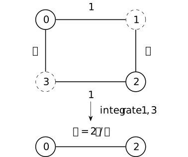
Solid circles are retained; dashed circles are integrated out. Orientations are suppressed because the quadratic energy is orientation independent. The bottom edge represents the induced coupling \(\beta \); its precision also has the diagonal term computed below.
The vectors \((1,1)^T/\sqrt 2\) and \((1,-1)^T/\sqrt 2\) diagonalize \(S\). Their eigenvalues are \[\begin {aligned} \sigma _+&=\alpha -\beta =\frac {s^2-(1+t)^2}{s}\\ &=\frac {a(a+2+2t)}{s},\\ \sigma _-&=\alpha +\beta =\frac {s^2-(1-t)^2}{s}\\ &=\frac {(a+2)(a+2t)}{s}. \end {aligned}\] Both are positive. The factorizations follow from \(s=1+t+a\); they also check positivity without appealing again to the general theorem. Put \[\mathcal D=a(a+2)(a+2t)(a+2+2t).\] Then \[\begin {aligned} \det C&=s^2,\qquad \det S=\mathcal D/s^2,\\ \det Q&=\det C\det S=\mathcal D,\\ c_C&=\frac {2\pi }{s},\qquad Z_S=\frac {2\pi s}{\sqrt {\mathcal D}},\\ Z_Q&=c_CZ_S=\frac {(2\pi )^2}{\sqrt {\mathcal D}}. \end {aligned}\] This reproduces the four-mode determinant and partition function. The effective action is \[\mathcal A_{\mathrm {eff}}(x)=\tfrac 12x^TSx+\log \frac {s}{2\pi }.\] Its constant records the integrated block.
A retained observable checks more than normalization. For \(F(x)=x_0x_2\), polynomial integrability and the marginal identity give \[\begin {aligned} \langle \phi _0\phi _2\rangle _Q &=\langle x_0x_2\rangle _S =(S^{-1})_{02}\\ &=\frac {\beta }{\alpha ^2-\beta ^2} =\frac {2ts}{\mathcal D}. \end {aligned}\] The indices \(0,2\) here name retained vertices. Inverting the displayed two-by-two matrix gives its off-diagonal entry \(\frac {\beta }{\det S}\), which proves the last equalities. Independently, the four-cycle spectral table gives \[\begin {aligned} 4\langle \phi _0\phi _2\rangle _Q &=\frac 1a-\frac 1{a+2}\\ &\quad -\frac 1{a+2t}+\frac 1{a+2+2t}\\ &=\frac {8ts}{\mathcal D}. \end {aligned}\] For the last equality, pair the first two terms and the last two: their difference has numerator \(2((a+2t)(a+2+2t)-a(a+2))=8ts\) over \(\mathcal D\). At \(t=m=1\), one obtains \[\begin {aligned} S&=\begin {pmatrix}7/3&-2/3\\-2/3&7/3\end {pmatrix},\\ S^{-1}&=\frac 1{15}\begin {pmatrix}7&2\\2&7\end {pmatrix},\\ \langle \phi _0\phi _2\rangle _Q&=\frac {2}{15},\\ c_C&=\frac {2\pi }{3},\quad Z_S=\frac {2\pi }{\sqrt 5},\quad Z_Q=\frac {4\pi ^2}{3\sqrt 5}. \end {aligned}\] Fixing the eliminated fields to zero instead gives precision \(A=3I_2\), covariance \(I_2/3\) and zero off-diagonal covariance. At \(t=2,m=1\), the same formulas give \[\begin {aligned} S&=\begin {pmatrix}11/4&-1\\-1&11/4\end {pmatrix},\\ \det S&=105/16,\\ S^{-1}&=\frac 1{105}\begin {pmatrix}44&16\\16&44\end {pmatrix}. \end {aligned}\] These are the parameters used in the symmetry comparison.
In the orthonormal sector coordinates \(x_\pm =(x_0\pm x_2)/\sqrt 2\) and \(y_\pm =(y_1\pm y_3)/\sqrt 2\), the couplings are \(-(1+t)\) and \(-(1-t)\). Their two eliminated pivots are both \(s\); each contributes \(\sqrt {2\pi/s}\), whose product is \(2\pi/s\). The factors \(1/\sqrt 2\) make these changes orthogonal, so there is no extra volume factor. The retained variance is \(\frac 12(\sigma _+^{-1}+\sigma _-^{-1})\), and the opposite covariance is \(\frac 12(\sigma _+^{-1}-\sigma _-^{-1})\). This agrees with the sector calculation.
There was no edge between vertices \(0\) and \(2\) in the supplied cycle. Elimination induces one in the effective quadratic form: \[S=\beta \begin {pmatrix}1&-1\\-1&1\end {pmatrix} +\sigma _+I_2.\] Thus \(\beta \) is an effective edge weight and \(\sigma _+\) an effective mass coefficient. This is a finite instance of fill-in: eliminating a single vertex joined to retained vertices with weights \(w_i\) and diagonal precision \(c>0\) subtracts \(ww^T/c\), creating off-diagonal entries \(-w_iw_j/c\) where no retained edge existed. The formula is the same Schur complement with \(H=-w\) and \(C=(c)\). Locality in the original graph need not survive elimination.
The half-turn preserves both sets \(R,U\) and swaps the two coordinates within each. For the swap matrix \(J\), the displayed \(S\) satisfies \(JSJ=S\); the induced two-site form retains this symmetry. The density and orthogonal-volume invariance then show that the retained law is invariant as well.
At \(m=0\), \(C=(1+t)I_2\) remains positive. Square completion and integration over the eliminated block still give \[S=\frac {2t}{1+t}\begin {pmatrix}1&-1\\-1&1\end {pmatrix}, \qquad c_C=\frac {2\pi }{1+t}.\] The retained constant mode has zero energy, so its full integral diverges by the kernel-box argument. The finite fiber factor cannot be divided by a finite retained partition function.
The global mean-zero law instead uses the space \(H=\{\phi :\sum _v\phi _v=0\}\) with its own induced volume. Its constraint \(x_0+x_2+y_1+y_3=0\) couples the two parts; \(H\) is neither their unrestricted product nor the product of their separate mean-zero lines. At \(t=1\), write a field in the three positive orthonormal modes as \(\phi =z_1u_1+z_2u_2+z_3u_3\). The coordinates are independent centered Gaussians of precisions \(2,2,4\). Put \[r=\frac {z_1+z_2}{\sqrt 2},\qquad v=\frac {z_1-z_2}{\sqrt 2}.\] This orthogonal change preserves \(z_1^2+z_2^2=r^2+v^2\) and two-dimensional volume. Thus \(r,v,z_3\) still have independent centered Gaussian laws of precisions \(2,2,4\). The retained unit coordinates satisfy \[\begin {aligned} x_-&=(\phi _0-\phi _2)/\sqrt 2=r,\\ x_+&=(\phi _0+\phi _2)/\sqrt 2=z_3/\sqrt 2. \end {aligned}\] Integrating the normalized \(v\) factor and changing variable \(z_3=\sqrt 2x_+\) give independent retained Gaussian densities of precisions \(2\) and \(8\). This density calculation identifies the law, not merely its covariance. Returning orthogonally to \((x_0,x_2)\) gives \[\begin {aligned} \operatorname {Cov}(x)&=\frac 1{16} \begin {pmatrix}5&-3\\-3&5\end {pmatrix},\\ Q_{H\to R}&=\begin {pmatrix}5&3\\3&5\end {pmatrix}. \end {aligned}\] These matrices multiply to the identity. The projected normalizer for this precision is \(\frac {2\pi }{\sqrt {16}}=\frac \pi 2\).
In contrast, directly setting \(m=0,t=1\) in the Schur formula gives the singular precision \(\begin {pmatrix}1&-1\\-1&1\end {pmatrix}\). Separately constraining that retained model to \(x_0+x_2=0\) leaves unit direction \((1,-1)/\sqrt 2\) with precision \(2\), normalizer \(\sqrt \pi \) and ambient covariance \(\frac 14\begin {pmatrix}1&-1\\-1&1\end {pmatrix}\). These are three distinct specified measures. The pinned affine law is another constraint with its own induced volume; fixing a vertex is not the marginal operation above.
The arithmetic pivot boundary is separate from the positive-real case. At \(m^2=1,t=-2\), \(s=t+2=0\), whereas \(\det Q=1\cdot 3\cdot (-3)\cdot (-1)=9\). Thus the full map can be invertible while this eliminated pivot is not. At \(t=-1\), the pivot exists but the later ratio denominator \(t+1\) vanishes. Neither value satisfies the positive-weight hypotheses used for the Gaussian laws here.
Proposition 9.6. Formal interaction under Gaussian elimination [fdip-0046]AGENTDRAFTED
- October 30, 2026
Proposition 9.6. Formal interaction under Gaussian elimination [fdip-0046]AGENTDRAFTED
- October 30, 2026
Eliminating a field with a quartic interaction generally creates quadratic and sextic terms. The coefficients through second order can be found by conditional Gaussian moments, while preserving a supplied symmetry and composition of eliminations.
Use the finite orthogonal sum \(E=X\mathbin \perp Y\), positive precision \(Q\), components \(A,B,C\), Schur precision \(S\) and scalar \(c_C\) of Gaussian elimination. Let \(T:E^4\to \mathbb R\) be a symmetric four-linear form and put \[V(u)=\frac {T(u,u,u,u)}{4!}.\] Write \(\mathcal P(X)\) for the polynomial function algebra. For \(x\in X\), let \(\eta \) have centered Gaussian law with covariance \(C^{-1}\) on \(Y\), and set \[v_x=(x,-C^{-1}B^\dagger x+\eta ).\] This is the conditional law of the eliminated field given the retained value. It is the conditional kernel with its two named summands exchanged; its covariance is \(C^{-1}\), whereas that proposition's retained-given-eliminated kernel has covariance \(A^{-1}\).
For a formal variable \(\lambda \), use ordinary power-series coefficients in \(\lambda \) and define the fiber effective interaction by \[\begin {aligned} F_\lambda (x)&=-\log \mathbb E_\eta e^{-\lambda V(v_x)},\\ \mathbb E_\eta e^{-\lambda V(v_x)} &=\sum _{n\geq 0}\frac {(-\lambda )^n}{n!} \mathbb E_\eta V(v_x)^n. \end {aligned}\] These are formal series in \(\lambda \) with coefficients in \(\mathcal P(X)\); the logarithm is the formal logarithm of a series with constant coefficient one. Every coefficient is finite by polynomial integrability. The notation \(O(\lambda ^3)\) means a series divisible by \(\lambda ^3\), not an analytic error estimate. With \[\begin {aligned} a(x)&=\mathbb E[V\mid x],\\ b(x)&=\mathbb E[V^2\mid x]-a(x)^2, \end {aligned}\] the first two coefficients are \[F_\lambda =\lambda a-\frac {\lambda ^2}{2}b+O(\lambda ^3).\] The degree-zero terms are retained: coefficientwise integration gives \[\begin {aligned} &\int _Y e^{-\frac 12\langle (x,y),Q(x,y)\rangle } e^{-\lambda V(x,y)}\,dy\\ &\qquad =c_Ce^{-\frac 12\langle x,Sx\rangle }e^{-F_\lambda (x)}. \end {aligned}\] Here \(dy\) is the specified Euclidean volume. This fiber logarithm integrates eliminated variables; it does not take the Legendre transform of a source-generating function used for a one-particle irreducible (1PI) effective action in [etingof2024mathematical, v2, Proposition 3.23, p. 50].
For a specified orthogonal flag \(E=X\mathbin \perp Y\mathbin \perp Z\), first eliminate \(Z\) and then \(Y\). All conditional expectations below use the original Gaussian law, with the \(Y\)-given-\(X\) kernel obtained after eliminating \(Z\). Put \[\begin {aligned} a_1(x,y)&=\mathbb E[V\mid x,y],\\ b_1(x,y)&=\mathbb E[V^2\mid x,y]-a_1(x,y)^2. \end {aligned}\] Both stages together give \[\begin {aligned} F_\lambda (x) ={}&\lambda \mathbb E[a_1\mid x]\\ &-\frac {\lambda ^2}{2}\bigl ( \mathbb E[b_1\mid x]+\operatorname {Var}(a_1\mid x)\bigr )\\ &+O(\lambda ^3), \end {aligned}\] which agrees with direct elimination of \(Y\oplus Z\). The first coefficient has degrees among \(4,2,0\); the second has degrees among \(6,4,2,0\). Particular components may vanish.
Proof.
- October 30, 2026
Proof.
- October 30, 2026
Expand the expectation as \(1-\lambda a+\lambda ^2\mathbb E[V^2\mid x]/2+O(\lambda ^3)\). The identity \(\log (1+u)=u-u^2/2+O(u^3)\) gives the displayed coefficient \(-b/2\). Square completion in Theorem 9.1 identifies the normalized conditional Gaussian and the raw scalar \(c_C\); applying it to each polynomial coefficient proves the fiber identity. No convergence or interchange of an infinite series and an integral is needed.
The first-stage interaction is \(F_1=\lambda a_1-\lambda ^2b_1/2+O(\lambda ^3)\). Hence \[e^{-F_1}=1-\lambda a_1+ \frac {\lambda ^2}{2}(a_1^2+b_1)+O(\lambda ^3).\] Take the \(Y\)-given-\(X\) expectation and the negative logarithm. This yields the stated two-stage formula. Polynomial integrability permits signed Fubini for every coefficient, so the tower identities for these Gaussian kernels give \[\begin {aligned} &\mathbb E[a_1\mid x]=\mathbb E[V\mid x],\\ &\mathbb E[b_1\mid x]+\operatorname {Var}(a_1\mid x)\\ &\qquad =\mathbb E[V^2\mid x]-\mathbb E[V\mid x]^2. \end {aligned}\] These identities also follow directly by expanding \(b_1\) and cancelling \(\mathbb E[a_1^2\mid x]\). They prove composition through the stated order without discarding any generated term.
The mean of \(v_x\) is linear in \(x\), and its centered noise is independent of \(x\). Expanding the four-linear tensor and pairing centered Gaussian factors by Wick's theorem leaves degrees \(4,2,0\) in \(a\). In \(\mathbb E[V^2\mid x]-\mathbb E[V\mid x]^2\), pairings with no contraction between the two copies of \(V\) cancel. Every remaining pairing uses at least two noise factors. The 8 original factors therefore leave at most 6 mean factors. An even number of noise factors is paired, giving only degrees \(6,4,2,0\). The homogeneous components are symmetric tensors on \(X\) by polarization; they need not be diagonal in a chosen coordinate basis.
Suppose a second such model is related by a linear isometric isomorphism \(L=L_X\oplus L_Y:E\to E'\) satisfying \(Q'L=LQ\) and \(V'\circ L=V\). Then \[F'_\lambda (L_Xx)=F_\lambda (x)\pmod {\lambda ^3}.\] Indeed the component identities give \(C'L_Y=L_YC\) and \((B')^\dagger L_X=L_YB^\dagger \). Thus \(L_Y\) transports the conditional mean and covariance, hence its Gaussian law and both moments \(a,b\). For two-stage elimination also require preservation of the supplied flag. In particular, a supplied finite group of these isometries preserves each induced coefficient. The result transports a given action; it does not select that action.
Wick contractions are [etingof2024mathematical, v2, Theorem 3.1 and Example 3.2, p. 29]. The perturbation convention in [etingof2024mathematical, v2, Section 3.3, p. 33] is \(B(u,u)/2-\sum _i g_iB_i(u,\ldots ,u)/i!\); here \(g_4=-\lambda \) and \(B_4=T\), at \(\hbar =1\). The conditional formulas and composition above are direct deductions using these contractions and the specified Gaussian kernels. The three-coordinate example exhibits every indicated degree.
Example 9.7. A quartic interaction and its retained four-point function [fdip-0047]AGENTDRAFTED
- October 30, 2026
Example 9.7. A quartic interaction and its retained four-point function [fdip-0047]AGENTDRAFTED
- October 30, 2026
On the real realization of \(\mathbb Q^3\), use coordinates \(x,y,z\), counting pairing \(g_0=I\) and the coordinate flag retaining \((x,y)\) and then \(x\). Fix the action \(q/2+\lambda V\), where \[\begin {aligned} q&=x^2+(y-x)^2+(z-y)^2,\\ V&=\frac {x^4+y^4+z^4}{4!},\\ Q&=\begin {pmatrix}2&-1&0\\-1&2&-1\\0&-1&1\end {pmatrix},\\ Q^{-1}&=\begin {pmatrix}1&1&1\\1&2&2\\1&2&3\end {pmatrix}. \end {aligned}\] The quadratic form is positive: the map \((x,y,z)\mapsto (x,y-x,z-y)\) is invertible. The fourth tensor of \(V\) has diagonal components one and all other components zero, with the displayed \(1/4!\) convention. Simultaneous sign reversal supplies an action of \(C_2\) preserving the pairing, action and flag.
For the fiber interaction after eliminating \(y,z\), the retained precision is \(S=1\), the scalar is \(c_C=2\pi \), and \[\begin {aligned} F_\lambda (x) ={}&\lambda \left (\frac {x^4}{8}+\frac {3x^2}{4}+\frac 58\right )\\ &-\lambda ^2\left (\frac {5x^6}{72}+\frac {53x^4}{48}\right .\\ &\hspace {38pt}\left .+\frac {97x^2}{24}+\frac {41}{24}\right ) +O(\lambda ^3). \end {aligned}\] In particular, a pure quartic interaction is not preserved by elimination. Adding a quadratic term and a constant still does not close this family: the second-order sextic coefficient is nonzero.
Proof.
- October 30, 2026
Proof.
- October 30, 2026
Under the Gaussian law conditional on \(x\), write \(y=x+\eta \) and \(z=x+\eta +\xi \), where \(\eta ,\xi \) are independent standard real Gaussians. This follows directly from \(q=x^2+\eta ^2+\xi ^2\) and the triangular change of variables of determinant one. Thus \[C^{-1}=\begin {pmatrix}1&1\\1&2\end {pmatrix}, \qquad S=1,\qquad c_C=2\pi .\] With \(a=\mathbb E[V\mid x]\) and \(b=\operatorname {Var}(V\mid x)\), use \(\mathbb E\eta ^{2k}=(2k-1)!!\), with \((-1)!!=1\), and zero odd moments. The first moments are \[\begin {aligned} \mathbb E[y^4\mid x]&=x^4+6x^2+3,\\ \mathbb E[z^4\mid x]&=x^4+12x^2+12. \end {aligned}\] For the second coefficient, the same pairings give \[\begin {aligned} \operatorname {Var}(y^4\mid x) &=16x^6+168x^4\\ &\quad +384x^2+96,\\ \operatorname {Var}(z^4\mid x) &=32x^6+672x^4\\ &\quad +3072x^2+1536,\\ \operatorname {Cov}(y^4,z^4\mid x) &=16x^6+216x^4\\ &\quad +600x^2+168. \end {aligned}\] For instance these mixed moments use \(\mathbb E\eta ^2=1\), \(\mathbb E(\eta +\xi )^2=2\) and \(\mathbb E[\eta (\eta +\xi )]=1\). The term \(x^4\) is constant at fixed \(x\), so \[\begin {aligned} a&=\frac {x^4}{8}+\frac {3x^2}{4}+\frac 58,\\ b&=\frac {5x^6}{36}+\frac {53x^4}{24} +\frac {97x^2}{12}+\frac {41}{12}. \end {aligned}\] Substitute these into \(F_\lambda =\lambda a-\lambda ^2b/2+O(\lambda ^3)\).
The same coefficients arise in two stages. First eliminate \(z=y+\xi \) with \(x,y\) fixed. The moments above, with \(x\) replaced by \(y\), give \[\begin {aligned} a_1(x,y)&=\frac {x^4+2y^4+6y^2+3}{24},\\ b_1(x,y)&=\frac {y^6}{36}+\frac {7y^4}{24} +\frac {2y^2}{3}+\frac 16. \end {aligned}\] Here \(a_1=\mathbb E[V\mid x,y]\) and \(b_1=\operatorname {Var}(V\mid x,y)\); the terms \(x^4,y^4\) are constant at this stage. Next take \(y=x+\eta \). The even moments \(1,3,15,105\) of orders \(2,4,6,8\) give \[\begin {aligned} \mathbb E[a_1\mid x]&=\frac {x^4}{8}+\frac {3x^2}{4}+\frac 58=a,\\ \mathbb E[b_1\mid x]&=\frac {x^6}{36}+\frac {17x^4}{24} +\frac {11x^2}{3}+\frac {17}{8},\\ \operatorname {Var}(a_1\mid x)&=\frac {x^6}{9}+\frac {3x^4}{2} +\frac {53x^2}{12}+\frac {31}{24}. \end {aligned}\] The last two lines sum to \(b\). Thus the two-stage identity reproduces both direct coefficients, including their constants.
A source on a retained space \(X\) is a linear functional \(j\in X^*\), coupled by multiplying the weight by \(e^{j(x)}\). Under a retained linear isomorphism \(L_X:X\to X'\), a source \(j'\in (X')^*\) pulls back to \(j'\circ L_X\), since \(e^{j'(L_Xx)}=e^{(j'\circ L_X)(x)}\). In this example \(X=\mathbb R\) and \(j(x)=Jx\), with \(J\) treated as a formal scalar variable. Let \(\mu _Q\) be the normalized Gaussian law. Define \[\begin {aligned} W(J,\lambda ) ={}&\log \mathbb E_{\mu _Q}e^{Jx-\lambda V}\\ &-\log \mathbb E_{\mu _Q}e^{-\lambda V}. \end {aligned}\] Each coefficient in the two formal variables \(J,\lambda \) is a finite Gaussian moment. Thus \(W(0,\lambda )=0\). Coefficients use ordinary powers of \(\lambda \); 4 source derivatives multiply the coefficient of \(J^4\) by \(4!\). The connected four-point function in this scalar example is \[\begin {aligned} G_c^{(4)}(\lambda ) &=\left .\frac {\partial ^4W}{\partial J^4}\right |_{J=0}\\ &=-3\lambda +101\lambda ^2+O(\lambda ^3). \end {aligned}\]
Proof.
- October 30, 2026
Proof.
- October 30, 2026
Write \[\mathbb E_\lambda [P]= \frac {\mathbb E_{\mu _Q}[P e^{-\lambda V}]} {\mathbb E_{\mu _Q}e^{-\lambda V}}\] as a formal ratio. After eliminating \(y,z\), both numerator and denominator are expectations for \(x\sim N(0,1)\) with weight \[\begin {aligned} e^{-F_\lambda (x)}={}&1-\lambda a(x)\\ &+\frac {\lambda ^2}{2}(a(x)^2+b(x))\\ &+O(\lambda ^3). \end {aligned}\] The scalar \(c_C\) cancels from this ratio, but the constant terms in \(a,b\) are included before the division. Gaussian moments give \[\begin {aligned} \mathbb E[e^{-F_\lambda }]&= 1-\frac 74\lambda +\frac {1351}{96}\lambda ^2+O(\lambda ^3),\\ \mathbb E[x^2e^{-F_\lambda }]&= 1-\frac {19}{4}\lambda +\frac {1981}{32}\lambda ^2+O(\lambda ^3),\\ \mathbb E[x^4e^{-F_\lambda }]&= 3-\frac {105}{4}\lambda +\frac {14799}{32}\lambda ^2\\ &\qquad +O(\lambda ^3). \end {aligned}\] Dividing yields \[\begin {aligned} \mathbb E_\lambda [x^2]&= 1-3\lambda +\frac {511}{12}\lambda ^2+O(\lambda ^3),\\ \mathbb E_\lambda [x^4]&= 3-21\lambda +\frac {767}{2}\lambda ^2+O(\lambda ^3). \end {aligned}\] Sign reversal makes the odd moments zero and \(W(-J,\lambda )=W(J,\lambda )\). Expanding the logarithm in \(J\) therefore gives \[G_c^{(4)}=\mathbb E_\lambda [x^4] -3\bigl (\mathbb E_\lambda [x^2]\bigr )^2,\] which is the asserted coefficient.
These are formal expansions. For real \(\lambda \geq 0\), the original interaction is nonnegative, so its exact partition integral is positive and bounded by the Gaussian normalizer. Polynomial moments remain finite. A real source also gives a finite integral, since the linear tilt of a positive Gaussian is integrable. None of this asserts convergence of the formal series at zero. For every fixed \(\lambda >0\), exponentiating only the displayed second-order \(F_\lambda \) instead gives a nonintegrable retained weight: its leading term is \(-5\lambda ^2x^6/72\), so \(e^{-x^2/2-F_\lambda ^{(2)}(x)}\) grows at infinity. Here \(F_\lambda ^{(2)}\) denotes the displayed polynomial through \(\lambda ^2\).
The Gaussian moment rule is [etingof2024mathematical, v2, Theorem 3.1, p. 29]. The connected-logarithm interpretation is [etingof2024mathematical, v2, Theorem 3.11, p. 38], with \(g_4=-\lambda \) and the zero-source logarithm subtracted. The rational coefficients above are the explicit calculation for this supplied model. Stationary elimination retains its sextic term but omits the fluctuation-generated lower degrees.
Remark 9.8. Stationary elimination and the tree contribution [fdip-0048]AGENTDRAFTED
- October 30, 2026
Remark 9.8. Stationary elimination and the tree contribution [fdip-0048]AGENTDRAFTED
- October 30, 2026
For the three-coordinate quartic action, formal power-series stationarity around the Gaussian stationary point and integration of the eliminated fluctuations agree on some coefficients but not all. Write \(u=(y,z)\), \(u_0=(x,x)\) and \[H=C^{-1}=\begin {pmatrix}1&1\\1&2\end {pmatrix}.\] At fixed \(x\), the action is \[\begin {aligned} \mathcal A(x,u)={}&\frac {x^2}{2} +\frac 12(u-u_0)^TC(u-u_0)\\ &+\lambda V(x,u). \end {aligned}\] There is a unique formal stationary solution \(u_*(x,\lambda )=u_0+O(\lambda )\). Its stationary value is \[\begin {aligned} \mathcal A_{\mathrm {cl}}(x,\lambda ) &=\mathcal A(x,u_*(x,\lambda ))\\ &=\frac {x^2}{2}+\frac {\lambda x^4}{8} -\frac {5\lambda ^2x^6}{72}+O(\lambda ^3). \end {aligned}\] For real \(\lambda \geq 0\), the action is coercive and strictly convex in \(u\): the quadratic Hessian \(C\) is positive definite and the quartic summands are convex. It therefore has a unique minimizer. The calculation below uses only formal power-series stationarity around \(u_0\) at \(\lambda =0\).
Proof.
- October 30, 2026
Proof.
- October 30, 2026
The equation is \(C(u-u_0)+\lambda \nabla _uV(x,u)=0\). Since \(C\) is invertible, comparison of successive powers of \(\lambda \) uniquely determines the formal coefficients. Put \[r=\nabla _uV(x,u_0)=\frac {x^3}{6}\binom {1}{1}.\] The first coefficient gives \(u_*=u_0-\lambda Hr+O(\lambda ^2)\). Substitution in the action yields \[\mathcal A_{\mathrm {cl}}= \frac {x^2}{2}+\lambda V(x,u_0) -\frac {\lambda ^2}{2}r^THr+O(\lambda ^3).\] Now \(V(x,u_0)=x^4/8\) and \(r^THr=5x^6/36\). This proves the stationary coefficient without replacing a Gaussian integral by a minimum.
To distinguish fluctuation terms, take \(\hbar >0\), let \(\eta _\hbar \) be centered Gaussian with covariance \(\hbar H\), and use the normalized fiber expression \[\begin {aligned} &F_{\lambda ,\hbar }(x)\\ &\quad =-\hbar \log \mathbb E\exp \left ( -\frac {\lambda }{\hbar }V(x,u_0+\eta _\hbar )\right ). \end {aligned}\] Expand formally in \(\lambda \); through the second order its coefficients are polynomials in \(\hbar \): \[\begin {aligned} F_{\lambda ,\hbar }(x) ={}&\lambda \left (\frac {x^4}{8}+\frac {3\hbar x^2}{4} +\frac {5\hbar ^2}{8}\right )\\ &-\lambda ^2\left (\frac {5x^6}{72} +\frac {53\hbar x^4}{48}\right .\\ &\hspace {38pt}\left .+\frac {97\hbar ^2x^2}{24} +\frac {41\hbar ^3}{24}\right )\\ &+O(\lambda ^3). \end {aligned}\] Indeed each Gaussian pairing contributes one \(\hbar \); the first coefficient is \(\mathbb E V\) and the second is \(-\operatorname {Var}(V)/(2\hbar )\). Applying this scaling to the explicit moment calculation proves the formula.
Consequently, through order \(\lambda ^2\), the coefficient of \(\hbar ^0\) in this fiber interaction is \[\begin {aligned} [\hbar ^0]F_{\lambda ,\hbar }(x) &=\frac {\lambda x^4}{8}-\frac {5\lambda ^2x^6}{72} +O(\lambda ^3)\\ &=\mathcal A_{\mathrm {cl}}(x,\lambda )-\frac {x^2}{2} +O(\lambda ^3). \end {aligned}\] The retained Gaussian action \(x^2/2\) must be added to recover the full stationary value. At \(\lambda =0\) the normalized fiber interaction is zero, whereas that stationary value is \(x^2/2\).
This is the tree contribution in the loop grading of [etingof2024mathematical, v2, Section 3.6 and Theorem 3.12, pp. 38-39]. We adapt Etingof's rescaled convention to the displayed weight \(\exp (-\lambda V/\hbar )\) with covariance \(\hbar H\): a Gaussian contraction contributes \(\hbar \) and an interaction vertex contributes \(\hbar ^{-1}\). The logarithm selects connected graphs; after multiplication by \(-\hbar \), a connected graph with \(e\) contracted edges and \(v\) interaction vertices has power \(\hbar ^{e-v+1}\). Its number of independent cycles is \(e-v+1\); zero cycles means a tree. Thus connected contractions need not be trees. In the displayed second-order coefficient, only the sextic term is at tree order; its quartic, quadratic and constant companions have positive powers of \(\hbar \). The source's stationary-action convention is applied to the shifted fiber action, whose unperturbed minimum is zero, which explains the subtraction of \(x^2/2\).
The retained law still refers to chosen field coordinates and a chosen split. Which changes merely relabel and transport this model, and which change its predictions?
10. Backgrounds and symmetry [fdip-0019]AGENTDRAFTED
- October 20, 2026
10. Backgrounds and symmetry [fdip-0019]AGENTDRAFTED
- October 20, 2026
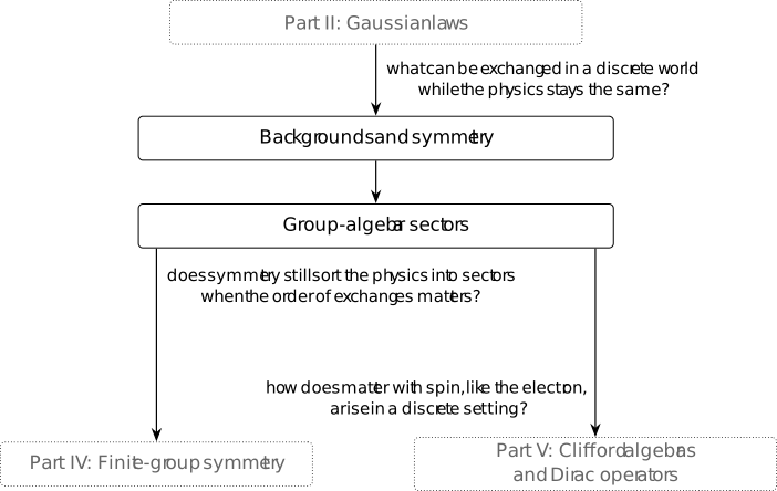
Which changes preserve the model while transporting its equations, expectations and retained law? A symmetry preserves the specified data; it transports observables rather than fixing every observable function individually. Relabellings of a finite carrier are discrete permutations, although finite-dimensional field fibres can also admit continuous internal actions. Here endpoint transport, coherent edge reversals and preserved weights control incidence and operator transport; the half-turn of the alternating cycle gives a concrete action. With compatible perfect pairings and transport of the chosen retained split, the observable functionals and marginal transport as well. The duality, split-map and normalized-functional conventions are assumed.
A finite background records the supplied data. The Gaussian integral and marginal theorem identify transported functionals with normalized laws. Fixed labels, broken weights and nonstable partitions give different failures. The trace ratio distinguishes weighted cycles even under a broader comparison allowing positive scaling. These examples prepare enriched-background comparisons, where the permitted arrows must specify exactly what survives.
Definition 10.1. Signed arrows preserve endpoints before incidence [fdip-003B]AGENTDRAFTED
- October 29, 2026
Definition 10.1. Signed arrows preserve endpoints before incidence [fdip-003B]AGENTDRAFTED
- October 29, 2026
Reversing an oriented edge changes the sign of its difference, but does not erase its endpoints. Fix a commutative unital ring \(k\) and two finite incidence presentations \((V,E,s,h)\) and \((V',E',s',h')\). Equip them with weights \(w:E\to k\), \(w':E'\to k\), scalars \(\mu ,\mu '\in k\), and retained subsets \(R\subseteq V\), \(R'\subseteq V'\). Empty carriers, loops and distinct parallel edge labels are allowed.
Write \(C_2=\{+,-\}\) for the abstract group with \(-\cdot -=+\), and \(\sigma :C_2\to k^\times \) for \(\sigma (+)=1\), \(\sigma (-)=-1\). A signed endpoint arrow consists of bijections \(p:V\to V'\), \(q:E\to E'\) and signs \(\varepsilon :E\to C_2\) such that \[\begin {aligned} \varepsilon (e)=+&:\quad s'q(e)=ps(e),\quad h'q(e)=ph(e),\\ \varepsilon (e)=-&:\quad s'q(e)=ph(e),\quad h'q(e)=ps(e),\\ w'q&=w,\qquad \mu '=\mu ,\qquad pR=R'. \end {aligned}\] The signs are abstract orientation data, even when \(1=-1\) in \(k\). An arrow with all signs \(+\) is directed. For the real Gaussian backgrounds, directed arrows are their exact relabelings, with \(\mu =m^2\); positivity of mass then recovers \(m'=m\).
Composition applies the right arrow first. The composite with \((p',q',\varepsilon ')\) is \[\bigl (p'p,q'q,\ e\mapsto \varepsilon '(q(e))\varepsilon (e)\bigr ).\] Identity arrows have identity bijections and all signs \(+\). The inverse of \((p,q,\varepsilon )\) has bijections \(p^{-1},q^{-1}\) and the sign \(\varepsilon (e)\) at \(q(e)\). These operations make the declared objects and arrows a groupoid: composition is associative, identities exist, and every arrow is invertible, as for an action groupoid.
Proof.
- October 29, 2026
Proof.
- October 29, 2026
For two arrows, zero, one or two endpoint exchanges occur according as their signs are \((+,+)\), \((+,-)\) or \((-,+)\), and \((-,-)\). These give, respectively, the product signs \(+,-,+\). Thus composition has the required endpoints. Also \(w''q'q=w'q=w\) and \(p'pR=p'R'=R''\); the scalar stays fixed. The inverse applies the same sign twice, so restores endpoints and gives sign \(+\). For three arrows either parenthesization gives the sign \[\varepsilon ''(q'q(e))\varepsilon '(q(e))\varepsilon (e).\] Associativity in \(C_2\) and of the bijections proves associativity; the stated identities and inverses satisfy both unit and inverse laws.
Let \(M=k^V\), \(N=k^E\) and similarly \(M',N'\), with incidence maps \((df)(e)=f(h(e))-f(s(e))\). The induced ordinary linear maps are \[\begin {aligned} (Pf)(p(v))&=f(v),&P&:M\to M',\\ (Ja)(q(e))&=\sigma (\varepsilon (e))a(e),&J&:N\to N'. \end {aligned}\] They are isomorphisms: \(P^{-1}f'=f'\circ p\) and \((J^{-1}a')(e)=\sigma (\varepsilon (e))a'(q(e))\). Evaluation at \(q(e)\), in the two endpoint cases, gives \[d'P=Jd:M\longrightarrow N'.\] Both differences vanish on a loop; the endpoint condition still remembers where that loop is attached.
For a left action of a group \(\Gamma \), take actions \(p_g,q_g\) on the vertex and edge sets. A signed endpoint action additionally requires \[\varepsilon _1(e)=+,\qquad \varepsilon _{gk}(e)=\varepsilon _g(q_k(e))\varepsilon _k(e).\] Thus the arrow assigned to \(gk\) is the composite of those assigned to \(g\) and \(k\). The induced maps satisfy \(P_gP_k=P_{gk}\) and \(J_gJ_k=J_{gk}\). Indeed evaluation at \(p_{gk}(v)\) gives \(f(v)\) on both sides of the first equation; at \(q_{gk}(e)\) the second has coefficient \(\sigma (\varepsilon _g(q_k(e)))\sigma (\varepsilon _k(e))a(e)\). Identity signs and maps give the identity operators. These are linear representations on two distinct carriers; no faithfulness is assumed.
A weaker signed-incidence symmetry requires the same actions, abstract sign cocycle and weight preservation, but only the incidence equation \(dP_g=J_gd\), instead of the endpoint equations. It is an incidence intertwiner and suffices for operator transport. It need not be a graph automorphism; loops and characteristic two distinguish the requirements. The concrete half-turn satisfies the stronger endpoint conditions.
The left-action and equivariance conventions are [milne2025group, Definition 4.1, pp. 57-58]. [milne2025group, Example 7.1(b), p. 101] gives a permutation representation over a field; the ring and signed endpoint construction above is proved directly. The incidence convention in [spielman2009effective, Section 2.1, pp. 4-5] concerns a connected undirected positive-weight graph with a chosen orientation; the endpoint-difference definition here also allows loops, parallel labels and arbitrary coefficients.
Mathlib's Representation.ofMulAction sends the free
basis vector at \(v\) to that at \(g\cdot v\).
Finsupp.linearEquivFunOnFinite identifies its coefficients
with functions on a finite set, yielding inverse precomposition for a
group action. Representation.IntertwiningMap bundles an
intertwiner between already supplied representations. Neither supplies
the endpoint equations or abstract sign cocycle above.
Example 10.2. What zero incidence and scalar signs forget [fdip-003C]AGENTDRAFTED
- October 29, 2026
Example 10.2. What zero incidence and scalar signs forget [fdip-003C]AGENTDRAFTED
- October 29, 2026
The signed endpoint equations retain information that an incidence operator alone can lose. Take vertices \(\{0,1\}\) and one loop \(e\) attached at \(0\). Its incidence map is zero over every ring. Swapping the vertices, fixing \(e\) and choosing sign \(+\) therefore intertwines incidence and preserves any weight on \(e\). Nevertheless \(s(q(e))=0\ne 1=p(s(e))\); the same obstruction holds for sign \(-\), since both endpoints of the loop are \(0\). This is a signed-incidence symmetry, but not a signed endpoint arrow.
A separate loss concerns composition. Let \(C_3=\{1,g,g^2\}\) fix a single loop and its vertex. Assign abstract signs \(\varepsilon _1=+\), \(\varepsilon _g=\varepsilon _{g^2}=-\). Every endpoint and zero-incidence equation holds separately. But the action cocycle at \(g\cdot g=g^2\) would require \[\varepsilon _{g^2}=\varepsilon _g\varepsilon _g=+,\] contrary to the assigned \(-\). Thus these arrows do not define a \(C_3\)-action. Over a ring of characteristic two the scalar maps all become the identity because \(-1=1\); even their representation equations then conceal the failed abstract cocycle. Orientation data remain subject to the abstract \(C_2\) law.
By contrast, one edge \(e:0\to 1\) admits the vertex swap with fixed edge label and sign \(-\). Its endpoints reverse as required, and using this arrow twice gives sign \(+\) and identity bijections. For fields, \[(dPf)(e)=f(0)-f(1)=-(df)(e)=(Jdf)(e).\] It is a valid signed symmetry. Parallel labels are still distinct: an edge bijection may permute them, but never identifies two labels. Each sign must satisfy its own endpoint rule and the composition law.
These calculations use the endpoint-difference construction of Definition 10.1.
[spielman2009effective, Section 2.1, pp. 4-5] allows an arbitrary orientation of each edge. The calculations explain its extension in the signed endpoint construction.
[milne2025group, Definition 4.1, p. 57] gives the group-law requirement. Neither source is being asserted to contain these loop or characteristic-two examples.
Example 10.3. The half-turn on vertex and edge fields [fdip-000J]AGENTDRAFTED
- October 17, 2026
Example 10.3. The half-turn on vertex and edge fields [fdip-000J]AGENTDRAFTED
- October 17, 2026
The alternating four-cycle has a symmetry for every \(t>0\), including unequal weights. Let \(C_2=\{1,r\}\) with \(r^2=1\). Its left actions on the distinct vertex and edge sets \(V=\mathbb Z/4\mathbb Z\) and \(E=\{e_0,e_1,e_2,e_3\}\) are \[r\cdot i=i+2,\qquad r\cdot e_i=e_{i+2}.\] Indices are modulo \(4\). These permutations square to the identity, preserve the endpoints \(e_i:i\to i+1\), and preserve the weights \((1,t,1,t)\). Milne's [milne2025group, Definition 4.1, p. 57] gives the left-action convention; his [milne2025group, Example 7.1(b), p. 101] constructs the associated permutation representation.
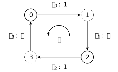
The half-turn exchanges \(0,2\) and \(1,3\), and exchanges \(e_0,e_2\) and \(e_1,e_3\). Directed arrows and their weights agree after rotation. Solid vertices form the retained set \(\{0,2\}\); the dashed vertices form its complement. Each set is preserved.
The induced maps on real fields use inverse precomposition: \[\begin {aligned} P:\mathbb R^V&\to \mathbb R^V,&(P\phi )_i&=\phi _{i-2},\\ U:\mathbb R^E&\to \mathbb R^E,&(Ua)(e_i)&=a(e_{i-2}). \end {aligned}\] Both maps have the coordinate array \[\begin {pmatrix} 0&0&1&0\\0&0&0&1\\1&0&0&0\\0&1&0&0 \end {pmatrix},\] but their domains differ. They satisfy \(P^2=I\) and \(U^2=I\). Sending \(1\) to the identity and \(r\) to these maps gives two real linear representations of \(C_2\).
Write \(\delta _i(j)=\mathbf 1_{j=i}\) for the vertex coordinate basis and \(\eta _i(e_j)=\mathbf 1_{j=i}\) for the edge coordinate basis. Then \(P\delta _0=\delta _2\ne \delta _0\) and \(U\eta _0=\eta _2\ne \eta _0\). Since \(r\) is the only nonidentity element of \(C_2\), both representations are faithful. Finite coordinate reindexing preserves the counting pairings; weight preservation gives \[\begin {aligned} P^TP&=I,\qquad U^TU=I,\\ U^TWU&=W, \end {aligned}\] where \(W=\operatorname {diag}(1,t,1,t)\). The last identity also preserves the weighted edge pairing.
The two representations interact through the incidence matrix. With its edge-by-vertex convention from [spielman2009effective, Section 2.1, p. 4], \[\begin {aligned} (BP\phi )(e_i)&=\phi _{i+1-2}-\phi _{i-2}\\ &=(UB\phi )(e_i). \end {aligned}\] Thus \(BP=UB\): the incidence map is equivariant between the vertex and edge actions.
The same formulas define linear representations over any nonzero commutative unital ring, with any period-two weights in that ring. The delta witnesses still prove faithfulness because \(1\ne 0\). Over the zero ring the two field modules have one element, so this faithfulness assertion is excluded. The positive real weights above are the specialization used for Gaussian laws.
This is the all-positive case of a signed endpoint action. The general endpoint composition, abstract orientation cocycle and weaker signed-incidence symmetry have that defining address. The loop and reversal examples explain why endpoint and sign coherence cannot be inferred from the incidence intertwiner alone.
Mathlib's Representation.ofMulAction sends a coordinate
basis vector at \(v\) to the one at \(g\cdot v\). Its finitely supported
coefficient module is identified with all functions on a finite set by
Finsupp.linearEquivFunOnFinite, giving the inverse-precomposition
convention above. Representation.IntertwiningMap bundles
a linear map with the equation \(B P_g=U_gB\). These interfaces do not
provide the particular incidence identity or the coherent signed-edge
action without their proofs.
Theorem 10.4. Pairing isometries transport incidence operators [fdip-003D]AGENTDRAFTED
- October 29, 2026
Theorem 10.4. Pairing isometries transport incidence operators [fdip-003D]AGENTDRAFTED
- October 29, 2026
Let \(k\) be a commutative unital ring. Give \(M,N,M',N'\) chosen perfect symmetric pairings, and let \(d:M\to N\), \(d':M'\to N'\) be ordinary linear maps. Suppose the linear isomorphisms \(P:M\to M'\), \(J:N\to N'\) preserve these pairings and satisfy \(d'P=Jd\). Let \(W:N\to N\), \(W':N'\to N'\) be self-adjoint maps with \(W'J=JW\). For a fixed \(\mu \in k\), put \[L=d^\dagger Wd,\qquad Q=L+\mu I_M,\] and define \(L',Q'\) by the primed data. Then \[\begin {aligned} (d')^\dagger &=Pd^\dagger J^{-1}:N'\to M',\\ L'&=PLP^{-1},\qquad Q'=PQP^{-1}. \end {aligned}\] If \(Q\) is an isomorphism, so is \(Q'\), and its inverse response satisfies \[G'=(Q')^{-1}=PQ^{-1}P^{-1}=PGP^{-1}.\] Consequently \(Qf=j\) implies \(Q'(Pf)=Pj\).
Proof.
- October 29, 2026
Proof.
- October 29, 2026
For \(z'\in M'\), pairing preservation gives \(b_{M'}(Px,z')=b_M(x,P^{-1}z')\). The uniqueness of the adjoint therefore gives \(P^\dagger =P^{-1}\), and similarly \(J^\dagger =J^{-1}\). From \(d'=JdP^{-1}\), the adjoint product law gives \((d')^\dagger =Pd^\dagger J^{-1}\). Thus \[\begin {aligned} L'&=Pd^\dagger J^{-1}W'JdP^{-1}\\ &=Pd^\dagger WdP^{-1}=PLP^{-1}. \end {aligned}\] Here \(J^{-1}W'J:N\to N\) equals \(W\); every composition is typed. The same scalar \(\mu \) gives the assertion for \(Q\). Multiplication in either order proves that \(PQ^{-1}P^{-1}\) is the inverse of \(Q'\). Finally \(Q'Pf=PQf=Pj\).
For signed endpoint arrows, the finite function modules have perfect counting duality, including empty carriers. Reindexing gives \[\begin {aligned} b_{M'}(Pf,Pg)&=\sum _{v\in V}f(v)g(v),\\ b_{N'}(Ja,Jb)&=\sum _{e\in E}\sigma (\varepsilon (e))^2a(e)b(e) =b_N(a,b). \end {aligned}\] Multiplication by transported weights obeys \(W'J=JW\), by evaluation at \(q(e)\). Thus the theorem applies without inverting any weight. It also applies to the weaker signed-incidence symmetries. The weighted edge pairing is \(b_W(a,b)=b_N(a,Wb)\); its adjoint of \(d\) into the counting vertex pairing is \(d^\dagger W\), whereas \(d^\dagger \) uses the counting edge pairing. The expression \(d^\dagger Wd\) does not require \(b_W\) to be perfect.
The inverse hypothesis cannot be replaced by a unit mass scalar. Over \(\mathbb Z\), a unit-weight edge on two vertices with \(\mu =1\) has \(Q=\begin {pmatrix}2&-1\\-1&2\end {pmatrix}\). Solving \(Q(x,y)=(1,0)\) would require \(x=2y\) and \(3y=1\), which is impossible in \(\mathbb Z\). This \(Q\) is not even surjective.
For automorphisms the conjugacies are commutation identities. They concern symmetric bilinear pairings over fixed coefficients. A grading is preserved only if \(P\) preserves its graded pieces; a star is preserved only if \(P\) commutes with that star. A nontrivial coefficient involution and Hermitian adjoint need their own conventions.
The proof uses the chosen duality construction in Proposition 3.3,
with the Hom convention of
[stacks2017stacks, Section 10.10], Tag 0581.
For real graph incidence, the energy convention is
[spielman2009effective, Section 2.1, pp. 4-5]; the displayed
ring transport is a direct deduction, not a positivity theorem.
Mathlib's Matrix.reindexLinearEquiv and
Matrix.reindexRingEquiv support its coordinate reindexing
specialization, without supplying the endpoint or pairing hypotheses.
Proposition 10.5. Transport of the retained Schur map [fdip-003E]AGENTDRAFTED
- October 29, 2026
Proposition 10.5. Transport of the retained Schur map [fdip-003E]AGENTDRAFTED
- October 29, 2026
Over a commutative unital ring \(k\), give \(M=X\oplus Y\) and \(M'=X'\oplus Y'\) chosen splittings. Suppose isomorphisms \(P:M\to M'\), \(P_X:X\to X'\), \(P_Y:Y\to Y'\) preserve the inclusions and projections: \[\begin {aligned} P\iota _X&=\iota '_XP_X,&P\iota _Y&=\iota '_YP_Y,\\ \pi '_XP&=P_X\pi _X,&\pi '_YP&=P_Y\pi _Y. \end {aligned}\] Let \(Q'=PQP^{-1}\). Write its 4 split components and those of \(Q\) as \(A:X\to X\), \(B:Y\to X\), \(E:X\to Y\), \(C:Y\to Y\), and their primed versions. Then \[\begin {aligned} A'&=P_XAP_X^{-1},&B'&=P_XBP_Y^{-1},\\ E'&=P_YEP_X^{-1},&C'&=P_YCP_Y^{-1}. \end {aligned}\] If \(C\) is invertible, the split Schur maps obey \[S'=P_XSP_X^{-1},\qquad S=A-BC^{-1}E.\] For \(K=C^{-1}E:X\to Y\), \(K'=(C')^{-1}E'\), \[K'P_X=P_YK,\qquad -K'(P_Xx)=P_Y(-Kx).\] Thus the eliminated-equation field \(y_*(x)=-Kx\), the unique solution of the lower equation with zero source, is transported with its sign intact.
Proof.
- October 29, 2026
Proof.
- October 29, 2026
For indices \(i,j\in \{X,Y\}\), the inclusion and projection identities give \[\pi '_iQ'\iota '_j =P_i(\pi _iQ\iota _j)P_j^{-1}.\] Taking \((i,j)=(X,X),(X,Y),(Y,X),(Y,Y)\) gives all 4 typed identities. Inverting the last one gives \((C')^{-1}=P_YC^{-1}P_Y^{-1}\). Substitution cancels each adjacent \(P_Y^{-1}P_Y\) in \(B'(C')^{-1}E'\), proving the Schur formula. The same substitution in \(K'\) proves \(K'P_X=P_YK\) and hence the transport identity for this field.
When \(Q\) is also invertible, the inverse-compression theorem says \[S^{-1}=\pi _XQ^{-1}\iota _X.\] Conjugating and using the split maps gives \[(S')^{-1}=P_XS^{-1}P_X^{-1} =\pi '_X(Q')^{-1}\iota '_X.\] This uses an actual inverse. No pairing has been assumed; only for an orthogonal split and self-adjoint \(Q\) does one further have \(E=B^\dagger \), by Proposition 4.5. For an orthogonal split of finite-dimensional real inner-product spaces and a positive self-adjoint \(Q\), this field is also stationary for the quadratic action in the eliminated variable, by the real square-completion argument.
For a vertex bijection \(p:V\to V'\), let \(R'=pR\), \(X=k^R\), \(X'=k^{R'}\), and let \(P_R\) be inverse precomposition by \(p|_R\). At \(p(v)\), \(v\in R\), both sides of \[\pi _{R'}P=P_R\pi _R\] take the value \(f(v)\). The target space is \(k^{pR}\), even if the labels of \(R\) and \(pR\) differ. This equation supplies the moving projection square in Gaussian marginal transport.
If a group action preserves \(R\), its restrictions compose on \(k^R\) and the square becomes \(\pi _RP_g=P_{g,R}\pi _R\). Faithfulness of the full action need not survive restriction: a permutation moving only eliminated vertices acts trivially on retained fields. The opposite-pair half-turn has a separate nontrivial retained action.
Stable subsets and equivariance follow the convention of [milne2025group, p. 58]. The real Schur convention is [boyd2004convex, Appendix A.5.5, pp. 650-651], with the source's first pivot exchanged to the eliminated \(C\) block. The typed transport proof above uses only the chosen splitting, and does not by itself supply any integral or Gaussian normalizer.
Proposition 10.6. Transport of polynomial observables and functionals [fdip-003F]AGENTDRAFTED
- October 29, 2026
Proposition 10.6. Transport of polynomial observables and functionals [fdip-003F]AGENTDRAFTED
- October 29, 2026
Let \(k\) be a commutative unital ring. For a \(k\)-module \(M\), write \(\mathcal P_k(M)\) for the unital \(k\)-subalgebra of functions \(M\to k\) generated by ordinary linear functionals. This extends the intrinsic real polynomial functions using the same pointwise operations. These are actual functions: over finite fields, distinct formal polynomials can have identical evaluations.
For a linear isomorphism \(P:M\to M'\), pullback gives a unital algebra isomorphism \[P^*:\mathcal P_k(M')\longrightarrow \mathcal P_k(M),\qquad P^*F'=F'\circ P.\] An already supplied normalized functional \(\omega \) on \(\mathcal P_k(M)\) transports to \(\omega '=\omega \circ P^*\). For the moving split square, the retained functionals \(\omega _X=\omega \circ \pi ^*\) and \(\omega '_{X'}=\omega '\circ (\pi ')^*\) satisfy \[\omega '_{X'}=\omega _X\circ P_X^*.\] Here \(\pi :M\to X\), \(\pi ':M'\to X'\) are the specified projections, and \(\pi 'P=P_X\pi \).
Proof.
- October 29, 2026
Proof.
- October 29, 2026
Precomposition preserves sums, scalar multiples, products and the constant function \(1\), by evaluation. A linear functional on \(M'\) composed with \(P\) is linear on \(M\), so pullback preserves the generated polynomial algebras. Its inverse is \((P^{-1})^*\). For composable maps, \((P'P)^*F''=F''\circ P'\circ P=P^*((P')^*F'')\); identity pullback is identity. This proves contravariance as well.
Linearity of \(\omega '\) and \(\omega '(1)=\omega (1)=1\) follow directly, or by algebra-map pullback. The section \(\iota _X\) of \(\pi \) makes \(\pi ^*\) injective: \(f\circ \pi =g\circ \pi \) implies \(f=g\) after composition with \(\iota _X\). Thus \(\omega _X\) is restriction to the image of \(\pi ^*\), identified with \(\mathcal P_k(X)\). Finally, for each \(f'\in \mathcal P_k(X')\) and \(x\in M\), \[\begin {aligned} P^*(\pi ')^*f'(x) &=f'(\pi 'Px)\\ &=f'(P_X\pi x)=(\pi ^*P_X^*f')(x). \end {aligned}\] Applying \(\omega \) gives the asserted retained-functional equality.
Over \(\mathbb R\) with the identity involution, or over \(\mathbb C\) with pointwise conjugation, suppose the chosen observable algebras are closed under that involution. Pullback then commutes with star. If \(\omega \) is an algebraic state, \[\begin {aligned} \omega '(F'^*F') &=\omega \bigl ((P^*F')^*(P^*F')\bigr )\geq 0, \end {aligned}\] and the star compatibility of the functional is preserved too. Holomorphic polynomial functions on a complex vector space are not automatically closed under conjugation; closure is an extra hypothesis. One can instead generate an algebra by both linear functionals and their conjugates; precomposition preserves those generators as well. No positivity over an arbitrary ring or existence of a measure is asserted. For the real Gaussian, absolute moments first give its polynomial state; the transported law then identifies this algebraic transport with expectation. Integrable functions as a whole are not an algebra, and restriction here is neither conditional expectation nor partial trace.
The algebra and state conventions are [stacks2017stacks, Section 22.2], Tag 09JF and [waldmann2004states, Definitions 3.7 and 3.9, p. 11]. The composition and split-square calculations are direct extensions of Proposition 5.10 and Proposition 5.7; their linear-dual and star-algebra interfaces do not supply a Gaussian measure.
Definition 10.7. Finite Gaussian backgrounds and relabelings [fdip-000G]AGENTDRAFTED
- October 17, 2026
Definition 10.7. Finite Gaussian backgrounds and relabelings [fdip-000G]AGENTDRAFTED
- October 17, 2026
To compare two discrete Gaussian models, specify which data a change of labels must carry. A finite Gaussian background consists of a finite incidence presentation \((V,E,s,h)\), positive weights \(w:E\to \mathbb R_{>0}\), a mass \(m>0\), and a nonempty proper retained subset \(R\subsetneq V\). Put \(U=V\setminus R\); both retained and eliminated carriers are nonempty. The specified reference structures are the counting inner products on vertex and edge fields, the weighted edge inner product, and the induced Borel Euclidean volume \(\lambda _V\) on \(\mathbb R^V\). The orthogonal coordinate split identifies it with the product of the retained and eliminated volumes.
Let \(d:\mathbb R^V\to \mathbb R^E\) be incidence, \((df)(e)=f(h(e))-f(s(e))\), and let \(W\) multiply edge fields by \(w\). The derived operators are \[L=d^\dagger Wd,\qquad Q=L+m^2I>0,\] where \(d^\dagger \) is the counting adjoint. In counting bases, \(d\) has array \(D\) and \(L=D^TWD\). The action \(\mathcal A_Q(f)=b_V(f,Qf)/2\), finite positive normalizer \(Z_Q\), Gaussian law \(\mu _Q\), and retained marginal \(\mu _S\) are derived data. For the 4 split components, \(S=A-BC^{-1}E\); the real orthogonal specialization has \(E=B^\dagger \); the block \(B:Y\to X\) is distinct from incidence.
An exact relabeling to a primed background consists of bijections \(p:V\to V'\), \(q:E\to E'\) satisfying \[\begin {aligned} s'q&=ps,&h'q&=ph,\\ w'q&=w,&m'&=m,\qquad pR=R'. \end {aligned}\] It is the all-positive specialization of a signed endpoint arrow. It preserves the attachment of a loop even when its incidence is zero. The induced maps are \[(Pf)(p(v))=f(v),\qquad (Ja)(q(e))=a(e).\] They preserve both counting pairings, the weighted edge pairing, and by isometry of reference volume the reference volume. Allowing coherent endpoint reversals gives the larger signed relation; it does not change what an exact directed relabeling means.
Evaluation at \(q(e)\) gives \((d'Pf)(q(e))=f(h(e))-f(s(e))=(Jdf)(q(e))\). Weight preservation gives \(W'J=JW\). Thus paired transport yields \[L'=PLP^{-1},\qquad Q'=PQP^{-1}.\] Counting isometry gives \(P^{-1}=P^T\), \(J^{-1}=J^T\) in the coordinate bases, recovering \(D'=JDP^T\) and \(W'=JWJ^T\). The normalized-law theorem carries the laws and moving marginals. Identity, inverse and composition are the directed cases of the proved signed-arrow laws, so existence of an exact relabeling is an equivalence relation on backgrounds.
Two broader comparisons retain less data. The positive-scaling Laplacian relation forgets mass, state and partition, and compares nonzero Laplacians by \(L'=cPLP^{-1}\) with \(c>0\) and a vertex permutation. Its cycle trace ratio still separates two examples. An arbitrary invertible real field map \(y=T\phi \) instead changes precision to \(T^{-T}QT^{-1}\) and the counting pairing to \(y^TT^{-T}T^{-1}z\). Its reference Jacobian is \(dy=|\det T|\,d\phi \). Such a map can transport the normalized law by Jacobian compensation, while losing the reference pairing or retained projection. It is not thereby an enriched background arrow.
The covariance-parameter Gaussian density in
[friedli2017statistical, Proposition B.55, p. 505] agrees with
these conventions after the inverse-precision theorem
identifies \(\Sigma =Q^{-1}\). Its change-of-variables argument does
not specify the endpoint, mass or retained-subset data.
Mathlib's Matrix.reindexLinearEquiv and
Matrix.reindexRingEquiv support the coordinate reindexing
identities. The extra background requirements are those stated here.
Theorem 10.8. Relabeling transports the state and its marginal [fdip-000H]AGENTDRAFTED
- October 17, 2026
Theorem 10.8. Relabeling transports the state and its marginal [fdip-000H]AGENTDRAFTED
- October 17, 2026
Let \(M,M'\) be finite-dimensional real positive inner-product spaces with their induced Borel Euclidean volumes \(\lambda ,\lambda '\). Let \(Q:M\to M\) be positive and self-adjoint, and let \(P:M\to M'\) be a linear isometry equivalence. Put \(Q'=PQP^{-1}\). Then \(Q'\) is positive and self-adjoint, and the Gaussian laws satisfy \[Z_{Q'}=Z_Q,\qquad P_*\mu _Q=\mu _{Q'}.\] Borel pushforward means \((P_*\mu )(A)=\mu (P^{-1}(A))\) for every Borel set \(A\), extending the finite convention. For every real or complex Borel function \(F'\), \[\begin {aligned} \int |F'|\,d\mu _{Q'}&=\int |F'\circ P|\,d\mu _Q,\\ F'\in L^1(\mu _{Q'})&\Longleftrightarrow F'\circ P\in L^1(\mu _Q). \end {aligned}\] The first identity allows infinity. Under the equivalent finite absolute-integral conditions, \[\omega _{Q'}(F')=\omega _Q(F'\circ P).\] In particular, the target observable transported from \(F\) is \(F'=F\circ P^{-1}\). Exact and signed arrows of real backgrounds supply such isometries.
Proof.
- October 17, 2026
Proof.
- October 17, 2026
The adjoint identity gives \(P^\dagger =P^{-1}\), so \(Q'\) is self-adjoint. For \(z'=Px\ne 0\), \(b_{M'}(z',Q'z')=b_M(x,Qx)>0\); this also proves equality of Gaussian actions at \(Px\) and \(x\). The isometry-volume theorem gives \(P_*\lambda =\lambda '\). Consequently, for every nonnegative Borel \(h'\), \[\begin {aligned} &\int h'(z')e^{-\mathcal A_{Q'}(z')}\,d\lambda '(z')\\ &\qquad =\int h'(Px)e^{-\mathcal A_Q(x)}\,d\lambda (x). \end {aligned}\] Take \(h'=1\); the positive Gaussian integral gives finite nonzero normalizers, and this equality proves \(Z_{Q'}=Z_Q\). Then take \(h'=\mathbf 1_A/Z_Q\) to obtain \(\mu _{Q'}(A)=\mu _Q(P^{-1}(A))\) for every Borel \(A\).
Taking \(h'=|F'|/Z_Q\) gives the extended absolute-integral identity and hence the integrability equivalence. If finite, positive and negative parts give the expectation identity; real and imaginary parts give the complex version. Every real polynomial function is integrable by absolute Gaussian moments. On that algebra the expectation identity agrees with the previously proved functional transport. No algebra structure on all of \(L^1\) is required.
For linear functionals \(\ell ',r'\in (M')^\vee \), finite second moments and the pushforward give the intrinsic covariance identity \[\operatorname {Cov}_{Q'}(\ell ',r') =\operatorname {Cov}_{Q}(\ell '\circ P,r'\circ P).\] The inverse-precision covariance theorem says that, relative to the specified pairings, \(\operatorname {Cov}_Q(b_M(u,-),b_M(v,-))=b_M(u,Q^{-1}v)\). Since \(b_{M'}(u',Px)=b_M(P^{-1}u',x)\), this yields \[G'=PGP^{-1},\qquad G=Q^{-1}.\] In orthonormal coordinates this is \(G'=PGP^T\); an arbitrary linear coordinate map gives covariance congruence instead, as in Proposition 10.17. Equality of second moments was not used to infer the pushforward law.
Now let \(M=X\oplus Y\) and \(M'=X'\oplus Y'\) be orthogonal splittings that \(P\) carries by isometries \(P_X,P_Y\), so the split-square hypotheses hold. For the 4 components, \[\begin {aligned} A'&=P_XAP_X^{-1},&B'&=P_XBP_Y^{-1},\\ E'&=P_YEP_X^{-1},&C'&=P_YCP_Y^{-1}. \end {aligned}\] Here \(E=B^\dagger \), and \(C>0\). The retained precisions and eliminated Gaussian factors satisfy \[\begin {aligned} S'&=P_XSP_X^{-1},& S&=A-BC^{-1}E>0,\\ c_{C'}&=c_C,&c_C&=\frac {(2\pi )^{\dim Y/2}}{\sqrt {\det C}},\\ Z_{S'}&=Z_S,&(P_X)_*\mu _S&=\mu _{S'}. \end {aligned}\] Thus the complete fiber scalar and the additive effective-action constant \(-\log c_C\) are preserved, along with the normalized law.
Proof.
- October 17, 2026
Proof.
- October 17, 2026
The 4 blocks and Schur conjugacy are Proposition 10.5. A basis of \(Y\) and its image under \(P_Y\) give the same array for \(C\) and \(C'\), hence equal determinants; the dimensions are also equal. This proves \(c_{C'}=c_C\). The first part of the theorem applied on \(X\) proves \(Z_{S'}=Z_S\). The exact integration formula, for the induced product volumes, is \[\int _Y e^{-\mathcal A_Q(x,y)}\,d\lambda _Y(y) =c_Ce^{-b_X(x,Sx)/2}.\] The event marginal theorem proves \(\pi _*\mu _Q=\mu _S\) and \(\pi '_*\mu _{Q'}=\mu _{S'}\). Pushforwards compose by inverse images of Borel sets. Using \(\pi 'P=P_X\pi \), one obtains \[\begin {aligned} (P_X)_*\mu _S &=(P_X\pi )_*\mu _Q\\ &=(\pi 'P)_*\mu _Q=\pi '_*\mu _{Q'}=\mu _{S'}. \end {aligned}\] This proves moving marginal transport from actual measures, rather than from Schur or covariance identities alone. The same marginal supplier gives the extended absolute-integral identity for retained observables and the polynomial-state restriction.
For vertex bijections \(p:V\to V'\), take a nonempty proper \(R\subsetneq V\), set \(R'=pR\), and use the coordinate splits. The map \(P_R:\mathbb R^R\to \mathbb R^{R'}\) has the genuine moving target \(\mathbb R^{pR}\). At \(p(v)\), \(v\in R\), both \(\pi _{R'}Pf\) and \(P_R\pi _Rf\) have value \(f(v)\). Thus:
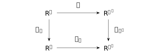
The lower map exists because the retained subset is transported. Keeping the target labels fixed can select an inequivalent marginal; the adjacent-versus-opposite example gives both the precision calculation and a failure of projection factorization.
These conclusions use positive precisions and the stated product volumes. Fixing an eliminated field, taking a conditional-density kernel, and taking a marginal are different operations. A singular full-fiber integral is not repaired by a pseudoinverse: changing the integration space changes the measure. The massless projected cycle law has its proved density on the specified retained image, and is not obtained by inserting a mean-zero constraint into the unconstrained marginal formula.
[friedli2017statistical, Proposition B.55, p. 505] gives the Gaussian change-of-variables convention.
[tao2011measure, Theorem 1.7.15, pp. 200-202] gives the nonnegative integration convention on the Borel product measures; absolute integrability precedes signed subtraction.
[boyd2004convex, Appendix A.5.5, pp. 650-651] gives the real block convention, with its first pivot exchanged to \(C\).
Mathlib's LinearIsometryEquiv.measurePreserving
supplies volume preservation for finite-dimensional real linear
isometry equivalences. TauCeti's
TauCeti.Probability.map_affine_multivariateGaussian
supplies covariance-parameter transport. Set mean and shift to zero,
linear map to \(P\), and covariance to \(Q^{-1}\); the
precision-density identification and the proved inverse
identity align it with this law. These interfaces do not supply the
endpoint data, declared partition or its counterexample.
Theorem 10.9. Symmetry survives the Gaussian marginal [fdip-000K]AGENTDRAFTED
- October 17, 2026
Theorem 10.9. Symmetry survives the Gaussian marginal [fdip-000K]AGENTDRAFTED
- October 17, 2026
Let a group \(\Gamma \) act by a signed-incidence symmetry on a finite incidence presentation with positive real weights and nonempty vertex set. Use the counting pairings, their induced Borel volume and a scalar mass \(m>0\). The positive massive precision and inverse-precision covariance are \[L=d^\dagger Wd,\qquad Q=L+m^2I,\qquad G=Q^{-1}.\] For every \(g\in \Gamma \), \[\begin {aligned} LP_g&=P_gL,&QP_g&=P_gQ,\\ GP_g&=P_gG,&P_gGP_g^\dagger &=G. \end {aligned}\] Thus \(Qf=j\) implies \(Q(P_gf)=P_gj\). The Gaussian law is invariant: \((P_g)_*\mu _Q=\mu _Q\). For every real or complex Borel observable \(F\), \[\begin {aligned} \int |F\circ P_g|\,d\mu _Q&=\int |F|\,d\mu _Q,\\ \omega _Q(F\circ P_g)&=\omega _Q(F) \end {aligned}\] with extended integrals in the first equality, and finite absolute integral required in the second.
Proof.
- October 17, 2026
Proof.
- October 17, 2026
The signed action gives counting isometries and \(dP_g=J_gd\), \(WJ_g=J_gW\). The paired transport theorem gives the stated commutations; \(P_g^\dagger =P_g^{-1}\) gives the covariance congruence. The unique sourced solution is \(f=Gj\). At zero source this is zero, although the action on the entire field carrier need not be trivial.
The scalar Euclidean action \(\mathcal A_Q(f)=b(f,Qf)/2\) satisfies \(\mathcal A_Q(P_gf)=\mathcal A_Q(f)\) by pairing isometry and commutation. This scalar function differs from the group action \(g\mapsto P_g\). The Gaussian transport theorem, with \(Q'=Q\), proves event-law invariance and the extended absolute integral before the expectation assertion. Its proof applies to the weaker incidence intertwiners and therefore to signed endpoint actions; no directed-endpoint claim is inferred from the weaker hypotheses.
Suppose further that a nonempty proper retained subset \(R\subsetneq V\) is stable under every \(p_g\). Its complement \(D=V\setminus R\) is also stable. The restricted maps \(P_{g,R},P_{g,D}\) give the orthogonal split correspondence. For the split components \(A,B,E,C\), with \(E=B^\dagger \), and \(S=A-BC^{-1}E>0\), one has \[\begin {aligned} P_{g,R}SP_{g,R}^{-1}&=S,\\ P_{g,R}S^{-1}P_{g,R}^{-1}&=S^{-1},\\ (P_{g,R})_*\mu _S&=\mu _S. \end {aligned}\] The retained equation \(Sx=k\) is equivariant as well. The full fiber factor \(c_C=(2\pi )^{|D|/2}/\sqrt {\det C}\) and the stationary eliminated field are compatible with the action: \[y_*(P_{g,R}x)=P_{g,D}y_*(x),\qquad y_*(x)=-C^{-1}Ex.\]
Proof.
- October 17, 2026
Proof.
- October 17, 2026
The four-block transport identities give Schur conjugacy, its inverse conjugacy, and stationary-field transport. Its actual projection identity is \(\pi _RP_g=P_{g,R}\pi _R\). By the normalized marginal theorem and full-law invariance, \[\begin {aligned} (P_{g,R})_*\mu _S &=(P_{g,R}\pi _R)_*\mu _Q\\ &=(\pi _RP_g)_*\mu _Q=\pi _{R*}\mu _Q=\mu _S. \end {aligned}\] The real transport theorem also proves invariance of \(\det C\), \(c_C\), the additive action constant and \(Z_S\). For every integrable retained observable \(f\), \[\begin {aligned} \omega _S(f\circ P_{g,R})&=\omega _S(f),\\ \omega _Q(f\circ \pi _R)&=\omega _S(f). \end {aligned}\] The marginal theorem supplies the absolute-integral equivalence needed here. On actual polynomial functions this is the retained functional square. Gaussian integration proves the law; algebraic Schur conjugacy by itself does not.
For the half-turn, retain \(R=(0,2)\) and eliminate \(D=(1,3)\). Both restrictions are the nonidentity swap \(J=\begin {pmatrix}0&1\\1&0\end {pmatrix}\). Here \(H\) is the array of the split component \(B\). The projection square is
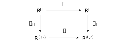
The lower map swaps the two retained coordinates. Put \(a=m^2\) and \(s=1+t+a\). The explicit elimination gives \[\begin {aligned} A=C&=sI_2,\qquad H=-\begin {pmatrix}1&t\\t&1\end {pmatrix},\\ S&=\begin {pmatrix}\alpha &-\beta \\-\beta &\alpha \end {pmatrix},\\ \alpha &=s-\frac {1+t^2}{s},\qquad \beta =\frac {2t}{s}. \end {aligned}\] All three blocks commute with \(J\), hence \(JSJ=S\). Positivity follows also from the two eigenvalues \[\begin {aligned} \alpha -\beta &=\frac {a(a+2+2t)}s>0,\\ \alpha +\beta &=\frac {(a+2)(a+2t)}s>0. \end {aligned}\] Thus the same nontrivial action preserves the full and retained laws. The full covariance obeys \(G_{i+2,j+2}=G_{ij}\). Invariant state does not mean that each observable is pointwise invariant: \(\phi \mapsto \phi _0^2\) is sent to \(\phi \mapsto \phi _2^2\); they differ at \(\delta _0\), but their expectations agree.
At \(t=m=1\), direct inversion gives \[\begin {aligned} S&=\begin {pmatrix}7/3&-2/3\\-2/3&7/3\end {pmatrix},\\ S^{-1}&=\begin {pmatrix}7/15&2/15\\2/15&7/15\end {pmatrix}. \end {aligned}\] Both swapped squared coordinates have expectation \(7/15\). The observable \(\phi _0\phi _2\) is itself invariant under the half-turn and has expectation \(2/15\). These expectations agree before and after elimination.
The full and retained half-turns are both faithful: their nonidentity maps send \(\delta _0\) to \(\delta _2\). A general full faithful action can restrict trivially, for instance when it moves only eliminated vertices. These two assertions are compatible.
Three concrete obstructions distinguish the hypotheses: keeping fixed target labels after relabeling, breaking the alternating weights, and choosing a nonstable retained subset. The last is a failure of descent through that projection and does not exclude accidental symmetry of a marginal density. Extra mass fields or reference pairings would require their own preservation hypotheses.
[milne2025group, Definition 4.1 and p. 58] gives the group-action and stable-subset conventions.
[friedli2017statistical, Proposition B.55, p. 505] gives the Gaussian substitution convention. The incidence, stationary and half-turn computations above use the proved transport results and the exact cycle elimination.
Mathlib's LinearIsometryEquiv.measurePreserving
supplies isometry-volume preservation. TauCeti's
TauCeti.Probability.map_affine_multivariateGaussian
supports covariance-parameter pushforward for the supplied \(P_g\)
or retained projection after the precision-density bridge.
These declarations do not assert the endpoint, weight or stable-subset
hypotheses, or the concrete failures just cited.
Example 10.10. Fixed labels can select a different marginal [fdip-003J]AGENTDRAFTED
- October 29, 2026
Example 10.10. Fixed labels can select a different marginal [fdip-003J]AGENTDRAFTED
- October 29, 2026
A global relabeling need not preserve a marginal requested on fixed labels. In the four-cycle, take \(t=m=1\) and retain \(R=\{0,2\}\). Its effective precision is \[S_{\mathrm {opp}}= \begin {pmatrix}7/3&-2/3\\-2/3&7/3\end {pmatrix}.\] Exchange labels \(1,2\), fixing \(0,3\), and form \(Q'=PQP^T\). If the new retained labels are still \(\{0,2\}\), they select the original adjacent variables \(\{0,1\}\). In the old coordinate order \((0,1)\mid (2,3)\), the relevant blocks are \[\begin {aligned} A=C&=\begin {pmatrix}3&-1\\-1&3\end {pmatrix},\\ H&=\begin {pmatrix}0&-1\\-1&0\end {pmatrix},\\ C^{-1}=HC^{-1}H^T &=\frac 18\begin {pmatrix}3&1\\1&3\end {pmatrix}. \end {aligned}\] Subtraction gives \[S_{\mathrm {adj}}= \begin {pmatrix}21/8&-9/8\\-9/8&21/8\end {pmatrix}.\] The diagonal entries \(7/3\) and \(21/8\) differ, so no two-coordinate permutation conjugates these precisions. There is also no map on the old retained fields factoring \(\pi _RP\) through \(\pi _R\): the fields \(0\) and \(\delta _1\) have the same old projection, but their projections after \(P\) are \(0\) and \((0,1)\). Here \(\delta _1\) is the delta field at vertex \(1\), not the edge label \(e_1\). Transporting the retained subset to \(p(R)=\{0,1\}\) in the new labels restores the square and the marginal transport theorem.
The blocks are a direct calculation from the alternating-cycle precision, using the Schur convention of [boyd2004convex, Appendix A.5.5, pp. 650-651] after exchanging its first pivot to \(C\). The example separates a fixed set of labels from the moving retained space required by Proposition 10.5.
Example 10.11. Breaking the weights breaks the half-turn [fdip-003K]AGENTDRAFTED
- October 29, 2026
Example 10.11. Breaking the weights breaks the half-turn [fdip-003K]AGENTDRAFTED
- October 29, 2026
In the alternating four-cycle, take \(t,m>0\) and the half-turn. It fails to preserve the action after a specific positive change of weights. Replace \((1,t,1,t)\) by \((1,t,2,t)\) while keeping the proposed half-turn. Then \(L_{00}=1+t\) and \(L_{22}=2+t\), so \(PLP^T\ne L\) and \(\mathcal A(\delta _2)-\mathcal A(\delta _0)=1/2\). If its Gaussian law were invariant, second moments would give \(PGP^T=G\); inversion would give \(PQP^T=Q\), contradicting those diagonal entries. At \(t=m=1\), retain the opposite pair \(R=(0,2)\) and eliminate \(D=(1,3)\). The blocks in that order are \[\begin {aligned} A=C&=\operatorname {diag}(3,4),\\ H&=-\begin {pmatrix}1&1\\1&2\end {pmatrix},\\ S_{\mathrm {broken}} &=\begin {pmatrix}29/12&-5/6\\-5/6&8/3\end {pmatrix}. \end {aligned}\] Indeed \[HC^{-1}H^T=\begin {pmatrix}7/12&5/6\\5/6&4/3\end {pmatrix},\] and subtracting from \(A\) gives the displayed precision. Its diagonal entries differ by \(1/4\), so its marginal also fails swap invariance. Its positive Gaussian still exists.
[spielman2009effective, Section 2.1, pp. 4-5] gives the edge-once convention.
[boyd2004convex, Appendix A.5.5, pp. 650-651] gives the positive Gaussian elimination convention. The action difference and matrix products are direct calculations with these conventions. Weight preservation is sufficient in the general transport theorem; it need not be necessary for every presentation with redundant loops or parallel edges. This example establishes failure for the stated weights, not a universal necessity.
Example 10.12. A nonstable retained set need not inherit the action [fdip-003L]AGENTDRAFTED
- October 29, 2026
Example 10.12. A nonstable retained set need not inherit the action [fdip-003L]AGENTDRAFTED
- October 29, 2026
In the alternating four-cycle with weights \((1,t,1,t)\) and \(t,m>0\), consider the half-turn and the adjacent retained subset \(R=\{0,1\}\). The half-turn preserves the full state, but sends \(R\) to \(D=\{2,3\}\). No map \(T\) of retained fields can satisfy \(\pi _RP=T\pi _R\): the zero field forces \(T(0)=0\), while \(\delta _2\) has retained projection zero and projects to \((1,0)\) after the half-turn. The action transports the marginal to a different subset; it does not descend through this fixed projection. This does not exclude accidental symmetries of an individual two-site density. A general restricted action may also be trivial, unlike the opposite-pair swap. Extra mass fields or reference pairings would require their own preservation hypotheses.
The stable-subset requirement is the equivariance convention of [milne2025group, p. 58]. The two-field witness proves failure of factorization even through a nonlinear function. It differs from the fixed-label relabeling failure: here the full half-turn symmetry is unchanged, and the chosen projection fails to admit its action. The moving square of Proposition 10.5 remains valid on \(\mathbb R^{pR}\). Over any nonzero commutative unital coefficient ring \(k\), the same delta-field witness works on \(k^V\); over the zero ring all fields coincide.
Definition 10.13. Intrinsic trace on a finite free module [fdip-003G]AGENTDRAFTED
- October 29, 2026
Definition 10.13. Intrinsic trace on a finite free module [fdip-003G]AGENTDRAFTED
- October 29, 2026
A trace can be defined before choosing a pairing or displaying a matrix. Let \(k\) be a commutative unital ring and \(M\) a finite free \(k\)-module. A finite dual frame is a finite family \(m_i\in M\), \(\ell _i\in M^\vee \) such that \[x=\sum _i\ell _i(x)m_i\qquad (x\in M).\] A basis and its coefficient functionals supply such a frame; the counting carrier \(k^V\) uses its delta dual frame. For an endomorphism \(T:M\to M\), define its intrinsic trace by \[\operatorname {tr}_M(T)=\sum _i\ell _i(Tm_i).\] This scalar is independent of the frame. It is linear in \(T\), and for maps between finite free modules \(f:M\to N\), \(g:N\to M\), \[\operatorname {tr}_M(gf)=\operatorname {tr}_N(fg).\] In particular, for an isomorphism \(P:M\to M'\), \[\operatorname {tr}_{M'}(PTP^{-1})=\operatorname {tr}_M(T).\]
Proof.
- October 29, 2026
Proof.
- October 29, 2026
Let \(n_j,\psi _j\) be another dual frame of \(M\). Expanding \(m_i\) in this frame and commuting the scalars in \(k\) gives \[\begin {aligned} \sum _i\ell _i(Tm_i) &=\sum _{i,j}\psi _j(m_i)\ell _i(Tn_j)\\ &=\sum _j\psi _j(Tn_j). \end {aligned}\] For the last equality, evaluate \(\sum _i\psi _j(m_i)\ell _i(x)=\psi _j(\sum _i\ell _i(x)m_i)=\psi _j(x)\) at \(x=Tn_j\). This proves frame independence without a pairing. Termwise addition and scalar multiplication give \(\operatorname {tr}(T+U)=\operatorname {tr}(T)+\operatorname {tr}(U)\) and \(\operatorname {tr}(cT)=c\operatorname {tr}(T)\).
Take dual frames \(m_i,\ell _i\) for \(M\) and \(n_j,\psi _j\) for \(N\). Expanding \(fm_i\) and \(gn_j\) gives \[\begin {aligned} \operatorname {tr}_M(gf) &=\sum _{i,j}\psi _j(fm_i)\ell _i(gn_j)\\ &=\operatorname {tr}_N(fg). \end {aligned}\] This is rectangular cyclicity; the two traces may be on different modules. The transported family \(Pm_i,\ell _iP^{-1}\) is a dual frame of \(M'\). Substitution into the defining sum proves the conjugacy formula.
With a basis, \(\ell _i(Tm_i)\) is the \(i\)-th diagonal coefficient, so coordinate trace is recovered as \(\sum _iT_{ii}\). For the zero module the empty frame gives trace zero; the same formulas also make sense over the zero ring. The declared category here is finite free modules. No totalized trace on arbitrary modules and no finite-projective extension are needed.
The duality/evaluation convention is [stacks2017stacks, More on Algebra, Lemma 74.1], Tag 0FNJ. [stacks2017stacks, Exercises, Exercise 22.6], Tag 02DU asks for trace, naturality and cyclicity on finite locally free modules; the finite-free proof above is supplied here, rather than attributed to a proof in that exercise.
Mathlib's LinearMap.trace has a totalized definition.
On the finite-free commutative-ring domain, its
LinearMap.trace_comp_comm' is rectangular cyclicity and
LinearMap.trace_conj' is conjugacy by a linear equivalence.
The definition above uses only this finite-free domain.
Matrix.trace_mul_comm expresses the coordinate rectangular
identity; a trace pairing is not an assumption of either construction.
Proposition 10.14. The trace ratio on its unit-denominator domain [fdip-003H]AGENTDRAFTED
- October 29, 2026
Proposition 10.14. The trace ratio on its unit-denominator domain [fdip-003H]AGENTDRAFTED
- October 29, 2026
Let \(L:M\to M\) be an endomorphism of a finite free module over a commutative unital ring \(k\). On the domain \(\operatorname {tr}_M(L)\in k^\times \), define the trace ratio \[R(L)=\operatorname {tr}_M(L^2)\bigl (\operatorname {tr}_M(L)\bigr )^{-2},\] using intrinsic trace. If \(P:M\to M'\) is an isomorphism, \(c\in k^\times \), and \(L'=cPLP^{-1}\), then \(\operatorname {tr}_{M'}(L')\) is a unit and \(R(L')=R(L)\).
Proof.
- October 29, 2026
Proof.
- October 29, 2026
Put \(a=\operatorname {tr}_M(L)\). Linearity, conjugacy and \((L')^2=c^2PL^2P^{-1}\) give \[\begin {aligned} \operatorname {tr}_{M'}(L')&=ca,\\ \operatorname {tr}_{M'}((L')^2)&=c^2\operatorname {tr}_M(L^2). \end {aligned}\] Both \(c\) and \(a\) are units, so \(ca\) is a unit with inverse \(a^{-1}c^{-1}\). Substitution cancels \(c^2\) from the ratio.
Consider a finite-dimensional positive inner-product space over \(\mathbb R\). A nonzero self-adjoint positive-semidefinite operator on it has positive trace. Indeed an orthonormal eigenbasis gives eigenvalues \(\lambda _i\geq 0\); if all were zero the operator would be zero. Hence \(\operatorname {tr}L=\sum _i\lambda _i>0\). This verifies the denominator for a nonzero positive-weight graph Laplacian.
[boyd2004convex, Appendix A.5.2, pp. 646-647] gives the spectral and trace formulas. The exceptional examples show why nonzero alone is insufficient over other rings or without positivity.
For nonzero real positive-semidefinite Laplacians with their counting pairings, write \(L\approx L'\) when \(L'=cPLP^{-1}\) for a positive scalar and a vertex permutation. Identity uses \((1,I)\); inverse uses \((c^{-1},P^{-1})\); composition uses the products of the scalars and permutations. This is an equivalence relation with invariant \(R\). It forgets the mass, normalized state and retained partition of an enriched background. It also differs from arbitrary congruence of bilinear-form arrays: the ratio compares the associated endomorphisms. It is an invariant, not a classification assertion.
The ring calculation is a direct consequence of Definition 10.13,
whose trace convention is
[stacks2017stacks, Exercise 22.6], Tag 02DU.
Mathlib's Matrix.trace_smul supplies the coordinate scalar
identity; the unit domain and cancellation above are additional
hypotheses and deductions. The cycle comparison computes
the invariant and the associated normalized observables explicitly.
Example 10.15. Nonzero operators outside the trace-ratio domain [fdip-003I]AGENTDRAFTED
- October 29, 2026
Example 10.15. Nonzero operators outside the trace-ratio domain [fdip-003I]AGENTDRAFTED
- October 29, 2026
The unit condition in the trace ratio distinguishes several elementary cases. For one unit-weight edge on two vertices, the Laplacian over \(\mathbb Z\) is \[L=\begin {pmatrix}1&-1\\-1&1\end {pmatrix}.\] Its trace is \(2\), which is not a unit in \(\mathbb Z\); the defining formula therefore does not give a \(\mathbb Z\)-valued ratio. After inverting \(2\) it does: \(L^2=2L\) gives ratio \(1\). Reduction over \(\mathbb F_2\) instead gives the nonzero matrix \[\overline L=\begin {pmatrix}1&1\\1&1\end {pmatrix},\] whose trace is zero and whose square is zero. Nonzero incidence energy as an algebraic operator does not imply a unit trace.
Over \(\mathbb R\), the nonzero self-adjoint matrix \(\operatorname {diag}(1,-1)\) has trace zero. It is not positive semidefinite, so it does not contradict the positive-trace proof. For an incidence presentation containing only loops, \(d=0\) and \(L=d^\dagger Wd=0\); the trace is zero whatever the loop weights. The empty carrier likewise has zero trace by the empty dual-frame sum. In each case the ratio is undefined over a nonzero ring.
In the zero ring, \(0=1\) is its sole unit, and every unital module and scalar has one element. The formula for the ratio then has the unique value \(0\). This algebraic convention makes no assertion about a nonzero positive-real Laplacian.
[spielman2009effective, Section 2.1, pp. 4-5] gives the edge-once incidence convention used here, as extended algebraically in Definition 10.1. These computations also use the directly proved dual-frame trace.
[boyd2004convex, Appendix A.5.2, pp. 646-647] gives the spectral criterion for the real positivity boundary. The ring reductions and zero-ring conclusion are the explicit calculations here, not probability statements from those sources.
Example 10.16. A trace ratio separates two weighted cycles [fdip-000I]AGENTDRAFTED
- October 17, 2026
Example 10.16. A trace ratio separates two weighted cycles [fdip-000I]AGENTDRAFTED
- October 17, 2026
The alternating cycles at \(t=1\) and \(t=2\) remain different even under the positive-scaling Laplacian comparison \(L'=cPLP^{-1}\), with \(c>0\) and \(P\) a vertex permutation. Use the trace ratio \[R(L)=\frac {\operatorname {tr}(L^2)}{(\operatorname {tr}L)^2},\] where the trace is the intrinsic endomorphism trace. The positive graph energy gives a nonzero positive-semidefinite \(L_t\) for \(t>0\), so its trace is positive and the ratio is defined. The cited proposition proves invariance by trace conjugacy and scalar cancellation. It compares counting-relative operators, not bilinear-form arrays under arbitrary congruence.
[boyd2004convex, Appendix A.5.2, pp. 646-647] gives the symmetric spectral and trace formulas. The spectral cycle calculation supplies the concrete basis; the following traces and comparisons are direct computations.
For the alternating four-cycle, \(t>0\), the orthonormal spectral basis gives eigenvalues \(0,2,2t,2+2t\), including at \(t=1\). Consequently \[\begin {aligned} \operatorname {tr}L_t&=4(1+t),\\ \operatorname {tr}(L_t^2) &=4+4t^2+4(1+t)^2\\ &=8(t^2+t+1),\\ R(t):=R(L_t)&=\frac {t^2+t+1}{2(t+1)^2}. \end {aligned}\] In particular \[\begin {aligned} R(1)&=\frac 38,\qquad R(2)=\frac 7{18},\\ R(2)-R(1)&=\frac 1{72}>0. \end {aligned}\] There can be no \(c>0\) and vertex permutation \(P\) with \(L_2=cPL_1P^T\). Thus the associated finite Gaussian backgrounds cannot be exactly relabeled into each other either. This calculation separates the stated pair; it does not claim a classification of all backgrounds.
The reciprocal identity \(R(t)=R(1/t)\) is consistent with this comparison. A one-step rotation \(p(i)=i+1\pmod 4\) exchanges the alternating edge weights \(1,t\) and leaves the common diagonal \(1+t\) unchanged. Its coordinate permutation therefore satisfies \[PL_tP^T=tL_{1/t}.\] Since \(1/t>0\), the reciprocal Laplacians are equivalent under \(\approx \). Their equal ratios do not demonstrate a failure of completeness. On the strict enriched slice with weights \((1,t,1,t)\), fixed mass and fixed opposite retained pair, the weight product is \(t^2\), whereas at parameter \(1/t\) it is \(t^{-2}\). A weight-preserving edge bijection would preserve this product; for positive \(t\) equality forces \(t=1\). Thus the broader reciprocal comparison is not a strict background isomorphism for \(t\ne 1\).
A fixed-mass calculation shows what changes in the induced state. Set \(m=1\) and retain the same labeled vertices \(R=\{0,2\}\). The alternate-vertex elimination has \(s=t+2\), giving \[\begin {aligned} \alpha (t)&=s-\frac {1+t^2}{s}=\frac {4t+3}{t+2},\\ \beta (t)&=\frac {2t}{t+2},\\ S_t&=\begin {pmatrix}\alpha (t)&-\beta (t)\\ -\beta (t)&\alpha (t)\end {pmatrix}. \end {aligned}\] Hence the effective coupling changes from \(\beta (1)=2/3\) to \(\beta (2)=1\), and the two precisions are \[\begin {aligned} S_1&=\begin {pmatrix}7/3&-2/3\\-2/3&7/3\end {pmatrix},\\ S_2&=\begin {pmatrix}11/4&-1\\-1&11/4\end {pmatrix}. \end {aligned}\] Their determinants are \(5\) and \(105/16\). The off-diagonal entry of \(S_t^{-1}\) is \(\beta (t)/\det S_t\). By the marginal expectation identity, the same labeled observable therefore has different normalized expectations: \[\begin {aligned} \langle \phi _0\phi _2\rangle _{t=1,m=1}&=\frac {2}{15},\\ \langle \phi _0\phi _2\rangle _{t=2,m=1}&=\frac {16}{105}. \end {aligned}\] This comparison fixes the mass, coordinates, reference pairing and partition. The labeled observable is not itself asserted invariant under every relabeling; the trace ratio already established the broader inequivalence.
Scale invariance of \(R\) does not mean equality of fixed-mass states. On an eigenvector of \(L\) with eigenvalue \(\lambda >0\), replacing \(L\) by \(cL\) changes the covariance eigenvalue from \(1/(\lambda +m^2)\) to \(1/(c\lambda +m^2)\) when \(c\ne 1\). Scaling all of \(Q\) instead gives covariance \(c^{-1}G\) and Schur map \(cS\), by inversion and the Schur formula. Changing mass can also leave \(R(L)\) unchanged while changing the law. The exact finite differences above do not construct a physical map from an environment to the parameter \(t\).
The trace identities and their formalization correspondence are at Definition 10.13 and Proposition 10.14. Their unit-domain hypotheses specialize here to positive real trace; the values and normalized expectation comparisons above are additional cycle calculations.
Proposition 10.17. Jacobian compensation in normalized Gaussian transport [fdip-003M]AGENTDRAFTED
- October 29, 2026
Proposition 10.17. Jacobian compensation in normalized Gaussian transport [fdip-003M]AGENTDRAFTED
- October 29, 2026
Let \(M,M'\) be finite-dimensional real positive inner-product spaces with induced Borel Euclidean volumes \(\lambda ,\lambda '\). Let \(Q,Q'\) be positive self-adjoint precisions, and suppose a linear isomorphism \(T:M\to M'\) preserves their actions: \[\mathcal A_{Q'}(Tx)=\mathcal A_Q(x).\] It need not preserve the reference pairings. For its absolute Jacobian \(J(T)>0\), one has \[\begin {aligned} T_*\lambda &=J(T)^{-1}\lambda ',\\ Z_{Q'}&=J(T)Z_Q,\qquad T_*\mu _Q=\mu _{Q'}. \end {aligned}\] For every real or complex Borel observable \(F'\), \[\int |F'|\,d\mu _{Q'}=\int |F'\circ T|\,d\mu _Q\] as extended nonnegative integrals. Hence integrability is equivalent on the two sides, and, under that condition, \(\omega _{Q'}(F')=\omega _Q(F'\circ T)\).
Proof.
- October 29, 2026
Proof.
- October 29, 2026
The reference-volume change formula gives the pushforward of volume, equivalently \(\int h'\,d\lambda '=J(T)\int h'\circ T\,d\lambda \) for every nonnegative Borel \(h'\). Apply it to the Gaussian weight; action preservation gives \(Z_{Q'}=J(T)Z_Q\). Both normalizers are finite and positive by Theorem 7.7. For a nonnegative Borel \(h'\), divide the same substitution by this equality: \[\begin {aligned} \int h'\,d\mu _{Q'} &=\frac {J(T)}{Z_{Q'}}\int h'(Tx)e^{-\mathcal A_Q(x)}\,d\lambda (x)\\ &=\int h'\circ T\,d\mu _Q. \end {aligned}\] Indicators of Borel sets prove the event-pushforward statement. Taking \(h'=|F'|\) proves the extended absolute-integral equality. Only when finite do positive/negative parts, and for complex functions real/imaginary parts, give the stated expectation identity.
In orthonormal coordinates, action preservation means \(T^TQ'T=Q\), so inversion gives \[(Q')^{-1}=TQ^{-1}T^T.\] This is covariance congruence, not generally operator similarity. The scalar Jacobian is computed in the specified reference volumes; independently ordered orthonormal frames may change the signed determinant but not its absolute value. The quadratic-isometry example shows that this normalized transport can lose both counting-pairing and retained-projection compatibility. Such maps are not enriched background arrows.
The volume convention is
[tao2011measure, Exercises 1.2.20-22, p. 41]; the covariance-parameter
Gaussian substitution is
[friedli2017statistical, Proposition B.55, p. 505].
The inverse-precision covariance theorem identifies its
covariance with \(Q^{-1}\) for these reference pairings.
TauCeti's
TauCeti.Probability.map_affine_multivariateGaussian
supports the covariance congruence for a supplied finite real linear
map, even rectangular. That broader covariance result does not assert
invertibility, endpoint preservation or the retained square used here.
11. Group-algebra sectors [fdip-001A]AGENTDRAFTED
- October 20, 2026
11. Group-algebra sectors [fdip-001A]AGENTDRAFTED
- October 20, 2026
How can the same half-turn act on different Gaussian states? The group-algebra extension and its module projectors separate the actual half-turn sectors whenever two is invertible. The action and its projectors are specified before a probability law is attached. Support parity and sign sectors are different decompositions of the same fields.
Over the reals, an orthogonal involution commuting with positive precision gives a product law; the four-cycle calculation computes its two blocks and retained marginals. Symmetry still permits mixing within a sector, and in characteristic two the action survives without the complementary projectors. These examples separate the supplied symmetry, the coefficient assumptions and the choice of state.
Theorem 11.1. Extending a group action on a ring module [fdip-003N]AGENTDRAFTED
- October 29, 2026
Theorem 11.1. Extending a group action on a ring module [fdip-003N]AGENTDRAFTED
- October 29, 2026
Let \(k\) be a commutative unital ring, \(G\) a group and \(M\) a unital \(k\)-module. A linear action \(\rho :G\to \operatorname {Aut}_k(M)\) extends uniquely to a unital \(k\)-algebra homomorphism \[\widehat \rho :k[G]\longrightarrow \operatorname {End}_k(M),\qquad \widehat \rho \left (\sum _g a_g[g]\right )=\sum _g a_g\rho (g).\] Products of endomorphisms compose right to left. This extends the Group Algebra universal property to the actual module action; no finiteness of \(G\) is assumed.
Proof.
- October 29, 2026
Proof.
- October 29, 2026
Elements of \(k[G]\) are finite-support functions on \(G\). The coefficient of \([u]\) in a product is \(\sum _{gh=u}a_gb_h\); only pairs in the finite set \(\operatorname {supp}(a)\times \operatorname {supp}(b)\) contribute. Its image under multiplication contains the product support. Associativity follows by reassociating the finite triple sum and using \((gh)j=g(hj)\). The unit is \([1_G]\), and the scalar \(c[1_G]\) commutes with every basis element. Thus these formulas define a unital \(k\)-algebra, including for the zero ring.
The displayed extension is additive and \(k\)-linear. Moreover \[\begin {aligned} \widehat \rho (ab)&=\sum _{g,h}a_gb_h\rho (gh)\\ &=\sum _{g,h}a_gb_h\rho (g)\rho (h) =\widehat \rho (a)\widehat \rho (b). \end {aligned}\] The \(k\)-linearity of each \(\rho (g)\) moves coefficients through it; the order of \(g,h\) is unchanged. The extension sends \([1_G]\) to \(I_M\) and \(c[1_G]\) to \(cI_M\). Every linear extension has this value on each finite basis expansion, proving uniqueness. In the regular action, \(\rho (g)\rho (h)\) first multiplies \([1_G]\) by \([h]\), then by \([g]\), giving \([gh]\). For \(g=(12),h=(23)\) in \(S_3\), this differs from \([hg]\) when \(k\ne 0\). The nonzero assumption is needed only for this distinguishing witness.
Consequently linear \(G\)-actions correspond to unital left \(k[G]\)-module structures whose restriction along \(c\mapsto c[1_G]\) is the given scalar action. Under this correspondence, a \(k\)-linear map \(f:M\to N\) is a module map exactly when \(f\rho _M(g)=\rho _N(g)f\) for every \(g\).
Proof.
- October 29, 2026
Proof.
- October 29, 2026
Define \(a\cdot m=\widehat \rho (a)m\); linearity, multiplication and the unit just proved give the module laws. Conversely, restrict a \(k[G]\)-module to \(k\) and set \(\rho (g)m=[g]m\). Centrality of scalars gives \(k\)-linearity, \([g^{-1}]\) gives the inverse, and \([gh]=[g][h]\) gives the representation law. Finite distributivity shows that the two constructions are inverse. This scalar restriction is essential; an unrelated \(k\)-module structure is not being identified.
If \(f\) intertwines the group elements, finite linearity gives \[f\widehat \rho _M(a)m =\sum _g a_g f\rho _M(g)m =\sum _g a_g\rho _N(g)fm =\widehat \rho _N(a)fm.\] The converse follows by taking \(a=[g]\). This proves intertwining for every algebra element, including scalars and the unit.
[sengupta2010representations, Sections 3.1-3.2, pp. 39-41]
presents the field case, with finite support for an arbitrary group.
The proof above is the ring adaptation of
representation/module correspondence.
Mathlib's Representation.asAlgebraHom and
Representation.asAlgebraHom_single supply the linear extension
and its value on basis monomials. They do not assert that an arbitrary
faithful group action has a faithful algebra extension. For example,
\(C_2\to \mathbb R^\times \), \(r\mapsto -1\), is injective, but its
algebra extension annihilates the nonzero element \(1+[r]\).
Theorem 11.2. Projectors of an involution on a module [fdip-003O]AGENTDRAFTED
- October 29, 2026
Theorem 11.2. Projectors of an involution on a module [fdip-003O]AGENTDRAFTED
- October 29, 2026
Let \(k\) be a commutative unital ring in which \(2\) is a unit, put \(h=2^{-1}\), and let \(T:M\to M\) be linear with \(T^2=I\). The maps \(E_\varepsilon =h(I+\varepsilon T)\), for \(\varepsilon \in \{1,-1\}\), give \[\begin {aligned} E_\varepsilon ^2&=E_\varepsilon ,&E_+E_-&=E_-E_+=0,\\ E_++E_-&=I,&E_+-E_-&=T,\\ \operatorname {im}E_\varepsilon &=\ker (T-\varepsilon I)=M_\varepsilon . \end {aligned}\] Thus \(M\cong M_+\oplus M_-\), with map \(v\mapsto (E_+v,E_-v)\) and inverse addition. No finite generation, freeness or pairing is needed.
Proof.
- October 29, 2026
Proof.
- October 29, 2026
Scalar maps commute with \(T\), so \[E_\varepsilon ^2=h^2(I+2\varepsilon T+T^2) =2h^2(I+\varepsilon T)=E_\varepsilon .\] Both mixed products equal \(h^2(I-T^2)=0\); sum and difference use \(2h=1\). Also \(TE_\varepsilon =\varepsilon E_\varepsilon \). If \(Tv=\varepsilon v\), then \(E_\varepsilon v=h(v+v)=v\), proving equality of image and eigenspace. The sum identity decomposes every vector. If \(u_++u_-=0\) with \(u_\pm \in M_\pm \), applying \(E_+\) gives \(u_+=0\), and then \(u_-=0\), proving uniqueness.
If an algebra acts by \(\alpha :A\to \operatorname {End}_k(M)\), these projectors are \(A\)-linear precisely when \[T\alpha (a)=\alpha (a)T\qquad (a\in A).\] Indeed this is exactly \(A\)-linearity of \(T\); its linear combinations with \(I\) are then \(A\)-linear. Conversely, either projector recovers \(T=2E_+-I=I-2E_-\). When \(T=\alpha (\omega )\), centrality of \(\omega \) is sufficient. It need not be necessary: on \(M=\mathbb R\), let \(A=\mathbb R\times M_2(\mathbb R)\) act by \(\alpha (a,B)=aI\), and put \(\omega =(1,\operatorname {diag}(1,-1))\). Then \(\omega ^2=1\) and \(T=I\), although \(\omega \) fails to commute with a matrix unit in the second factor.
For comparison, the central-idempotent product is an algebra statement. Central orthogonal idempotents \(e_+,e_-\) with sum one give the mutually inverse unital algebra maps \[a\longmapsto (e_+a,e_-a),\qquad (x,y)\longmapsto x+y.\] Each ideal \(e_\varepsilon A\) has unit \(e_\varepsilon \) and scalar map \(c\mapsto ce_\varepsilon \). Centrality makes each component multiplicative and the mixed products zero; the sum and orthogonality identities prove both inverse equations. This is stronger than the module splitting above.
In \(k[C_2]\), writing \(g=[r]\) for \(r^2=1\), the two central idempotents are \(e_\pm =h(1\pm g)\). The explicit product is \[\begin {aligned} \Phi (a+bg)&=(a+b,a-b),\\ \Phi ^{-1}(x,y)&=h(x+y)+h(x-y)g. \end {aligned}\] The coefficient product \((a+bg)(c+dg)=(ac+bd)+(ad+bc)g\) maps to \(((a+b)(c+d),(a-b)(c-d))\). Thus \(\Phi \) is multiplicative; its inverse equations use \(2h=1\), its unit image is \((1,1)\), and scalars map diagonally. The images of \(e_+,e_-\) are \((1,0),(0,1)\). An arbitrary coefficient ring need not be semisimple, and an abstract idempotent summand need not be free.
[sengupta2010representations, Section 4.5, pp. 63-64]
discusses character projectors over a field with invertible group order;
its subsequent ideal argument assumes semisimplicity. The displayed
ring identities require only invertible two. Mathlib's
LinearMap.IsIdempotentElem.isCompl supplies the abstract
range/kernel complement. TauCeti's
TauCeti.isIdempotentElem_halfOneAdd supplies the
square-one idempotent identity, and
MonoidAlgebra.cyclicTwoEquivProd supplies the
\(C_2\) algebra product. Its generator is
\(\operatorname {Multiplicative.ofAdd}(1:\mathbb Z/2\mathbb Z)\).
None of these facts determines the ranks of a particular represented
sector; those require the coordinate bases.
Definition 11.3. The group-algebra action of the half-turn [fdip-000L]AGENTDRAFTED
- October 17, 2026
Definition 11.3. The group-algebra action of the half-turn [fdip-000L]AGENTDRAFTED
- October 17, 2026
The half-turn acts on fields before a precision or probability law is chosen. Let \(k\) be a nonzero commutative ring and \(C_2=\{1,r\}\), with \(r^2=1\). In its Group Algebra, write \(g=[r]\) and \(1=[1]\). Every element has unique coefficients \(a+bg\), and \[\begin {aligned} (a+bg)(c+dg)&=(ac+bd)\\ &\quad +(ad+bc)g. \end {aligned}\] [sengupta2010representations, Sections 3.1-3.2, pp. 39-41] gives the group basis and linear extension over a field. The ring-module extension supplies the general ring theorem; the following formulas identify its particular faithful actions.
Put \(V_k=k^4\), in vertex order \((0,1,2,3)\), and \(W_k=k^R\), with \(R=(0,2)\) in that order. Let \(\delta _i(j)=\mathbf 1_{j=i}\) be the coordinate basis of \(V_k\); let \(\delta _i^R(j)=\mathbf 1_{j=i}\) for \(i,j\in R\) be the coordinate basis of \(W_k\). These coordinate vectors differ from the real spectral vectors \(u_a\) and from the edge labels \(e_i\). The half-turn and its retained action are \[\begin {aligned} P(\phi _0,\phi _1,\phi _2,\phi _3)&=(\phi _2,\phi _3,\phi _0,\phi _1),\\ J(x_0,x_2)&=(x_2,x_0). \end {aligned}\] Applying either permutation twice returns the original coordinates, so \(P^2=I\) and \(J^2=I\). Their unique unital \(k\)-algebra extensions are \[\begin {aligned} \widehat \rho _V:k[C_2]&\longrightarrow \operatorname {End}_k(V_k),\\ \widehat \rho _V(a+bg)&=aI+bP,\\ \widehat \rho _W:k[C_2]&\longrightarrow \operatorname {End}_k(W_k),\\ \widehat \rho _W(a+bg)&=aI+bJ. \end {aligned}\] The associated left module action is \(z\cdot v=\widehat \rho _V(z)v\), and similarly on \(W_k\). Both algebra actions are faithful, meaning that their defining maps are injective.
Indeed, \(P^2=I\) gives \[\begin {aligned} (aI+bP)(cI+dP) &=(ac+bd)I\\ &\quad +(ad+bc)P. \end {aligned}\] The same calculation uses \(J^2=I\) on \(W_k\). Addition and scalar multiplication are preserved term by term, and \(1\) maps to \(I\). These facts prove the module laws. A linear extension is unique because \(1,g\) are a basis. If \(aI+bP=0\), applying it to \(\delta _0\) gives \(a\delta _0+b\delta _2=0\); coordinates \(0,2\) give \(a=b=0\). Applying \(aI+bJ\) to \(\delta _0^R\) proves injectivity on \(W_k\) in the same way. No absence of zero divisors is required.
Coordinate projection \(\pi _R(\phi )=(\phi _0,\phi _2)\) sends \(\delta _0,\delta _2\) to \(\delta _0^R,\delta _2^R\) and kills \(\delta _1,\delta _3\). Since \(\pi _RP=J\pi _R\), it intertwines the whole algebra action: \[\pi _R\widehat \rho _V(z)=\widehat \rho _W(z)\pi _R \qquad (z\in k[C_2]).\] Thus it is a \(k[C_2]\)-module map by the all-element intertwining theorem. Both coordinate faithfulness witnesses above work with zero divisors; they use more than faithfulness of the group action alone.
Suppose now that \(2\) is a unit in \(k\), and put \(h=2^{-1}\). The element \(g\) is a central involution. Its two idempotents and algebra product are \[e_+=h(1+g),\qquad e_-=h(1-g).\] Their images under the two algebra actions are the following concrete module projectors. Abstract centrality in \(k[C_2]\) supplies commutation with the represented algebra; it does not make \(P\) central in all \(\operatorname {End}_k(V_k)\).
The represented projectors are \[E_\pm =h(I\pm P),\qquad F_\pm =h(I\pm J).\] They give the eigenspace decompositions \[\begin {aligned} V_k&=V_+\oplus V_-,&V_\pm &=\operatorname {im}E_\pm ,\\ W_k&=W_+\oplus W_-,&W_\pm &=\operatorname {im}F_\pm . \end {aligned}\] For either sign \(\varepsilon \in \{1,-1\}\), the concrete half-turn sector is \[\begin {aligned} V_\varepsilon &=\{(x,y,\varepsilon x,\varepsilon y):x,y\in k\},\\ W_\varepsilon &=\{(x,\varepsilon x):x\in k\}. \end {aligned}\] Their free bases are \[\begin {aligned} b_{\varepsilon ,0}&=\delta _0+\varepsilon \delta _2,\\ b_{\varepsilon ,1}&=\delta _1+\varepsilon \delta _3,\\ c_\varepsilon &=\delta _0^R+\varepsilon \delta _2^R. \end {aligned}\] The first two coordinates of \(V_\varepsilon \), and the first coordinate of \(W_\varepsilon \), recover the coefficients uniquely. Consequently the free ranks are two and one.
To verify the splitting, \(E_++E_-=I\) gives
\(v=E_+v+E_-v\). An element in both images is fixed and annihilated
by \(E_+\), so it is zero. Further, \(PE_\varepsilon =\varepsilon
E_\varepsilon \), while \(Pv=\varepsilon v\) gives
\(E_\varepsilon v=h(v+\varepsilon Pv)=v\). This identifies the
images with the displayed coordinate sets; the proof for \(W_k\) is
identical. Mathlib's LinearMap.IsIdempotentElem.isCompl
supplies the abstract complement between an idempotent's range and
kernel. The coordinate bases and ranks above identify its concrete
summands here.
Projection respects these summands: \[\pi _RE_\varepsilon =F_\varepsilon \pi _R.\] Its restriction \(\pi _\varepsilon :V_\varepsilon \to W_\varepsilon \) sends \(b_{\varepsilon ,0}\) to \(c_\varepsilon \) and \(b_{\varepsilon ,1}\) to zero. It is surjective, with \[\ker \pi _\varepsilon =k b_{\varepsilon ,1}.\] The first coefficient of a sector vector proves the kernel formula and the displayed image of \(b_{\varepsilon ,0}\) proves surjectivity. For each sign, the square commutes, with the horizontal codomains restricted to the indicated sectors:
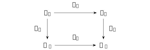
The horizontal maps select a sector; the right map removes one free coordinate within it. The algebra factors \(k\times k\), the full rank-two sectors, and the retained rank-one sectors are different levels of decomposition.
Remark 11.4. Support parity, group degree and sign sectors [fdip-003P]AGENTDRAFTED
- October 29, 2026
Remark 11.4. Support parity, group degree and sign sectors [fdip-003P]AGENTDRAFTED
- October 29, 2026
For the four-cycle over a nonzero commutative ring with invertible two, three decompositions record different structures. The support grading separates fields supported on \(\{0,2\}\) and \(\{1,3\}\). The one-step shift \(Tf(i)=f(i+1)\) exchanges these supports, so it is odd, whereas \(P=T^2\) and \(E_\pm =h(I\pm P)\) preserve them and are even. A single half-turn sign sector contains both \(b_{\varepsilon ,0}=\delta _0+\varepsilon \delta _2\) and \(b_{\varepsilon ,1}=\delta _1+\varepsilon \delta _3\), which have different support parities. A minus eigenvalue does not mean odd support.
The canonical group grading of \(k[C_2]\) has components \(k\,1\) of degree \(1_G\) and \(k\,g\) of degree \(r\). Their multiplication follows the group law, in particular \(g^2=1\). Over a ring these are rank-one free summands. The representation sends \(g\) to support-even \(P\); it therefore does not preserve these particular gradings under \(r\mapsto 1\in \mathbb Z/2\mathbb Z\). The projector ideals are different again: \(e_-^2=e_-\ne 0\), while an odd homogeneous component would have its square in the even component. The direct product, the group grading and the support grading cannot be interchanged. These are the distinct splitting levels applied to the concrete action.
The ordinary adjoint uses the counting pairing \(b(f,u)=\sum _i f_i u_i\), with identity coefficient involution. Delta vectors recover all coefficients, so the pairing is perfect. Reindexing a finite sum shows that every permutation action is an isometry, hence \[b(\rho (\sigma )f,u)=b(f,\rho (\sigma ^{-1})u).\] Uniqueness of the ordinary adjoint gives \(\rho (\sigma )^\dagger =\rho (\sigma ^{-1})\); in particular \(T^\dagger =T^{-1}\) and \(P^\dagger =P\). There is no complex conjugation or Koszul sign in this calculation.
The corresponding ordinary group-algebra operation is \[\left (\sum _g a_g[g]\right )^*=\sum _g a_g[g^{-1}].\] It is \(k\)-linear, fixes scalars, squares to the identity and reverses products, since \((gh)^{-1}=h^{-1}g^{-1}\) and all sums are finite. For an isometric representation with a perfect pairing, taking the adjoint of its finite linear extension therefore gives \(\widehat \rho (z^*)=\widehat \rho (z)^\dagger \). The isometry premise matters: the infinite cyclic group acting on \(\mathbb R\) by multiplication by \(2\) has adjoint \(2\) and inverse \(1/2\), so this identity fails for that representation. The counting action satisfies the premise.
The group basis and inversion are as in [sengupta2010representations, Sections 3.1-3.2, pp. 39-41]; the grading and adjoint comparisons above are direct calculations. The shift calculation supplies the support-degree and adjoint identities. Clifford parity of a quadratic quotient is a further structure; these ordinary formulas introduce neither a graded star nor a Hermitian extension.
Theorem 11.5. The real Gaussian law is a product over orthogonal sectors [fdip-000M]AGENTDRAFTED
- October 17, 2026
Theorem 11.5. The real Gaussian law is a product over orthogonal sectors [fdip-000M]AGENTDRAFTED
- October 17, 2026
Let \(H\) be a finite-dimensional real inner-product space, \(P:H\to H\) an orthogonal involution, and \(Q:H\to H\) a positive self-adjoint precision with \(QP=PQ\). Put \(H_\varepsilon =\ker (P-\varepsilon I)\) and \(E_\varepsilon =(I+\varepsilon P)/2\). Use induced Euclidean volumes on the uncompleted Borel sigma-algebras. The restrictions \(Q_\varepsilon =Q|_{H_\varepsilon }\) are positive self-adjoint. For their Gaussian laws, \[\begin {aligned} D:H&\longrightarrow H_+\times H_-,\\ z&\longmapsto (E_+z,E_-z),\\ D_*\mu _Q&=\mu _{Q_+}\otimes \mu _{Q_-},\qquad Z_Q=Z_{Q_+}Z_{Q_-}. \end {aligned}\] Thus the sector-valued random variables \(E_+,E_-\) are independent with the indicated marginal laws. The four-cycle recovery computes both blocks, their normalizers and their retained scalar laws explicitly.
Proof.
- October 17, 2026
Proof.
- October 17, 2026
The module projector identities give the direct sum. For \(u\in H_+\), \(v\in H_-\), orthogonality of \(P\) gives \(\langle u,v\rangle =\langle Pu,Pv\rangle =-\langle u,v\rangle \), so \(\langle u,v\rangle =0\). Addition \(J:H_+\times H_-\to H\), \(J(u,v)=u+v\), is therefore an isometric linear isomorphism with inverse \(D\). Commutation gives \(PQu=QPu=\varepsilon Qu\) for \(u\in H_\varepsilon \); hence \(Q\) preserves each sector. Restricting its pairing identity and testing nonzero sector vectors proves self-adjointness and positivity of \(Q_\varepsilon \).
Concatenating orthonormal bases of \(H_+,H_-\) gives an orthonormal basis of \(H\). Coordinate product Lebesgue measure, transported by these charts, therefore proves \[J_*(\lambda _+\otimes \lambda _-)=\lambda _H,\qquad D_*\lambda _H=\lambda _+\otimes \lambda _-.\] This is precisely orthogonal product volume. Finite-dimensional spaces have countable bases, so the product Borel sigma-algebra is the Borel sigma-algebra of the product. Bounded coordinate cubes exhaust each space, proving sigma-finiteness. A zero-dimensional sector has unit mass on its sole point.
Orthogonality and preservation of sectors give the action identity \[\langle u+v,Q(u+v)\rangle =\langle u,Q_+u\rangle +\langle v,Q_-v\rangle .\] For \(w_Q(z)=e^{-\langle z,Qz\rangle/2}\), this says \(w_Q(J(u,v))=w_{Q_+}(u)w_{Q_-}(v)\). The positive normalizer theorem applies separately to all three positive self-adjoint maps: \[Z_R=\frac {(2\pi )^{\dim U/2}}{\sqrt {\det R}}\in (0,\infty ) \quad (R=Q,Q_+,Q_-\text { on its space }U).\] Its proof uses positive eigenvalues, the scalar Gaussian integral and nonnegative Tonelli, without presupposing this product law. Empty determinants and normalizers are one. Applying Tonelli with the volume and weight identities just proved gives \(Z_Q=Z_{Q_+}Z_{Q_-}\).
For Borel sets \(A_+\subseteq H_+\), \(A_-\subseteq H_-\), all the following integrands are nonnegative measurable functions: \[\begin {aligned} (D_*\mu _Q)(A_+\times A_-) &=\frac {1}{Z_{Q_+}Z_{Q_-}}\\ &\quad \cdot \int _{A_+\times A_-}w_{Q_+}(u)w_{Q_-}(v) \,d(\lambda _+\otimes \lambda _-)(u,v)\\ &=\mu _{Q_+}(A_+)\mu _{Q_-}(A_-). \end {aligned}\] Rectangles form a pi-system containing the whole product and generating its Borel sigma-algebra. The pi-lambda uniqueness theorem for finite measures identifies the two probability measures everywhere. Their coordinate marginals and the displayed rectangle equation are exactly independence of \(E_+,E_-\). The argument also covers a zero sector, whose law is deterministic. Algebraic splitting alone would not have supplied this probability identity.
For the actual polynomial function algebras, write \(\omega _R(p)=\int p\,d\mu _R\). Then \[\omega _Q\bigl ((p_+\circ E_+)(p_-\circ E_-)\bigr ) =\omega _{Q_+}(p_+)\omega _{Q_-}(p_-).\] Indeed linear precomposition takes polynomial generators to polynomial generators. Every polynomial, product and square has finite absolute Gaussian integral by Proposition 7.11, applied on the full space and on each sector. Tonelli applied first to the absolute product therefore justifies signed Fubini, which gives the formula from the product law. These are real polynomial states: they are linear, normalized and nonnegative on \(p^2\), with the identity star. No algebra structure on all integrable functions, or state on \(\operatorname {End}(H)\), is being used.
[friedli2017statistical, Proposition B.55, p. 505] uses covariance as its positive parameter. In an orthonormal chart, set \(\Sigma =Q^{-1}\). Its eigenvalues are positive, \(\Sigma ^{-1}=Q\) and \(\det \Sigma =(\det Q)^{-1}\), so its normalized density is exactly \(Z_Q^{-1}w_Q\). The inverse-precision covariance theorem identifies \(\Sigma \) as the covariance. The product proof above uses densities, not an inference from zero covariance for an unspecified law.
Mathlib's OrthonormalBasis.measurePreserving_repr
supports passage to orthonormal coordinates. Index coordinates by the
disjoint union of orthonormal bases of \(H_+\) and \(H_-\). Then
\(\Sigma =\operatorname {diag}(Q_+^{-1},Q_-^{-1})\) is positive
definite, hence positive semidefinite, with zero cross block and mean
zero. After the density identification, TauCeti's
TauCeti.Probability.indepFun_sumEquivProd_multivariateGaussian_iff
gives the corresponding coordinate independence. It concerns this
Gaussian covariance, not an arbitrary algebraic splitting or Schur
fiber integral.
The integration convention is [tao2011measure, Theorem 1.7.15, pp. 200-201, preliminary version]. All probability assertions here are finite-dimensional and real, with strictly positive precision and specified volume. They supply no Lebesgue probability over a general coefficient ring; a singular precision needs a separately specified constrained space and law.
Proposition 11.6. Restricting a split Schur map to sign sectors [fdip-003Q]AGENTDRAFTED
- October 29, 2026
Proposition 11.6. Restricting a split Schur map to sign sectors [fdip-003Q]AGENTDRAFTED
- October 29, 2026
Let \(k\) be a commutative unital ring with invertible two and \(H=X\oplus Y\). Let \(P=P_X\oplus P_Y\), where \(P_X^2=I_X\), \(P_Y^2=I_Y\), and let \(Q:H\to H\) commute with \(P\). Write the typed split components as \[\begin {aligned} A&:X\to X,&B&:Y\to X,\\ E&:X\to Y,&C&:Y\to Y,\\ Q(x,y)&=(Ax+By,Ex+Cy). \end {aligned}\] If \(C\) is invertible, the split Schur map \(S=A-BC^{-1}E\) preserves both sign sectors of \(P_X\), and \[S|_{X_\varepsilon } =A_\varepsilon -B_\varepsilon C_\varepsilon ^{-1}E_\varepsilon .\] Here \(X_\varepsilon =\ker (P_X-\varepsilon I)\), \(Y_\varepsilon =\ker (P_Y-\varepsilon I)\), and each subscript means restriction to the indicated source and target sectors.
Proof.
- October 29, 2026
Proof.
- October 29, 2026
Evaluate \(QP=PQ\) on \((x,0)\) and \((0,y)\) and project to both summands. This gives \[\begin {aligned} AP_X&=P_XA,&BP_Y&=P_XB,\\ EP_X&=P_YE,&CP_Y&=P_YC. \end {aligned}\] Multiplying the last identity on both sides by the inverse of \(C\) gives \(C^{-1}P_Y=P_YC^{-1}\). Each of these identities proves that its map takes sign-\(\varepsilon \) vectors to sign-\(\varepsilon \) vectors. In particular \(C_\varepsilon \) is invertible, with inverse \(C^{-1}|_{Y_\varepsilon }\), since the two inverse equations restrict to the sector. Finally \[\begin {aligned} SP_X&=AP_X-BC^{-1}EP_X\\ &=P_XA-BP_YC^{-1}E=P_XS. \end {aligned}\] Restricting the actual composite \(BC^{-1}E:X\to X\) now gives exactly the asserted formula, with no interchange of differently typed factors.
This is the sign-sector specialization of Schur transport, using the module projectors. Its block convention agrees with [boyd2004convex, Appendix A.5.5, pp. 650-651] after exchanging the source's first pivot to \(C\). The proof here is over modules; no pairing, self-adjointness, stationary field or probability law has been assumed. If the prescribed splitting is not preserved by \(P\), the required \(P_X,P_Y\) and these restrictions are not supplied.
Theorem 11.7. Gaussian marginalization commutes with sector decomposition [fdip-003R]AGENTDRAFTED
- October 29, 2026
Theorem 11.7. Gaussian marginalization commutes with sector decomposition [fdip-003R]AGENTDRAFTED
- October 29, 2026
Let \(H=X\mathbin \perp Y\) be a finite-dimensional real orthogonal sum, \(P=P_X\oplus P_Y\) an orthogonal involution, and \(Q\) a positive self-adjoint precision commuting with \(P\). Use induced Euclidean volumes and Borel Gaussian laws. For \(Q(x,y)=(Ax+By,B^\dagger x+Cy)\), put \(S=A-BC^{-1}B^\dagger \). The sign sectors are \(H_\varepsilon =X_\varepsilon \mathbin \perp Y_\varepsilon \). Let \(\pi (x,y)=x\) and let \(\pi _\varepsilon \) be its sector restriction. The typed restriction identity gives \[S_\varepsilon :=S|_{X_\varepsilon } =A_\varepsilon -B_\varepsilon C_\varepsilon ^{-1} B_\varepsilon ^\dagger .\] Then the following square commutes both for maps and for their pushforwards of the Gaussian laws:
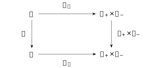
Here \(D_H(z)=(E_+z,E_-z)\) and \(D_X(x)=(F_+x,F_-x)\) are the orthogonal sector decompositions. The full retained law is \(\pi _*\mu _Q=\mu _S\); both routes give \(\mu _{S_+}\otimes \mu _{S_-}\) on \(X_+\times X_-\).
Proof.
- October 29, 2026
Proof.
- October 29, 2026
Testing positivity on \((0,y)\) makes \(C\) positive and invertible. Its inverse is self-adjoint by adjointing both inverse equations, so \(S\) is self-adjoint. With \(K=C^{-1}B^\dagger \), expansion gives \[\langle (x,y),Q(x,y)\rangle =\langle x,Sx\rangle +\langle y+Kx,C(y+Kx)\rangle .\] The two cross terms sum to \(2\langle x,By\rangle \); the last \(K\)-term cancels the subtraction in \(S\). Testing on \((x,-Kx)\) proves \(S>0\). Thus the hypotheses of positive Gaussian elimination hold. For every fixed \(x\), translation by \(Kx\) preserves induced volume, giving the pointwise fiber identity \[\int _Y e^{-\langle (x,y),Q(x,y)\rangle/2}\,d\lambda _Y(y) =Z_C e^{-\langle x,Sx\rangle/2}.\] The normalizer is \(Z_C=(2\pi )^{\dim Y/2}/\sqrt {\det C}\). Nonnegative Tonelli gives \(Z_Q=Z_CZ_S\), and inserting a Borel indicator of \(x\) then dividing proves \(\pi _*\mu _Q=\mu _S\). This is the retained marginal theorem, with its actual volume and positive finite normalizers.
The restricted \(Q_\varepsilon ,C_\varepsilon ,S_\varepsilon \) are positive self-adjoint. Applying the same fiber identity within \(H_\varepsilon \) gives, for every \(x_\varepsilon \), \[\begin {aligned} &\int _{Y_\varepsilon } e^{-\langle (x_\varepsilon ,y),Q_\varepsilon (x_\varepsilon ,y)\rangle/2} \,d\lambda _{Y_\varepsilon }(y)\\ &\qquad =Z_{C_\varepsilon } e^{-\langle x_\varepsilon ,S_\varepsilon x_\varepsilon \rangle/2}. \end {aligned}\] Hence \((\pi _\varepsilon )_*\mu _{Q_\varepsilon }=\mu _{S_\varepsilon }\). The orthogonal product theorem, applied to \(Q,C,S\), gives their product laws and \(Z_C=Z_{C_+}Z_{C_-}\). No scalar factor is discarded before normalization.
Since \(\pi P=P_X\pi \), the projector formulas imply \(\pi E_\varepsilon =F_\varepsilon \pi \), proving the map square. Pushforwards compose by inverse images. The upper route first gives \(\mu _{Q_+}\otimes \mu _{Q_-}\). Its pushforward by \(\pi _+\times \pi _-\) agrees with \(\mu _{S_+}\otimes \mu _{S_-}\) on every Borel rectangle, using the sector marginal identities, and therefore everywhere by uniqueness of probability measures on the rectangle-generated Borel sigma-algebra. The lower route first gives \(\mu _S\); its sector decomposition gives the same product.
Pullback on the polynomial function algebras reverses all 4 arrows. For every polynomial \(f\) on \(X_+\times X_-\), the commuting map square gives \[f\circ D_X\circ \pi =f\circ (\pi _+\times \pi _-)\circ D_H.\] Precomposition by each linear map is a unital algebra homomorphism, as in polynomial transport. For a polynomial \(p\in \operatorname {Pol}(X)\), nonnegative integration first gives \(\int |p\circ \pi |\,d\mu _Q=\int |p|\,d\mu _S\); absolute Gaussian moments make both sides finite for polynomials. Subtraction of positive and negative parts then gives \(\omega _S=\omega _Q\circ \pi ^*\) and the corresponding equalities on every side of the square. This is equality of normalized polynomial functionals, in addition to maps and probability laws.
The specified conditional kernel at eliminated field zero instead has precision \(A\); it need not equal the marginal of precision \(S\). If \(B=0\), then \(S=A\), so equality can occur. The coupled cycle gives a concrete difference. A nonstable retained set does not supply this square: for retention \(\{0,1\}\), \(\pi \delta _2=0\) but \(\pi P\delta _2=\delta _0\). A singular eliminated direction can have infinite fiber integral, as for \(Q(x,y)=(x,0)\) on \(\mathbb R^2\). A pseudoinverse does not make that integral finite. The massless cycle has a constant zero mode and requires a separately specified constrained law.
The Schur convention is [boyd2004convex, Appendix A.5.5, pp. 650-651], with the pivot exchanged to \(C\). The Gaussian density convention is [friedli2017statistical, Proposition B.55, p. 505], where covariance is \(\Sigma =Q^{-1}\). The sector square is the direct combination proved above; the formalization references discussed with the retained marginal theorem support Gaussian images and signed Fubini with their stated hypotheses, not the pointwise fiber constants.
Example 11.8. The complete sector law of the alternating four-cycle [fdip-003S]AGENTDRAFTED
- October 29, 2026
Example 11.8. The complete sector law of the alternating four-cycle [fdip-003S]AGENTDRAFTED
- October 29, 2026
For the alternating four-cycle with \(t,m>0\), the two real half-turn sectors are independent under the Gaussian law. Their precision and covariance blocks vary with \(t,m\), although the action and its projectors do not. Put \(a=m^2\) and \(s=1+t+a\). The counting quadratic form is \[\begin {aligned} \langle \phi ,Q\phi \rangle &=(\phi _1-\phi _0)^2+t(\phi _2-\phi _1)^2\\ &\quad +(\phi _3-\phi _2)^2+t(\phi _0-\phi _3)^2 +a\sum _i\phi _i^2. \end {aligned}\] It is strictly positive for nonzero \(\phi \), since \(a>0\). The weighted incidence construction is self-adjoint, and the half-turn reindexes the 4 edge terms without changing their weights. Thus \(QP=PQ\), as required by the intrinsic product law. In vertex order \((0,1,2,3)\), the massive precision is \[Q=\begin {pmatrix} s&-1&0&-t\\-1&s&-t&0\\0&-t&s&-1\\-t&0&-1&s \end {pmatrix}.\] Use the orthonormal vectors \[\begin {aligned} v_{\varepsilon ,0}&=(\delta _0+\varepsilon \delta _2)/\sqrt 2,\\ v_{\varepsilon ,1}&=(\delta _1+\varepsilon \delta _3)/\sqrt 2, \qquad \varepsilon \in \{1,-1\}. \end {aligned}\] Write \(\phi =\sum _\varepsilon (x_\varepsilon v_{\varepsilon ,0}+y_\varepsilon v_{\varepsilon ,1})\) and \(z_\varepsilon =(x_\varepsilon ,y_\varepsilon )\). These are normalized sector coordinates, rather than the coefficients in the unnormalized free bases of Definition 11.3. In particular \[\begin {aligned} \phi _0&=(x_++x_-)/\sqrt 2,&\phi _2&=(x_+-x_-)/\sqrt 2,\\ \phi _1&=(y_++y_-)/\sqrt 2,&\phi _3&=(y_+-y_-)/\sqrt 2. \end {aligned}\]
In the order \((v_{+,0},v_{+,1},v_{-,0},v_{-,1})\), the precision is \(\operatorname {diag}(Q_+,Q_-)\) and its inverse is \(\operatorname {diag}(G_+,G_-)\), where \[\begin {aligned} Q_+&=\begin {pmatrix}s&-(1+t)\\-(1+t)&s\end {pmatrix},\\ Q_-&=\begin {pmatrix}s&t-1\\t-1&s\end {pmatrix},\\ G_+&=\tfrac 1{a(a+2+2t)} \begin {pmatrix}s&1+t\\1+t&s\end {pmatrix},\\ G_-&=\tfrac 1{(a+2)(a+2t)} \begin {pmatrix}s&1-t\\1-t&s\end {pmatrix}. \end {aligned}\] The covariance in these coordinates is given by the displayed inverse blocks. If \(T\phi =(z_+,z_-)\), then \[T_*\mu _Q=\mu _{Q_+}\otimes \mu _{Q_-}.\] The product on the right is the product probability measure. In particular the sector random vectors \(z_+,z_-\) are independent.
[friedli2017statistical, Proposition B.55, p. 505] gives the Gaussian covariance and coordinate-change convention. The positive Gaussian normalization and inverse-precision covariance apply to each block. The product assertion follows from the explicit density calculation below, rather than from the algebraic direct sum alone.
Proof.
- October 29, 2026
Proof.
- October 29, 2026
Each unnormalized vector has squared norm two, and the pairings between distinct vectors are zero. Thus the basis matrix \(O\) with the displayed columns is orthogonal, \(T=O^T\), and \(|\det O|=1\). Applying \(Q\) gives \[\begin {aligned} Qv_{+,0}&=sv_{+,0}-(1+t)v_{+,1},\\ Qv_{+,1}&=-(1+t)v_{+,0}+sv_{+,1},\\ Qv_{-,0}&=sv_{-,0}+(t-1)v_{-,1},\\ Qv_{-,1}&=(t-1)v_{-,0}+sv_{-,1}. \end {aligned}\] These are precisely the two asserted blocks. Their sum and difference vectors have eigenvalues \[\begin {aligned} Q_+&:\quad a,\ a+2+2t,\\ Q_-&:\quad a+2t,\ a+2. \end {aligned}\] They are all positive. Multiplication by the displayed \(G_\pm \) gives the identity: the diagonal numerators are respectively \(s^2-(1+t)^2=a(a+2+2t)\) and \(s^2-(t-1)^2=(a+2)(a+2t)\), and the off-diagonal numerators vanish. This proves the inverse formulas.
The orthogonal change of variables preserves coordinate Lebesgue measure and writes the Euclidean action as \[\mathcal A(\phi )=\tfrac 12 z_+^TQ_+z_+ +\tfrac 12 z_-^TQ_-z_-.\] Each factor has a finite positive normalizer \[Z_\pm =\frac {2\pi }{\sqrt {\det Q_\pm }}.\] Tonelli's theorem applied to the nonnegative density gives \(Z_Q=Z_+Z_-\). Division by this product yields the product of the two normalized densities. Integrating over every Borel rectangle \(A_+\times A_-\) gives \[\begin {aligned} &\mu _Q\{z_+\in A_+,\ z_-\in A_-\}\\ &\qquad =\mu _{Q_+}(A_+)\mu _{Q_-}(A_-). \end {aligned}\] Rectangles generate the product Borel sigma-algebra, so uniqueness of probability measures identifies the product law and proves independence. In particular it does not assume that zero covariance alone implies independence. Polynomial moments are integrable by Proposition 7.11.
Writing \[\begin {aligned} d_+&=a(a+2+2t),&d_-&=(a+2)(a+2t),\\ \Delta &=d_+d_-=a(a+2)(a+2t)(a+2+2t)>0, \end {aligned}\] the full normalizer is \(Z_Q=4\pi ^2/\sqrt \Delta \).
Retain \(R=(0,2)\). Its orthonormal sector vectors are \[w_\varepsilon =(\delta _0^R+\varepsilon \delta _2^R)/\sqrt 2.\] The projection satisfies \[\begin {aligned} \pi _Rv_{\varepsilon ,0}&=w_\varepsilon ,\\ \pi _Rv_{\varepsilon ,1}&=0. \end {aligned}\] Thus the retained sector coordinates are exactly \(x_+,x_-\), with no additional factor of \(\sqrt 2\). In these coordinates, the retained precision has positive scalar blocks \[\begin {aligned} \sigma _+&=s-\frac {(1+t)^2}{s} =\frac {a(a+2+2t)}s,\\ \sigma _-&=s-\frac {(t-1)^2}{s} =\frac {(a+2)(a+2t)}s. \end {aligned}\] The retained coordinates are independent centered Gaussians with variances \(\sigma _+^{-1},\sigma _-^{-1}\). Decomposing into sectors and taking this marginal therefore give the same law in either order, as in the map and measure square.
Proof.
- October 29, 2026
Proof.
- October 29, 2026
A sector has precision \(\begin {pmatrix}s&c\\c&s\end {pmatrix}\), with \(c=-(1+t)\) or \(c=t-1\). Complete the square: \[\begin {aligned} sx^2+2cxy+sy^2 &=s(y+cx/s)^2\\ &{}+(s-c^2/s)x^2. \end {aligned}\] The scalar Gaussian integral gives \[\begin {aligned} &\int _{\mathbb R} e^{-(sx^2+2cxy+sy^2)/2}\,dy\\ &\qquad =\sqrt {\frac {2\pi }{s}} e^{-(s-c^2/s)x^2/2}. \end {aligned}\] Each eliminated sector coordinate contributes \(\sqrt {2\pi/s}\); the two factors multiply to \(2\pi/s\). This is exactly the factor for the original eliminated block \(C=sI_2\) in Example 9.5. The retained orthogonal change of coordinates also has absolute determinant one. Normalizing the two scalar densities proves the claimed retained product law.
Equivalently, in retained/eliminated vertex order \(X=(0,2)\), \(Y=(1,3)\), the typed arrays are \[A=C=sI_2,\qquad B=E^T=-\begin {pmatrix}1&t\\t&1\end {pmatrix}.\] Thus \(BC^{-1}E=s^{-1}\begin {pmatrix}1+t^2&2t\\2t&1+t^2\end {pmatrix}\), and the effective precision in vertex coordinates is \[\begin {aligned} S&=\begin {pmatrix}\alpha &-\beta \\-\beta &\alpha \end {pmatrix},\\ \alpha &=s-\frac {1+t^2}{s},\qquad \beta =\frac {2t}{s}. \end {aligned}\] It acts on \(w_+\) by \(\alpha -\beta =\sigma _+\), and on \(w_-\) by \(\alpha +\beta =\sigma _-\). Thus each sector's Schur complement agrees with the corresponding block of \(S\).
Direct multiplication also gives \[\begin {aligned} S^{-1}&=\frac {1}{\alpha ^2-\beta ^2} \begin {pmatrix}\alpha &\beta \\\beta &\alpha \end {pmatrix},\\ \alpha ^2-\beta ^2&=\sigma _+\sigma _-=\Delta/s^2>0,\\ Z_S&=\frac {2\pi }{\sqrt {\sigma _+\sigma _-}} =\frac {2\pi s}{\sqrt \Delta }. \end {aligned}\] The full eliminated factor \(2\pi/s\) times \(Z_S\) is exactly \(Z_Q\); both the pointwise fiber constants and the normalized law agree.
See [boyd2004convex, Appendix A.5.5, pp. 650-651] for the general block formula. Restricting \(Q\) to a full sector still leaves two coordinates. Integrating out its second coordinate takes the Schur complement computed above.
Transforming the retained coordinates back gives \[\begin {aligned} \operatorname {Var}(\phi _0) =\operatorname {Var}(\phi _2) &=\tfrac 12(\sigma _+^{-1}+\sigma _-^{-1}),\\ \langle \phi _0\phi _2\rangle _Q &=\tfrac 12(\sigma _+^{-1}-\sigma _-^{-1}). \end {aligned}\] For \(m=t=1\), the sector blocks and their inverses are \[\begin {aligned} Q_+&=\begin {pmatrix}3&-2\\-2&3\end {pmatrix},&Q_-&=3I_2,\\ G_+&=\tfrac 15\begin {pmatrix}3&2\\2&3\end {pmatrix},&G_-&=I_2/3. \end {aligned}\] Hence \(\sigma _+=5/3\), \(\sigma _-=3\); the retained variance is \(7/15\) and the cross covariance is \(2/15\). Directly, \[\begin {aligned} S&=\tfrac 13\begin {pmatrix}7&-2\\-2&7\end {pmatrix},& S^{-1}&=\tfrac 1{15}\begin {pmatrix}7&2\\2&7\end {pmatrix},\\ Z_Q&=\frac {4\pi ^2}{3\sqrt 5},&Z_S&=\frac {2\pi }{\sqrt 5}. \end {aligned}\] The eliminated factor is \(2\pi/3\). The specified conditional kernel at eliminated field zero instead gives precision \(A=3I_2\) and covariance \(I_2/3\), whose zero cross covariance differs from \(2/15\). For \(m=1,t=2\), \[\begin {aligned} Q_+&=\begin {pmatrix}4&-3\\-3&4\end {pmatrix},\\ Q_-&=\begin {pmatrix}4&1\\1&4\end {pmatrix},\\ G_+&=\tfrac 17\begin {pmatrix}4&3\\3&4\end {pmatrix},\\ G_-&=\tfrac 1{15}\begin {pmatrix}4&-1\\-1&4\end {pmatrix}. \end {aligned}\] Now \(\sigma _+=7/4\), \(\sigma _-=15/4\); the retained variance is \(44/105\) and the cross covariance is \(16/105\). Here \[\begin {aligned} S&=\begin {pmatrix}11/4&-1\\-1&11/4\end {pmatrix},\\ S^{-1}&=\tfrac 1{105}\begin {pmatrix}44&16\\16&44\end {pmatrix},\\ Z_Q&=\frac {4\pi ^2}{\sqrt {105}},&Z_S&=\frac {8\pi }{\sqrt {105}}. \end {aligned}\] The eliminated factor is \(\pi/2\). Both examples have the same \(P,J,E_\pm ,F_\pm \), but different covariance matrices and hence different Gaussian states: their polynomial functionals differ on \(\phi _0\phi _2\).
The half-turn commutant explains why these two-dimensional precision blocks may mix coordinates while respecting the same symmetry.
Mathlib's OrthonormalBasis.measurePreserving_repr
supplies the volume-preserving passage to orthonormal coordinates.
TauCeti's
TauCeti.Probability.indepFun_sumEquivProd_multivariateGaussian_iff
characterizes independence of complementary coordinate blocks by
vanishing cross covariance. Index each sector by \(\{0,1\}\) and
the full coordinates by the disjoint union of these sets. Take mean
zero and covariance \(\Sigma =\operatorname {diag}(G_+,G_-)\).
The positive eigenvalues above make \(\Sigma \) positive definite,
hence positive semidefinite, and its cross block is zero.
After identifying the normalized sector density with this Gaussian
law, the theorem gives independence. The formalization references discussed
with the inverse-precision covariance theorem use
\(G_\pm =Q_\pm ^{-1}\) as their parameters. The concrete matrices,
density identification and sectorwise Schur calculation are supplied
by the proofs above.
Proposition 11.9. The half-turn commutant permits mixing within a sector [fdip-003T]AGENTDRAFTED
- October 29, 2026
Proposition 11.9. The half-turn commutant permits mixing within a sector [fdip-003T]AGENTDRAFTED
- October 29, 2026
For the real half-turn, define its commutant by \(\operatorname {Comm}(P)=\{R\in \operatorname {End}_{\mathbb R}(V):RP=PR\}\). Restriction to the two sectors gives an algebra isomorphism \[\operatorname {Comm}(P) \cong \operatorname {End}(V_+)\times \operatorname {End}(V_-) \cong M_2(\mathbb R)\times M_2(\mathbb R).\] If \(R\) commutes with \(P\) and \(Pv=\varepsilon v\), then \(PRv=RPv=\varepsilon Rv\), so it preserves each sector. Conversely, a map preserving both sectors obeys \(PR(v_++v_-)=Rv_+-Rv_-=RP(v_++v_-)\). The inverse to restriction acts separately on the unique sector components; composition and the unit are componentwise. The explicit bases identify each endomorphism algebra with \(M_2(\mathbb R)\).
In sector coordinates \(P=\operatorname {diag}(I_2,-I_2)\). For \(R=\begin {pmatrix}A&B\\C&D\end {pmatrix}\), direct comparison gives \[RP=PR\quad \Longleftrightarrow \quad 2B=2C=0 \quad \Longleftrightarrow \quad B=C=0.\] The group-algebra image is the strictly smaller algebra \[\{\operatorname {diag}(xI_2,yI_2):x,y\in \mathbb R\}.\] Indeed \(aI+bP\) has \(x=a+b\), \(y=a-b\), and every pair is obtained from \(a=(x+y)/2\), \(b=(x-y)/2\). The map swapping \(b_{+,0},b_{+,1}\) and vanishing on \(V_-\) belongs to the commutant but is not scalar on \(V_+\), proving strict containment.
Each sign occurs twice, so an operator commuting with \(P\) may mix the two vectors in either sector. Symmetry therefore does not force \(Q_\pm \) to be scalar; the cycle precision blocks exhibit the freedom explicitly. The group-algebra/module convention comes from [sengupta2010representations, Sections 3.1-3.2, pp. 39-41]; the commutant calculation is direct. The interpretation boundary remains: this finite algebra calculation selects no continuous gauge group, physical mass spectrum or interaction.
Example 11.10. The half-turn in characteristic two [fdip-000N]AGENTDRAFTED
- October 17, 2026
Example 11.10. The half-turn in characteristic two [fdip-000N]AGENTDRAFTED
- October 17, 2026
The coefficient assumption in the two-sector decomposition is essential. Let \(k\) now be a nonzero commutative ring of characteristic two. Use the same \(C_2\), group-basis element \(g\), coordinate modules \(V_k,W_k\), and maps \(P,J\). The faithful algebra actions still exist, but the algebra is \[k[C_2]\cong k[z]/(z^2),\] and its idempotents are exactly the scalar idempotents of \(k\). In particular, if \(k\) is a field, it has no idempotents other than \(0,1\), so it cannot be isomorphic to \(k\times k\).
The Group Algebra still has its group basis, as in [sengupta2010representations, Sections 3.1-3.2, pp. 39-41]. The character projectors in [sengupta2010representations, Section 4.5, p. 63] require the group order to be invertible in the field. The following calculation identifies what replaces that product when the order is zero in \(k\).
Proof.
- October 17, 2026
Proof.
- October 17, 2026
Put \(\eta =g-1\). Its coefficient at \(g\) is \(1\), so \(\eta \ne 0\); nevertheless \[\eta ^2=g^2-2g+1=0.\] Since \(g=1+\eta \), the pair \(1,\eta \) is a basis: \[c+d\eta =(c-d)+dg,\] so coefficient comparison proves independence as well as spanning. Evaluation at \(\eta \) therefore induces a unital \(k\)-algebra map \[\begin {aligned} \Psi :k[z]/(z^2)&\longrightarrow k[C_2],\\ [f(z)]&\longmapsto f(\eta ). \end {aligned}\] It is well defined because \(\eta ^2=0\). Every polynomial has a unique remainder \(c+dz\) modulo the monic polynomial \(z^2\): write \(f=c+dz+z^2q\), and observe that a multiple of \(z^2\) has zero constant and linear coefficients. Hence the quotient has basis \([1],[z]\), even when \(k\) has zero divisors. The map sends it to the basis \(1,\eta \), so it is bijective, with inverse \(a+bg\mapsto [(a+b)+bz]\). Evaluation and its inverse preserve the unit and scalars. The algebra \(k[z]/(z^2)\) is the algebra of dual numbers over \(k\); its nonzero element \([z]\) has square zero.
If \(c+d\eta \) is idempotent, commutativity and characteristic two give \[(c+d\eta )^2=c^2.\] Comparison in the basis \(1,\eta \) forces \(d=0\) and \(c^2=c\); conversely every such scalar is idempotent. If \(k\) is a field, or more generally has no zero divisors, \(c(c-1)=0\) implies \(c=0\) or \(c=1\). Both are idempotent. In contrast, \((1,0)\) is a nonzero idempotent different from the unit in \(k\times k\). An algebra isomorphism preserves these properties, which rules out the product. The field hypothesis matters: a general characteristic-two ring can already have nontrivial scalar idempotents. For example \(k=\mathbb F_2\times \mathbb F_2\) has 4 scalar idempotents, including \((1,0)\) and \((0,1)\); all 4 remain idempotent in \(k[z]/(z^2)\). Thus the assertion of exactly two idempotents does not extend to every characteristic-two ring, nor does it rule out all product decompositions in that generality.
On the vertex module, the same half-turn still satisfies \(P^2=I\), while \(-1=1\). Its two proposed eigenspaces now coincide: \[\begin {aligned} \ker (P-I)&=\ker (P+I)\\ &=\{(x,y,x,y):x,y\in k\}. \end {aligned}\] Its coordinate basis is \(\delta _0+\delta _2,\delta _1+\delta _3\): coordinates zero and one recover the coefficients. It is free of rank two (dimension two over a field); adding it to itself does not recover the full module, because \(\delta _0\) is not in it. On the retained module, \[\begin {aligned} \ker (J-I)&=\ker (J+I)\\ &=\{(x,x):x\in k\}, \end {aligned}\] whose basis is \(\delta _0^R+\delta _2^R\), with its coefficient recovered at zero. It has free rank one, and dimension one over a field. These equalities follow directly from the coordinate formulas for \(P,J\).
The nonzero nilpotent is visible in the faithful action as well. For \(N=P-I\), \[\begin {aligned} N^2&=P^2-2P+I=0,\\ N\delta _0&=\delta _2-\delta _0\ne 0. \end {aligned}\] The last vector has coefficient \(1\) at coordinate \(2\). Similarly, \(J-I\) is nonzero on \(\delta _0^R\) and has square zero: \((J-I)\delta _0^R=\delta _2^R-\delta _0^R\ne 0\). Both coordinate injectivity proofs for the algebra actions in Definition 11.3 still apply. Thus the nilpotent \(\eta \) has a faithful nonzero action on both modules. The expressions \((I\pm P)/2\) and \((I\pm J)/2\) are undefined because \(2=0\). The action and projection intertwiner survive, but the complementary projectors and eigenspace direct sum do not. This is a change of coefficient ring for the algebra and modules; the real Gaussian law is not being extended to characteristic two.
TauCeti's
MonoidAlgebra.isIdempotentElem_cyclicTwo_iff
proves the idempotent obstruction more generally for a commutative
nonzero ring without zero divisors in which \(2\) is not a unit. A
characteristic-two field meets these hypotheses. The generator is
identified with \(\operatorname {Multiplicative.ofAdd}
(1:\mathbb Z/2\mathbb Z)\) as in Theorem 11.2.
Indeed, if \(a+bg\) is idempotent, coefficient comparison gives
\(a^2+b^2=a\) and \(2ab=b\). Hence \(b(2a-1)=0\).
If \(b\ne 0\), absence of zero divisors gives \(2a=1\), contradicting
the nonunit hypothesis. Therefore \(b=0\) and \(a\in \{0,1\}\).
This argument does not require characteristic two, but does require
absence of zero divisors. The dual-number presentation and the
coordinate nilpotent above are separate characteristic-two calculations.
12. Finite-group symmetry of Gaussian fields [fdip-004R]AGENTDRAFTED
- October 31, 2026
12. Finite-group symmetry of Gaussian fields [fdip-004R]AGENTDRAFTED
- October 31, 2026
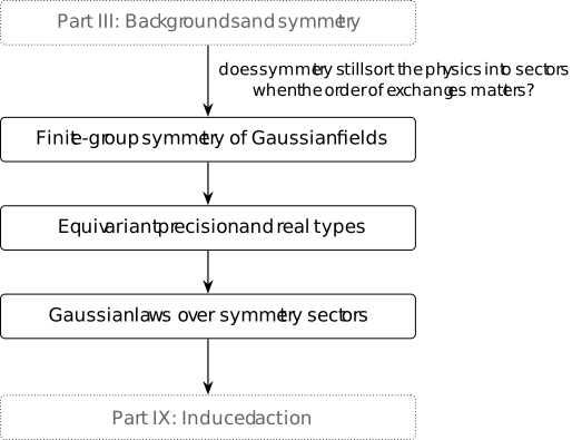
The half-turn splits fields into two sectors that its commuting precision does not mix. Does symmetry still separate the field when the order of exchanges matters? On the uniform cycle, each complex scalar Fourier wave spans a one-dimensional sector labelled by a discrete momentum. Real fields pair the nonexceptional momenta \(k\) and \(-k\) in a two-dimensional sector. For a general finite group, an isotypic sector collects all copies of one irreducible real representation: precision preserves that whole sector but can mix repeated copies within it. Orthogonal projectors recover these sectors from complex characters paired under conjugation. The prerequisites are signed endpoint actions, massive graph precision and the group-algebra extension.
Signed symmetries preserve the quadratic energy even when an edge is reversed. Maschke averaging and the complex central-idempotent formula supply the representation theory; the real projector theorem then gives a complete orthogonal decomposition preserved by precision. The cyclic and dihedral calculations show the resulting subspaces and eigenvalues explicitly.
Definition 12.1. Finite symmetries of a Gaussian background [fdip-004S]AGENTDRAFTED
- October 31, 2026
Definition 12.1. Finite symmetries of a Gaussian background [fdip-004S]AGENTDRAFTED
- October 31, 2026
Fix finite incidence data \((V,E,s,h)\), weights \(w_e>0\), a constant mass \(m>0\), and counting pairings on \(H=\mathbb R^V\) and \(\mathbb R^E\). A finite symmetry of a Gaussian background is a finite group \(G\) with a weight-preserving signed endpoint action \(g\mapsto (p_g,q_g,\varepsilon _g)\) on these data. No retained subset is selected here: in the signed-arrow definition one may take \(R=V\). An additional retained subset would have to be \(G\)-stable. The signs belong to the abstract \(C_2\) of that definition, with \(\sigma (+)=1\) and \(\sigma (-)=-1\). This unpartitioned data does not assert preservation of a nonempty proper retained set as in Definition 10.7.
The vertex and edge representations are \[\begin {aligned} (\rho (g)f)(p_g(v))&=f(v),\\ (J_ga)(q_g(e))&=\sigma (\varepsilon _g(e))a(e). \end {aligned}\] Thus \(\rho (g)f=f\circ p_g^{-1}\); in particular \(\rho (g)\delta _v=\delta _{p_g(v)}\). We call \(H\) with this action the vertex permutation module. With \((df)(e)=f(h(e))-f(s(e))\), the endpoint equations give \(d\rho (g)=J_gd\). The sign cocycle gives \(\rho (gk)=\rho (g)\rho (k)\) and \(J_{gk}=J_gJ_k\). These conventions are the real specialization of Definition 10.1, whose proof includes loops and parallel edge labels.
Write \(W=\operatorname {diag}(w_e)\) and \(Q=d^*Wd+m^2I\) for the massive precision. A reflection may reverse the chosen edge orientations; it is then a signed symmetry, not necessarily a directed relabeling in Definition 10.7. Forgetting those orientations preserves the energy, while still retaining incidence, weights and distinct edge labels. The underlying permutation-representation convention is [milne2025group, Example 7.1(b), p. 101]; the signed extension and its endpoint requirements are proved in Definition 10.1.
Lemma 12.2. Signed symmetries commute with massive precision [fdip-004T]AGENTDRAFTED
- October 31, 2026
Lemma 12.2. Signed symmetries commute with massive precision [fdip-004T]AGENTDRAFTED
- October 31, 2026
For a finite symmetry of a Gaussian background, \(\rho (g)\) and \(J_g\) are orthogonal, \(J_gW=WJ_g\), and \[\rho (g)^*Q\rho (g)=Q,\qquad Q\rho (g)=\rho (g)Q.\] The Green operator \(Q^{-1}\) also commutes with every \(\rho (g)\).
Proof.
- October 31, 2026
Proof.
- October 31, 2026
Reindexing the counting sums gives \[\begin {aligned} \langle \rho (g)f,\rho (g)u\rangle _V&=\langle f,u\rangle _V,\\ \langle J_ga,J_gb\rangle _E&=\langle a,b\rangle _E. \end {aligned}\] The edge signs have square one. Since \(w_{q_g(e)}=w_e\), evaluation at \(q_g(e)\) proves \(WJ_g=J_gW\), and hence \(J_g^*WJ_g=W\). Using the incidence intertwiner, \[\begin {aligned} \rho (g)^*Q\rho (g) &=(d\rho (g))^*W(d\rho (g))+m^2I\\ &=d^*J_g^*WJ_gd+m^2I=Q. \end {aligned}\] Multiply on the left by \(\rho (g)\) to obtain commutation. Multiplication by \(Q^{-1}\) on both sides then proves the inverse claim. Equivalently, each reversed difference changes sign in \(\sum _e w_e(f(h(e))-f(s(e)))^2\) and leaves its square unchanged.
This specializes signed operator transport to positive real data. The incidence convention is [spielman2009effective, Section 2.1, pp. 4-5]; the argument above also covers loops and parallel labels.
Remark 12.3. From the half-turn to a finite group [fdip-004U]AGENTDRAFTED
- October 31, 2026
Remark 12.3. From the half-turn to a finite group [fdip-004U]AGENTDRAFTED
- October 31, 2026
For the four-cycle half-turn, \(G=C_2=\{1,r\}\) and \(\rho (r)=P\). Its two projectors are \((I+P)/2\) and \((I-P)/2\), with the concrete two-dimensional ranges. A larger symmetry group can split these ranges further; a sector for one chosen group is not an intrinsic label independent of that choice.
The group-algebra extension gives \[\widehat \rho :\mathbb R[G]\longrightarrow \operatorname {End}_{\mathbb R}(H), \qquad \widehat \rho \left (\sum _g a_g[g]\right )=\sum _g a_g\rho (g).\] It uses the group algebra and representation/module correspondence. Since every \(\rho (g)\) commutes with \(Q\), so does every \(\widehat \rho (a)\). The action groupoid organizes transported backgrounds, whereas this representation describes a fixed background's symmetry. The character-projector construction in [serre1977linear, Section 2.6, Theorem 8, pp. 21-22] recovers exactly the two half-turn projectors.
Theorem 12.4. Maschke averaging [fgap-001K]
L∃∀NAGENTDRAFTED
Theorem 12.4. Maschke averaging [fgap-001K]
L∃∀NAGENTDRAFTED
Let \(G\) be finite and \(k\) a field in which \(|G|\) is invertible. Every subrepresentation \(W\subseteq V\) has a \(G\)-stable complement. Consequently every finite-dimensional \(k[G]\)-module, and \(k[G]\) itself, is semisimple.
Proof.
Proof.
Choose a \(k\)-linear projection \(P:V\to W\) and average its conjugates: \[ P_G=\frac 1{|G|}\sum _{g\in G}\rho (g)P\rho (g)^{-1}. \] Then \(P_G\) remains the identity on \(W\) and commutes with \(G\). Its kernel is a \(G\)-stable complement. Division by \(|G|\) requires the stated invertibility hypothesis. This is Maschke's theorem as proved in [sengupta2010representations, thm. 3.5.1, pp. 44-46].
Theorem 12.5. primitive central idempotents as block projectors [fgap-001N]
Theorem 12.5. primitive central idempotents as block projectors [fgap-001N]
Over a splitting field of characteristic not dividing \(|G|\), an irreducible character \(\chi \) defines the central element \[ e_\chi =\frac {\chi (1)}{|G|}\sum _{g\in G}\chi (g^{-1})[g]. \] It is a nonzero primitive central idempotent. On a simple module with character \(\psi \), it acts as the identity if \(\psi =\chi \) and as zero otherwise. Distinct \(e_\chi \) are therefore orthogonal block projectors. See [lux2010representations, thm. 2.1.6 and cor. 2.1.7, pp. 88-90]. A constructed family of such projectors does not yield a complete block decomposition until a sum-to-1 statement is also known.
Theorem 12.6. Complete orthogonal real isotypic projectors [fdip-004V]AGENTDRAFTED
- October 31, 2026
Theorem 12.6. Complete orthogonal real isotypic projectors [fdip-004V]AGENTDRAFTED
- October 31, 2026
Let \(G\) be finite and let \(\rho \) be an orthogonal action on a finite-dimensional real inner-product space \(H\). Let \(Q\) be a linear operator commuting with every \(\rho (g)\). Write \(\operatorname {Irr}_{\mathbb C}(G)\) for the irreducible complex characters. For each orbit \(\Xi \) under \(\chi \mapsto \overline \chi \), put \[\begin {aligned} e_\chi &=\frac {\chi (1)}{|G|}\sum _{g\in G}\chi (g^{-1})[g],\\ \epsilon _\Xi &=\sum _{\chi \in \Xi }e_\chi , & P_\Xi &=\widehat \rho (\epsilon _\Xi ). \end {aligned}\] Then \(\epsilon _\Xi \) belongs to \(\mathbb R[G]\), is central, and is fixed by the real involution \([g]^*=[g^{-1}]\). The operators satisfy \[\begin {aligned} P_\Xi ^2&=P_\Xi =P_\Xi ^*,& QP_\Xi &=P_\Xi Q,\\ P_\Xi P_\Upsilon &=0\quad (\Xi \ne \Upsilon ),& \sum _\Xi P_\Xi &=I_H. \end {aligned}\] Thus \(H\) is the orthogonal direct sum of their ranges; a range may be zero. These ranges are its real isotypic sectors: each is the sum of all irreducible real subrepresentations of one isomorphism type. Complexification of a sector is the sum of the complex isotypic components with characters in \(\Xi \).
Proof.
- October 31, 2026
Proof.
- October 31, 2026
Maschke's theorem and the complex central-idempotent formula give central, pairwise orthogonal idempotents \(e_\chi \) acting on the indicated complex components. Coefficient conjugation sends \(e_\chi \) to \(e_{\overline \chi }\), so it fixes \(\epsilon _\Xi \); its coefficients are real. Average a Hermitian inner product on a complex representation over \(G\). Each group operator becomes unitary, whence \(\chi (g^{-1})=\overline {\chi (g)}\). The complex linear extension of \([g]\mapsto [g^{-1}]\) therefore sends \(e_\chi \) to \(e_{\overline \chi }\), and fixes \(\epsilon _\Xi \). This is coefficient conjugation and inversion separately; the latter restricts to the stated real involution.
For completeness, the regular character is \(r_G(g)=|G|\,\delta _{g,1}\) and decomposes as \(r_G=\sum _\chi \chi (1)\chi \) by [serre1977linear, Section 2.4, Proposition 5 and Corollary 1, p. 18]. Consequently \[\begin {aligned} \sum _\chi e_\chi &=\frac 1{|G|}\sum _{g\in G} \left (\sum _\chi \chi (1)\chi (g^{-1})\right )[g]\\ &=\frac 1{|G|}\sum _{g\in G}r_G(g^{-1})[g]=[1]. \end {aligned}\] Grouping by conjugation orbits preserves this sum. Applying \(\widehat \rho \) gives idempotence, mixed-product zero and sum \(I_H\). Orthogonality gives \(\rho (g)^*=\rho (g^{-1})\), so \(\widehat \rho (a^*)=\widehat \rho (a)^*\) for real coefficients. Thus each \(P_\Xi \) is self-adjoint; distinct ranges are perpendicular because \(\langle P_\Xi x,P_\Upsilon y\rangle =\langle x,P_\Xi P_\Upsilon y\rangle =0\). The sum identity gives existence of the decomposition, and applying each projector gives its uniqueness. Commutation with \(Q\) follows by linearity from commutation with every group operator.
To justify the real isotypic terminology, decompose \(H\) into irreducible real subrepresentations by Maschke. On any such \(U\), the real commuting idempotents \(P_\Xi \) have invariant ranges, so exactly one acts as the identity and the rest as zero. Its complexification therefore has constituents in just that orbit. Two real irreducibles assigned to the same orbit share a complex constituent: complex conjugation on each complexification exchanges the constituents indexed by \(\chi \) and \(\overline \chi \). Semisimplicity over \(\mathbb C\) then gives a nonzero complex intertwiner between their complexifications. In real bases, the real and imaginary parts of its matrix are real intertwiners, at least one nonzero. Its kernel and image are invariant, so irreducibility makes it an isomorphism. Conversely an isomorphism commutes with all the character projectors. This proves precisely the asserted grouping.
Serre's [serre1977linear, Section 2.6, Theorem 8, p. 21]
gives the canonical complex components and their projectors; the
real grouping and adjoint argument above are deductions from it.
TauCeti's
TauCeti.Representation.sum_primitiveCentralIdempotent
proves the complex sum-to-one identity for a finite pairwise inequivalent
family of irreducibles whose cardinality equals the number of conjugacy
classes, over an algebraically closed field with invertible group order.
It supports the completeness step, not the real adjoint or graph claims.
Example 12.7. Real Fourier sectors of a cycle [fdip-004W]AGENTDRAFTED
- October 31, 2026
Example 12.7. Real Fourier sectors of a cycle [fdip-004W]AGENTDRAFTED
- October 31, 2026
Let \(n\ge 3\), \(V=E=\mathbb Z/n\mathbb Z\), with edge \(e_v\) from \(v\) to \(v+1\), uniform weight \(w>0\) and mass \(m>0\). The generator \(r\) of \(C_n\) sends \(v\) to \(v+1\) and \(e_v\) to \(e_{v+1}\), with every edge sign positive. Its action on fields is \((\rho (r)f)(v)=f(v-1)\). The cyclic characters in [serre1977linear, Section 5.1, p. 35] and the real projectors yield the following direct calculation.
Set \(\theta _k=2\pi k/n\). The normalized constant vector \(u_0(v)=1/\sqrt n\) spans the trivial sector. For \(1\le k<n/2\), the sector \(H_k\) has orthonormal basis \[c_k(v)=\sqrt {2/n}\cos (\theta _kv),\qquad s_k(v)=\sqrt {2/n}\sin (\theta _kv).\] When \(n\) is even there is also \(u_{n/2}(v)=(-1)^v/\sqrt n\). These give all sectors indexed by \(0\le k\le \lfloor n/2\rfloor \). In the ordered basis \((c_k,s_k)\), the rotation is \[\rho (r)|_{H_k}=\begin {pmatrix} \cos \theta _k&-\sin \theta _k\\ \sin \theta _k&\cos \theta _k \end {pmatrix}.\] For \(0<\theta _k<\pi \) it has no real eigenline, so \(H_k\) is real irreducible. Its complex constituents have characters \(r\mapsto e^{i\theta _k}\) and \(r\mapsto e^{-i\theta _k}\).
Proof.
- October 31, 2026
Proof.
- October 31, 2026
The finite geometric sum \(\sum _{v=0}^{n-1}e^{2\pi i jv/n}\) equals \(n\) when \(n\) divides \(j\) and zero otherwise. Taking real and imaginary parts proves all stated norms and orthogonality. There are \(n\) basis vectors, so they span \(H\). The addition formulas give the displayed rotation. A real rotation through \(0<\theta _k<\pi \) has eigenvalues \(e^{\pm i\theta _k}\), neither real, proving the irreducibility claim.
The precision and each sector eigenvalue are \[\begin {aligned} (Qf)(v)&=(m^2+2w)f(v)-wf(v-1)-wf(v+1),\\ Q|_{H_k}&=q_kI,\\ q_k&=m^2+2w(1-\cos \theta _k). \end {aligned}\] Substitution of each sine, cosine and exceptional one-dimensional mode proves the formula. The orthogonal projector kernels are \[\begin {aligned} P_0(v,u)&=1/n,\\ P_k(v,u)&=\frac 2n\cos (\theta _k(v-u))\quad (0<k<n/2),\\ P_{n/2}(v,u)&=(-1)^{v-u}/n\quad (n\text { even}). \end {aligned}\] They follow by summing the outer products of the displayed orthonormal basis vectors, so their sum is the identity. For \(n=3\), this reads \(P_0=\mathbf 1\mathbf 1^T/3\) and \(P_1=I-P_0\); the eigenvalues are \(m^2\) and \(m^2+3w\), the latter twice. The later circle comparison rescales these same finite modes; no continuum limit is used in this calculation.
Example 12.8. Dihedral symmetry refines the four-cycle sectors [fdip-004X]AGENTDRAFTED
- October 31, 2026
Example 12.8. Dihedral symmetry refines the four-cycle sectors [fdip-004X]AGENTDRAFTED
- October 31, 2026
Take the cycle with \(n=4\), \(w=m=1\). Let \(D_4=\langle r,s:r^4=s^2=1,\ srs=r^{-1}\rangle \), of order 8, act on vertices by \(r(v)=v+1\), \(s(v)=-v\). On the oriented edges \(e_v:v\to v+1\), rotation sends \(e_v\) to \(e_{v+1}\) with positive sign, while reflection sends \(e_v\) to \(e_{-v-1}\) with negative sign. The latter edge runs from \(-v-1\) to \(-v\), the reverse of the transported endpoints. The 4 rotations restore each edge; two reflections restore its label and give positive sign. Reflecting, rotating, then reflecting sends \(e_v\) to \(e_{v-1}\) with two negative signs, hence agrees with the inverse rotation. The vertex maps obey the same relations, so these maps define a signed endpoint action. This uses the dihedral presentation in [serre1977linear, Section 5.3, p. 36]; the edge signs and precision calculation are explicit here.
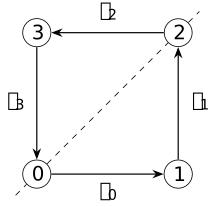
The dashed diagonal is the reflection axis: \(s\) fixes vertices \(0,2\), exchanges \(1,3\), and sends \(e_0\) to \(e_3\) with reversed orientation. All 4 weights and the mass are one.
An orthonormal basis, grouped by real irreducible type, is \[\begin {aligned} u&=(1,1,1,1)/2,&a&=(1,-1,1,-1)/2,\\ c&=(1,0,-1,0)/\sqrt 2,&b&=(0,1,0,-1)/\sqrt 2. \end {aligned}\] The line \(\mathbb Ru\) is trivial. On \(\mathbb Ra\), rotation acts by \(-1\) and reflection by \(+1\); call this the alternating line. On \(K=\operatorname {span}(c,b)\), \[\rho (r)|_K=\begin {pmatrix}0&-1\\1&0\end {pmatrix},\qquad \rho (s)|_K=\begin {pmatrix}1&0\\0&-1\end {pmatrix}.\] There is no real rotation-invariant line, so \(K\) is irreducible. A real matrix commuting with the rotation is \(xI+y\rho (r)\); commuting also with the reflection forces \(y=0\). Thus its commuting algebra is \(\mathbb R I\), the real-type case. The two distinct lines and \(K\) are pairwise nonisomorphic, each occurring once.
Direct substitution in the cycle precision gives \[Qu=u,\qquad Qa=5a,\qquad Qc=3c,\qquad Qb=3b.\] The three orthogonal projectors are \(uu^T\), \(aa^T\), and \(cc^T+bb^T=I-uu^T-aa^T\); their ranges have dimensions \(1,1,2\) and precision eigenvalues \(1,5,3\), respectively. For the subgroup generated by \(r^2\), the positive sector is \(\operatorname {span}(u,a)\) and the negative sector is \(K\). The half-turn calculation therefore has two \(2\times 2\) blocks, whereas the full dihedral action separates its positive block into two lines. Changing the acting group changes the isotypic decomposition without changing this precision.
13. Equivariant precision and real types [fdip-004Y]AGENTDRAFTED
- November 1, 2026
13. Equivariant precision and real types [fdip-004Y]AGENTDRAFTED
- November 1, 2026
A symmetry sector need not have a single precision eigenvalue. Several copies of the same irreducible representation can mix, as the half-turn commutant already shows. The real isotypic projectors separate inequivalent types; within each sector a matrix over the reals, complexes or quaternions records the remaining freedom.
The commutant and positive cone determine the size of these matrices. The Frobenius-Schur indicator then identifies their scalar algebra, with an explicit passage from complex invariant forms to real modules. A twisted prism exhibits a complex multiplicity matrix, and the binary tetrahedral Cayley graph exhibits all three scalar types. Throughout, a Laplacian block becomes a positive precision block only after the specified mass shift.
Theorem 13.1. The real commutant and multiplicity matrices [fdip-004Z]AGENTDRAFTED
- November 1, 2026
Theorem 13.1. The real commutant and multiplicity matrices [fdip-004Z]AGENTDRAFTED
- November 1, 2026
Let a finite group \(G\) act orthogonally on a finite-dimensional real space \(H\). In its isotypic decomposition, write \(H_\Xi \cong W_\Xi ^{\oplus m_\Xi }\), where \(W_\Xi \) is irreducible and \(m_\Xi >0\) is its multiplicity. The commutant consists of all linear maps commuting with \(G\). With multiplication given by composition, put \(D_\Xi =\operatorname {End}_G(W_\Xi )\). Then \[\begin {aligned} D_\Xi &\cong \mathbb R,\ \mathbb C\ \text {or}\ \mathbb H,\\ \operatorname {End}_G(H)&\cong \prod _\Xi M_{m_\Xi }(D_\Xi ). \end {aligned}\] The isomorphism can be chosen to carry adjunction to conjugate transpose. If \(H=\mathbb R^V\) is a vertex permutation representation, the real dimension of \(\operatorname {End}_G(H)\) is the number of orbits of the diagonal action \(g(u,v)=(gu,gv)\) on \(V\times V\). These orbits are called orbitals.
Proof.
- November 1, 2026
Proof.
- November 1, 2026
Maschke's theorem decomposes \(H\) orthogonally into irreducibles. The kernel and image of an intertwiner are invariant. Hence an intertwiner between inequivalent irreducibles is zero, and every nonzero endomorphism of one irreducible is invertible. Thus \(D_\Xi \) is a finite-dimensional associative real division algebra; Frobenius's division-algebra theorem gives the three displayed possibilities. Between \(m_\Xi \) identified copies the intertwiners are precisely matrices of elements of \(D_\Xi \), acting by \((Aw)_i=\sum _j A_{ij}(w_j)\). This proves the algebra statement. The real classification and its representation-theoretic use are [serre1977linear, Section 13.2, pp. 106-109]; compare the real-type distinction.
Adjunction preserves \(D_\Xi \). A self-adjoint element of it has real eigenspaces invariant under \(G\), so irreducibility makes it a real scalar. In particular \(d^*d=cI\) with \(c>0\) for \(d\ne 0\). The resulting positive adjoint on \(\mathbb R\), \(\mathbb C\) or \(\mathbb H\) is the usual conjugation: for an imaginary unit \(j^2=-1\), write \(j+j^*=2aI\) with \(a\in \mathbb R\). Then \(j^*j=2aj+I\) is scalar, forcing \(a=0\). Thus \(j^*=-j\). Identifications between equivalent orthogonal copies can be made isometric by dividing an intertwiner by the positive square root of its scalar \(T^*T\). In those coordinates the block adjoint is conjugate transpose.
For vertex permutations, a matrix \(A\) commutes with every \(\rho (g)\) exactly when \(A_{gu,gv}=A_{u,v}\). Its entries are therefore constant on orbitals. The indicator matrices of distinct orbitals have disjoint supports and form a real basis of the commutant, proving the dimension formula.
The scalar-side convention matters for \(\mathbb H\). Here \(D_\Xi \) acts on \(W_\Xi \) on the left by endomorphisms. If instead \(W_\Xi \) is presented as a left module for a simple matrix algebra, its commuting scalars act on the right and form an opposite algebra, as in Proposition [fcap-0042]. Quaternion conjugation identifies that opposite algebra with \(\mathbb H\); it does not license reversing the order of quaternion products.
Corollary 13.2. Positive multiplicity blocks and real dimensions [fdip-0050]AGENTDRAFTED
- November 1, 2026
Corollary 13.2. Positive multiplicity blocks and real dimensions [fdip-0050]AGENTDRAFTED
- November 1, 2026
Under the commutant identification, an equivariant self-adjoint positive definite precision \(Q\) is specified by \(Q_\Xi \in M_{m_\Xi }(D_\Xi )\) with \(Q_\Xi ^*=Q_\Xi >0\). Thus all such precisions form an open cone in a real vector space of dimension \[\sum _\Xi h(m_\Xi ,D_\Xi ),\qquad \begin {array}{c|ccc} D&\mathbb R&\mathbb C&\mathbb H\\\hline h(m,D)&m(m+1)/2&m^2&2m^2-m. \end {array}\] For a vertex permutation representation this dimension also counts \(G\)-orbits on unordered pairs \(\{u,v\}\), including \(u=v\). This is the full cone of equivariant precisions; graph Laplacians with prescribed edges and positive weights generally form a smaller family.
Proof.
- November 1, 2026
Proof.
- November 1, 2026
Choose an orthonormal basis of \(W_\Xi \) as a left \(D_\Xi \)-space, using the positive adjoint of Theorem 13.1. Explicitly, an orthonormal real set \(e,ie\) or \(e,ie,je,ke\) spans one such scalar line; its real orthogonal complement is \(D_\Xi \)-stable, so induction constructs the basis. Put \(r_\Xi =\dim _{D_\Xi }W_\Xi \) and \(d_D=\dim _{\mathbb R}D\in \{1,2,4\}\). Expanding each of the \(m_\Xi \) vectors in this basis identifies \(H_\Xi \) with \(r_\Xi \) columns in \(D_\Xi ^{m_\Xi }\). The same matrix \(Q_\Xi \) acts on every column by left multiplication. The real inner product is the sum of \(\operatorname {Re}(z^*w)\) on these columns. Consequently positivity of \(Q|_{H_\Xi }\) is exactly positivity of \(Q_\Xi \).
A Hermitian matrix has \(m\) real diagonal entries and \(m(m-1)/2\) freely chosen off-diagonal entries in \(D\); the opposite entries are their conjugates. This gives \(h(m,D)=m+d_Dm(m-1)/2\). Positive definiteness is open because \(\langle Qx,x\rangle \) has a strictly positive minimum on the unit sphere. In permutation coordinates a symmetric commuting matrix is constant on unordered-pair orbits, whose indicator matrices again form a basis.
These coordinates fix the determinant convention without a noncommutative determinant ambiguity: \[\begin {aligned} \dim _{\mathbb R}H_\Xi &=m_\Xi r_\Xi d_{D_\Xi },\\ \det _{\mathbb R}(Q|_{H_\Xi }) &=\det _{\mathbb R}(Q_\Xi :D_\Xi ^{m_\Xi }\to D_\Xi ^{m_\Xi })^{r_\Xi }. \end {aligned}\] For a positive Hermitian block with eigenvalues \(\lambda _1,\ldots ,\lambda _m\), the latter real determinant is \(\prod _j\lambda _j^{d_D}\). The spectral assertion follows by taking an eigenvector of the real self-adjoint operator: its eigenspace is stable under right scalar multiplication on \(D^m\); its scalar line has an invariant orthogonal complement, and induction gives a \(D\)-orthonormal eigenbasis. In particular a complex determinant is squared, and the product of quaternionic Hermitian eigenvalues is raised to the fourth power, before taking the exponent \(r_\Xi \). This is the positive-matrix specialization of the real block classification in [serre1977linear, Section 13.2, pp. 108-109].
For a graph write \(L=d^*Wd\) and \(Q=L+m^2I\), with \(m^2>0\). The multiplicity matrices obey \(Q_\Xi =L_\Xi +m^2I\). A zero Laplacian eigenvalue therefore gives a strictly positive precision eigenvalue \(m^2\), not a normalized massless Gaussian.
Theorem 13.3. the Frobenius-Schur trichotomy [fgap-0021]
Theorem 13.3. the Frobenius-Schur trichotomy [fgap-0021]
Let \(\rho \) be an irreducible finite-dimensional representation of a finite group over an algebraically closed field of characteristic 0. Its Frobenius-Schur indicator \[ \nu _2(\rho )=\frac 1{|G|}\sum _{g\in G}\chi _\rho (g^2) \] takes exactly 1 of the values \(1\), \(0\), and \(-1\). The value \(1\) is equivalent to the existence of a nondegenerate invariant symmetric bilinear form; \(-1\) is equivalent to a nondegenerate invariant alternating form; and \(0\) is equivalent to the absence of a nonzero invariant bilinear form. See [james2001representations, def. 23.13, the proof of thm. 23.14, and thm. 23.16, pp. 273-277]. James and Liebeck state the alternatives using nonzero invariant forms; for an irreducible representation, a nonzero invariant symmetric or alternating form has zero radical and is therefore nondegenerate.
This trichotomy classifies the invariant-form behavior of the complex irreducible representation. It does not by itself compute a Schur index or a complete decomposition after descent to \(\mathbb R\).
Proposition 13.4. From Frobenius-Schur indicators to real Gaussian types [fdip-0051]AGENTDRAFTED
- November 1, 2026
Proposition 13.4. From Frobenius-Schur indicators to real Gaussian types [fdip-0051]AGENTDRAFTED
- November 1, 2026
Let \(W\) be an irreducible real representation of a finite group, \(D=\operatorname {End}_G(W)\), and \(\chi \) an irreducible constituent of \(W_{\mathbb C}=W\otimes _{\mathbb R}\mathbb C\). The Frobenius-Schur indicator gives exactly the following possibilities, where \(X_\chi \) denotes a complex module of character \(\chi \): \[\begin {array}{c|c|c|c} \nu _2(\chi )&D&W_{\mathbb C}&\dim _{\mathbb R}W\\\hline 1&\mathbb R&X_\chi &\chi (1)\\ 0&\mathbb C&X_\chi \oplus X_{\bar \chi }&2\chi (1)\\ -1&\mathbb H&X_\chi \oplus X_\chi &2\chi (1). \end {array}\] In the middle row \(\chi \ne \bar \chi \). In the last row \(\chi (1)\) is even and \(\dim _{\mathbb H}W=\chi (1)/2\). The form trichotomy alone is not the real descent argument; these assertions use the bridge proved below. They agree with [serre1977linear, Section 13.2, Proposition 39, p. 109].
Proof.
- November 1, 2026
Proof.
- November 1, 2026
Commutation with the finitely many real group matrices is a system of real linear equations. Complexifying its solution space therefore gives \[\operatorname {End}_G(W_{\mathbb C}) \cong D\otimes _{\mathbb R}\mathbb C.\] For \(D=\mathbb R,\mathbb C,\mathbb H\) the right side is respectively \(\mathbb C\), \(\mathbb C\times \mathbb C\), \(M_2(\mathbb C)\). For the middle identity use \(z\otimes a\mapsto (za,\bar z a)\); for the last use the usual quaternion two-by-two complex matrices, whose complex span is all \(M_2(\mathbb C)\), as in Proposition [fcap-0042]. Complex semisimplicity identifies the left side with \(\prod _\psi M_{n_\psi }(\mathbb C)\), where \(n_\psi \) is the constituent multiplicity. Its simple factors and their dimensions force one constituent once, two distinct constituents once each, or one constituent twice, respectively.
Let \(c(w+iv)=w-iv\). It exchanges the \(\psi \) and \(\bar \psi \) components. If \(D=\mathbb R\), the single complex irreducible has the real form \(W\). Averaging a real inner product and complexifying it supplies an invariant nondegenerate symmetric bilinear form, so \(\nu _2=1\). If \(D=\mathbb C\) and either of the two inequivalent components were fixed by \(c\), its fixed vectors would be a nonzero proper real invariant subspace of \(W\). Indeed, for a \(c\)-stable space every vector is uniquely \((x+cx)/2+i(x-cx)/(2i)\) with both components fixed by \(c\). Irreducibility excludes this, so the two characters are a nonreal conjugate pair and \(\nu _2=0\).
If \(D=\mathbb H\), conjugation fixes the sole constituent type, so \(\chi =\bar \chi \) and \(\nu _2=\pm 1\). Suppose \(\nu _2=1\). Choose a nondegenerate invariant symmetric complex bilinear form \(B\) on \(X_\chi \) and an averaged invariant positive Hermitian form \(h\), conjugate-linear in its first argument. There is a unique antilinear map \(J\) with \(B(x,y)=h(Jx,y)\), and it commutes with \(G\). In an \(h\)-orthonormal basis write \(B(x,y)=x^TAy\). Then \(A^T=A\), \(Jx=\bar A\bar x\) and \(J^2=\bar A A=A^*A>0\). By complex Schur's lemma \(J^2=tI\) for a positive real \(t\). Replacing \(J\) by \(t^{-1/2}J\) makes \(J^2=I\). Its fixed space \(U\) is a real form of \(X_\chi \), by the same two-component formula. This is the irreducible specialization of [serre1977linear, Section 13.2, Theorem 31, pp. 106-108].
The real module \(U\) is irreducible, since a proper real invariant subspace would complexify to a proper subspace of \(X_\chi \). There is a nonzero complex intertwiner \(U_{\mathbb C}\to W_{\mathbb C}=X_\chi ^{\oplus 2}\). In real bases its real or imaginary part gives a nonzero real intertwiner \(U\to W\), which must be an isomorphism by irreducibility. But \(\dim _{\mathbb R}U=\chi (1)\) and \(\dim _{\mathbb R}W=2\chi (1)\), a contradiction. Thus \(\nu _2=-1\). The three division algebras exhaust the cases and give distinct indicators, so all implications reverse. Finally \(W\) is a left \(\mathbb H\)-space, making its real dimension a multiple of 4; hence \(\chi (1)\) is even.
For an equivariant centered real Gaussian on an isotypic sector, use the coordinates \(z_1,\ldots ,z_r\in D^m\) of Corollary 13.2. Its real density is proportional to \[\exp \left (-\frac 12\sum _{a=1}^r \operatorname {Re}(z_a^*Q_\Xi z_a)\right ).\] The real covariance is the Hermitian multiplicity matrix \(Q_\Xi ^{-1}\) acting on each column. For \(D=\mathbb C\), multiplication of a column by \(e^{i\theta }\) preserves this real law: this is circular symmetry. With the displayed real normalization the complex second moment is \(\mathbb E[z_a z_a^*]=2Q_\Xi ^{-1}\). For \(D=\mathbb H\), right multiplication \(z_a\mapsto z_a q\) by a unit quaternion likewise preserves the real quadratic form and Lebesgue measure. This is the asserted quaternionic symmetry; left multiplication by an arbitrary quaternion need not commute with the entries of \(Q_\Xi \). These coordinate symmetries need not be additional graph symmetries. The real Gaussian normalization and covariance are those of Theorem 10.8.
TauCeti's
Representation.frobeniusSchurIndicator_eq_one_iff_isRealizableOverReal
proves the indicator-one/real-realizability equivalence for an
irreducible complex representation of a finite group. It supports
the real-form step; the full commutant identification, all three
real dimensions and the Gaussian coordinate statements are the
arguments above.
Example 13.5. A twisted prism with a complex multiplicity block [fdip-0052]AGENTDRAFTED
- November 1, 2026
Example 13.5. A twisted prism with a complex multiplicity block [fdip-0052]AGENTDRAFTED
- November 1, 2026
Take two triangles with vertices \(x,x'\) indexed by \(x\in \mathbb Z/3\mathbb Z\). Give the upper triangle weight \(a=1\), the lower triangle weight \(b=2\), the edges \(\{x,x'\}\) weight \(u=1\), and the edges \(\{x,(x+1)'\}\) weight \(v=1/2\). The graph precision is \(Q=L+I\). Each edge is undirected for the energy; arbitrary chosen orientations are transported with the signed convention.
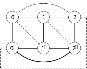
Thin solid edges have weight \(1\); the thick lower triangle has weight \(2\); dashed edges have weight \(1/2\). The outer dashed edge joins \(2\) to \(0'\), completing the shift modulo three. Crossings without a circle are not vertices.
The simultaneous rotation \(x\mapsto x+1\) generates \(C_3\). It is the entire weight-preserving vertex automorphism group. The weighted degrees \(7/2\) and \(11/2\) distinguish the two layers. The interlayer edges of weight \(1\) force the same permutation \(\pi \) on both layers, and those of weight \(1/2\) force \(\pi (x+1)=\pi (x)+1\). Thus only the three rotations remain.
The real representation is \(\mathbb R^6\cong \mathbb R^{\oplus 2}\oplus W^{\oplus 2}\), where \(W\) is the two-dimensional rotation representation and has \(D=\mathbb C\) by Proposition 13.4. The commutant is \(M_2(\mathbb R)\times M_2(\mathbb C)\), of real dimension \(4+8=12\). Its orbitals are the 4 choices of ordered layers and three differences \(y-x\). The symmetric dimension is \(3+4=7\): there are two diagonal orbits, two within-layer edge orbits and three interlayer pair orbits.
Use normalized constant vectors on the two layers for the trivial sector. For the other sector put \(\zeta =e^{2\pi i/3}\) and represent its upper values by \(f(x)=\sqrt {2/3}\operatorname {Re}(z\zeta ^{-x})\), and its lower values by the same formula with \(z'\). This is an isometry from \(\mathbb C^2\) with its real Euclidean inner product to the four-dimensional sector. Evaluating the edge energy gives \[\begin {aligned} Q_{\mathrm {triv}}&= \begin {pmatrix}5/2&-3/2\\-3/2&5/2\end {pmatrix},\\ Q_{\mathbb C}&= \begin {pmatrix} 11/2&-3/4+i\sqrt3/4\\ -3/4-i\sqrt3/4&17/2 \end {pmatrix}. \end {aligned}\] Indeed the diagonal Fourier entries are \(1+3a+u+v\) and \(1+3b+u+v\); the upper-right entry is \(-u-v\zeta ^{-1}\). The trivial eigenvalues are \(1,4\). The complex block has trace \(14\), determinant \(46\), and eigenvalues \(7-\sqrt 3,7+\sqrt 3\), each repeated twice over the reals. Hence \[\det _{\mathbb R}Q=4\cdot 46^2=8464.\] The square is required by the real determinant convention.
The imaginary entry records the shift in the declared Fourier coordinates. Rephasing one coordinate can make this single Hermitian matrix real; the intrinsic complex feature is the full commutant \(M_2(\mathbb C)\), not an obstruction to diagonalizing one positive operator. This calculation adapts the cyclic Fourier modes of Example 12.7, based on [serre1977linear, Section 5.1, p. 35].
Example 13.6. All real types in a binary tetrahedral Cayley graph [fdip-0053]AGENTDRAFTED
- November 1, 2026
Example 13.6. All real types in a binary tetrahedral Cayley graph [fdip-0053]AGENTDRAFTED
- November 1, 2026
Let \(T=2T\) be the 24 Hurwitz units, with \(\omega =(-1+i+j+k)/2\), and take the inverse-closed generating set \[S=\{i,-i,j,-j,k,-k,\omega ,\bar \omega \}.\] Give each unordered edge \(\{g,gs\}\) weight one, counting it once. There are no loops, the degree is 8, and left multiplication acts by signed graph symmetries. On \(\mathbb R^T\) the Laplacian is \[(Lf)(g)=8f(g)-\sum _{s\in S}f(gs).\] The underlying group construction is [voight2021quaternion, Section 11.2, pp. 166-168]. The following spectrum and blocks are calculations for this particular generating set.
The quotient \(T/Q_8\cong C_3\) gives the character \(\lambda (\omega )=\zeta =e^{2\pi i/3}\), \(\lambda |_{Q_8}=1\). Let \(\sigma \) be the defining two-dimensional complex quaternion representation, with \(\chi _\sigma (q)=2\operatorname {Re}q\), and let \(\tau \) act by quaternion conjugation on \(\operatorname {span}_{\mathbb R}\{i,j,k\}\). Its character is \(4(\operatorname {Re}q)^2-1\). The 7 conjugacy classes and their characters are \[\begin {array}{c|rrrrrrr} q&1&-1&i&\omega &-\omega &\omega ^2&-\omega ^2\\\hline |[q]|&1&1&6&4&4&4&4\\ \lambda ^j&1&1&1&\zeta ^j&\zeta ^j&\zeta ^{2j}&\zeta ^{2j}\\ \sigma \lambda ^j&2&-2&0&-\zeta ^j&\zeta ^j&-\zeta ^{2j}&\zeta ^{2j}\\ \tau &3&3&-1&0&0&0&0 \end {array}\] with \(j=0,1,2\). The class of \(i\) comprises \(\{\pm i,\pm j,\pm k\}\); each remaining class is determined by its \(Q_8\)-coset and real part. These descriptions follow by conjugating the explicit Hurwitz units.
Using the displayed sizes, the character inner products are \(\delta _{\alpha \beta }\) and the sum of squared degrees is \(3\cdot 1^2+3\cdot 2^2+3^2=24\). Thus the 7 characters are irreducible, inequivalent and complete. Squaring sends the first three classes to \(1,1,-1\), the two \(\pm \omega \) classes to \([\omega ^2]\), and the two \(\pm \omega ^2\) classes to \([\omega ]\). Substitution into \(|T|^{-1}\sum _g\chi (g^2)\) gives indicators \(1,0,0\) for \(1,\lambda ,\lambda ^2\), \(-1,0,0\) for \(\sigma ,\sigma \lambda ,\sigma \lambda ^2\), and \(1\) for \(\tau \). For example the numerator for \(\sigma \) is \(2+2-12-16=-24\); for \(\sigma \lambda \) it is \(4-12-8(\zeta +\zeta ^2)=0\). The real-type bridge therefore gives \[\operatorname {End}_T(\mathbb R^T) \cong \mathbb R\times \mathbb C\times M_3(\mathbb R) \times \mathbb H\times M_2(\mathbb C).\] Here the regular real multiplicity is \(m_\Xi =\dim _{D_\Xi }W_\Xi \): a real simple matrix algebra \(M_r(D)\) has \(r\) column copies of its defining module, as in Proposition [fcap-0042].
Fourier decomposition of right translation gives, up to the chosen dual-basis convention, the block \(8I-\sum _{s\in S}\pi (s)\). Its adjoint or transpose gives the same spectra and determinants, since \(S=S^{-1}\). The multiplicity matrices are as follows; in the table \(m\) is multiplicity, not the mass parameter: \[\begin {array}{c|c|c|c|c} W\text { type}&D&m&\dim _{\mathbb R}W&L_\Xi \\\hline 1&\mathbb R&1&1&0\\ \lambda ,\bar \lambda &\mathbb C&1&2&3\\ \tau &\mathbb R&3&3&11I_3-J_3\\ \sigma &\mathbb H&1&4&9\\ \sigma \lambda ,\sigma \bar \lambda &\mathbb C&2&4&\operatorname {diag}(6,9) \end {array}\] Here \(J_3\) is the all-ones matrix. For \(\tau \), the 6 \(\pm i,\pm j,\pm k\) contribute \(-2I_3\), while \(\tau (\omega )+\tau (\bar \omega )=J_3-I_3\); the block has eigenvalues \(8,11,11\). For \(\sigma \) the 6 contributions cancel and \(\sigma (\omega )+\sigma (\bar \omega )=-I_2\), giving \(9\). For \(\sigma \lambda \), diagonalize \(\sigma (\omega )\) with eigenvalues \(\zeta ,\zeta ^2\). The twisted adjacency sum has eigenvalues \(-1,2\), giving \(9,6\). The nonreal linear pair has adjacency eigenvalue \(6+\zeta +\zeta ^2=5\).
The real sector dimensions are \(1,2,9,4,8\), summing to \(24\). Consequently \[\operatorname {spec}(L)=\{0,3^{[2]},6^{[4]},8^{[3]},9^{[8]},11^{[6]}\},\] where brackets denote eigenvalue multiplicity. For a mass squared \(a>0\), set \(Q=L+aI\); every block receives the same shift and \[\begin {aligned} \det _{\mathbb R}Q={}&a(a+3)^2(a+6)^4\\ &\cdot (a+8)^3(a+9)^8(a+11)^6. \end {aligned}\] The complex and quaternionic exponents are real dimensions, not complex degrees copied without descent. The commutant dimension is \(24\); the symmetric dimension is \(13\), also the number of inversion orbits in \(T\), since only \(1,-1\) are self-inverse. These are finite graph calculations; the possible physical interpretations discussed in Remark [fgap-0018] are separate hypotheses.
14. Gaussian laws over symmetry sectors [fdip-0054]AGENTDRAFTED
- November 1, 2026
14. Gaussian laws over symmetry sectors [fdip-0054]AGENTDRAFTED
- November 1, 2026
The real isotypic projectors split a field space, and the positive multiplicity matrices describe its symmetry-preserving precisions. For a real Gaussian field this becomes a product of independent sector laws, with real dimensions and normalizers fixed by the scalar type. The result extends the two-sector product law.
If the retained vertices form a union of group orbits, elimination can be performed separately in each sector. Symmetry survives, but the retained precision can change: keeping every other vertex of a cycle produces a new cycle with different weight and mass. Its exact periodic covariance explains the change of decay scale without identifying a finite ring with an infinite lattice.
Theorem 14.1. Independent Gaussian laws on real isotypic sectors [fdip-0055]AGENTDRAFTED
- November 1, 2026
Theorem 14.1. Independent Gaussian laws on real isotypic sectors [fdip-0055]AGENTDRAFTED
- November 1, 2026
Let a finite group \(G\) act orthogonally on a finite-dimensional real inner-product space \(H\), and let \(Q>0\) be self-adjoint and \(G\)-equivariant. Write the orthogonal isotypic projectors as \(E_\Xi \), put \(H_\Xi =E_\Xi H\), and omit the zero sectors. Use induced Euclidean volumes and uncompleted Borel sigma-algebras. For the normalized Gaussian law \(\mu _Q\), the map \[\mathcal D:H\longrightarrow \prod _\Xi H_\Xi , \qquad z\longmapsto (E_\Xi z)_\Xi \] satisfies \[\mathcal D_*\mu _Q=\bigotimes _\Xi \mu _{Q|_{H_\Xi }}. \qquad Z_Q=\prod _\Xi Z_{Q|_{H_\Xi }}.\] Thus the projected fields are independent. Each has covariance \((Q|_{H_\Xi })^{-1}\) on its own real sector.
In the multiplicity coordinates, set \(D_\Xi =\operatorname {End}_G(W_\Xi )\), \(r_\Xi =\dim _{D_\Xi }W_\Xi \), and \(d_\Xi =\dim _{\mathbb R}D_\Xi \in \{1,2,4\}\). Write \(Q_\Xi \in M_{m_\Xi }(D_\Xi )\) for the multiplicity matrix; it is not the entire real-sector matrix. Then \[\begin {aligned} \det _{\mathbb R}Q &=\prod _\Xi \det _{\mathbb R} (Q_\Xi :D_\Xi ^{m_\Xi }\to D_\Xi ^{m_\Xi })^{r_\Xi },\\ Z_{Q|_{H_\Xi }} &=\frac {(2\pi )^{m_\Xi r_\Xi d_\Xi/2}} {\det _{\mathbb R}(Q_\Xi )^{r_\Xi/2}}. \end {aligned}\] The determinants in these formulas are ordinary determinants of real linear operators, including when \(D_\Xi =\mathbb H\).
Proof.
- November 1, 2026
Proof.
- November 1, 2026
The projectors are self-adjoint, mutually orthogonal and sum to \(I\). Addition from the product of their images is an isometry inverse to \(\mathcal D\). Concatenated orthonormal bases identify the orthogonal product volume with volume on \(H\); finite products of these Borel spaces have the product Borel sigma-algebra. Commutation with every projector makes \(Q\) block diagonal, so its positive quadratic form is the sum of its sector quadratic forms. The exponential weight therefore factors.
Each restricted precision is positive, and the Gaussian normalizer theorem makes every sector integral finite and positive. Nonnegative Tonelli gives the product of normalizers. Integrating the factored density on a Borel rectangle gives the product of its sector probabilities; uniqueness of finite measures on the rectangle-generated sigma-algebra gives the stated product law. This is the same measure argument as in Theorem 11.5, now for the finite family of projectors. The inverse-precision covariance theorem applies to each factor. Empty sectors have unit normalizer and their one-point law.
For the determinant, the real-sector matrix is the direct sum of \(r_\Xi \) identical real operators \(Q_\Xi \) on \(D_\Xi ^{m_\Xi }\), by the orthonormal scalar-column construction of Corollary 13.2. Determinants multiply under real direct sums. If the positive Hermitian eigenvalues of \(Q_\Xi \) are \(\lambda _1,\ldots ,\lambda _{m_\Xi }\), its real determinant is \(\prod _j\lambda _j^{d_\Xi }\). Substitution into the real Gaussian normalizer gives the displayed formula.
For the twisted prism, the trivial multiplicity matrix has determinant \(4\), while the complex matrix has complex determinant \(46\). Both have \(r_\Xi =1\), so \(\det _{\mathbb R}Q=4\cdot 46^2=8464\) and \(Z_Q=(2\pi )^3/92\). For the binary tetrahedral Cayley graph, write \(a=m^2>0\). The 5 real sectors give the following factors: \[\begin {array}{c|c|c} D_\Xi &r_\Xi &\det _{\mathbb R}(Q|_{H_\Xi })\\\hline \mathbb R&1&a\\ \mathbb C&1&(a+3)^2\\ \mathbb R&3&[(a+8)(a+11)^2]^3\\ \mathbb H&1&(a+9)^4\\ \mathbb C&2&[(a+6)(a+9)]^4 \end {array}\] Their product is \[\det _{\mathbb R}Q =a(a+3)^2(a+6)^4(a+8)^3(a+9)^8(a+11)^6.\] The exponents sum to \(24\), the real field dimension. The normalizer is \[Z_Q=\frac {(2\pi )^{12}}{\sqrt {\det _{\mathbb R}Q}}.\] These factors use the mass-shifted precision, not the singular Laplacian alone.
The density convention agrees with [friedli2017statistical, Theorem 8.4, p. 385] after setting its mean to zero and its covariance to \(\Sigma =Q^{-1}\). That theorem identifies the Gaussian density; the finite-group projectors and real determinant exponents are supplied by the proofs above and in Corollary 13.2.
Mathlib's
ProbabilityTheory.HasGaussianLaw.iIndepFun_of_covariance_inner
supports the independence step for a finite family of jointly
Gaussian real Hilbert-space variables. Here the family is
\(z\mapsto (E_\Xi z)_\Xi \), a linear image of the Gaussian field.
For distinct sectors and \(u\in H_\Xi \), \(v\in H_\Psi \), its
scalar cross covariance is \(\langle u,Q^{-1}v\rangle =0\),
because \(Q^{-1}\) preserves the orthogonal sectors. Thus the
declaration's zero-cross-covariance hypothesis matches this family.
It does not assert the representation-theoretic decomposition or the
real determinant exponents.
Theorem 14.2. Equivariant elimination within each sector [fdip-0056]AGENTDRAFTED
- November 1, 2026
Theorem 14.2. Equivariant elimination within each sector [fdip-0056]AGENTDRAFTED
- November 1, 2026
Let \(H=X\mathbin \perp Y\) be a finite-dimensional orthogonal real representation of a finite group \(G\), with both summands \(G\)-stable. Let the positive self-adjoint equivariant precision be \[Q=\begin {pmatrix}A&B\\B^*&C\end {pmatrix}, \qquad B:Y\to X.\] Then \(C>0\), and the retained precision \(S=A-BC^{-1}B^*:X\to X\) is positive, self-adjoint and \(G\)-equivariant. For every real irreducible type \(\Xi \), set \(X_\Xi =E_\Xi X\) and \(Y_\Xi =E_\Xi Y\). All block maps restrict to the indicated source and target sectors, and \[S|_{X_\Xi } =A|_{X_\Xi }-B_\Xi (C|_{Y_\Xi })^{-1}B_\Xi ^*.\] In common multiplicity coordinates, the same formula is \[S_\Xi =A_\Xi -B_\Xi C_\Xi ^{-1}B_\Xi ^*,\] where \(B_\Xi \) is an \(m_{X,\Xi }\times m_{Y,\Xi }\) matrix over \(D_\Xi \), and the products retain their displayed order.
Proof.
- November 1, 2026
Proof.
- November 1, 2026
Let \(\rho _X,\rho _Y\) denote the actions on the two summands. Equivariance of \(Q\) gives \(A\rho _X(g)=\rho _X(g)A\), \(B\rho _Y(g)=\rho _X(g)B\), and \(C\rho _Y(g)=\rho _Y(g)C\), together with the adjoint identity for \(B^*\). Positivity on \((0,y)\) makes \(C\) positive and invertible. Its inverse commutes with \(\rho _Y(g)\) by multiplying the commuting identity by \(C^{-1}\) on both sides. Hence the composite \(BC^{-1}B^*:X\to X\) and \(S\) commute with \(\rho _X(g)\). The same relations hold for the projectors, since they are real linear combinations of group actions.
Consequently \(B^*\) takes \(X_\Xi \) to \(Y_\Xi \), \(C^{-1}\) preserves \(Y_\Xi \), and \(B\) takes \(Y_\Xi \) back to \(X_\Xi \). The restriction of \(C^{-1}\) is the inverse of the restriction of \(C\), by restricting both inverse identities. This proves the typed formula, extending Proposition 11.6. Choose isometric copies of the same real irreducible in \(X_\Xi \) and \(Y_\Xi \). Intertwiners then become rectangular matrices over \(D_\Xi \) and composition becomes ordered matrix multiplication, with adjunction given by conjugate transpose. This proves the multiplicity formula also over \(\mathbb H\); no scalar factors have been commuted. An absent \(Y_\Xi \) contributes a zero composite.
Completing the real square gives \[\begin {aligned} \langle (x,y),Q(x,y)\rangle &=\langle x,Sx\rangle \\ &\quad +\langle y+C^{-1}B^*x, C(y+C^{-1}B^*x)\rangle . \end {aligned}\] Testing at \(y=-C^{-1}B^*x\) proves \(S>0\); its self-adjointness follows by adjointing the composite. This uses the real inner product, regardless of the scalar algebra of a multiplicity matrix.
Use induced Euclidean volumes and let \(\pi :H\to X\) be the orthogonal projection. For every fixed \(x\), translation in \(Y\) and the completed square give \[\int _Y e^{-\langle (x,y),Q(x,y)\rangle/2}\,d\lambda _Y(y) =Z_Ce^{-\langle x,Sx\rangle/2}.\] Nonnegative Tonelli and normalization therefore give \(Z_Q=Z_CZ_S\) and \(\pi _*\mu _Q=\mu _S\), as in positive elimination. Applying the same argument in \(X_\Xi \mathbin \perp Y_\Xi \), and then the sector product law, gives \[\begin {aligned} (\mathcal D_X)_*\pi _*\mu _Q &=\bigotimes _\Xi \mu _{S|_{X_\Xi }},\\ (\pi _\Xi )_*\mu _{Q|_{H_\Xi }} &=\mu _{S|_{X_\Xi }},\qquad Z_C=\prod _\Xi Z_{C|_{Y_\Xi }}. \end {aligned}\] Here \(\pi _\Xi :H_\Xi \to X_\Xi \); the identity \(\pi E_\Xi =E_\Xi \pi \) shows that decomposing and projecting commute as maps. Product measures then give the same commuting square as in Theorem 11.7, with all real isotypic sectors in place of the two sign sectors.
For vertex fields, the hypothesis holds when the retained set \(R\) is \(G\)-stable: take \(X=\mathbb R^R\) and \(Y=\mathbb R^{V\setminus R}\). It asserts equivariance of the induced marginal law. It does not assert that \(S=A\), the compressed precision. The cycle decimation gives a \(G\)-stable retained set with a nonzero Schur correction.
Example 14.3. Cycle decimation and periodic covariance [fdip-0057]AGENTDRAFTED
- November 1, 2026
Example 14.3. Cycle decimation and periodic covariance [fdip-0057]AGENTDRAFTED
- November 1, 2026
Take the unit-weight cycle on \(\mathbb Z/(2N)\), with \(N\ge 3\) and precision \(Q=L_{C_{2N}}+aI\), where \(a=m^2>0\). The group \(G=C_N\) acts by two-site rotations. It preserves the even retained vertices and the odd eliminated vertices. Write \(x_j=\phi _{2j}\), \(y_j=\phi _{2j+1}\) and \(q=2+a\); indices \(j\) lie in \(\mathbb Z/N\). For the shift \((Tz)_j=z_{j-1}\), the blocks are \[A=C=qI,\qquad B=-(I+T),\qquad B^*=-(I+T^{-1}).\] Thus the equivariant Schur formula gives \[\begin {aligned} S&=qI-q^{-1}(2I+T+T^{-1})\\ &=w'L_{C_N}+a'I,\\ w'&=\frac 1{2+a},\qquad a'=(2+a)-\frac 4{2+a} =\frac {a(a+4)}{a+2}>0. \end {aligned}\] Here \(L_{C_N}=2I-T-T^{-1}\). The restriction \(Q_{RR}=qI\) has no off-diagonal entries, while \(S\) has entries \(-1/q\) between adjacent retained vertices. The retained set is stable under \(G\), but the marginal precision is induced by elimination.
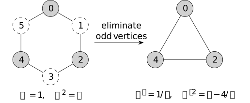
The six-cycle illustrates \(N=3\). Shaded even vertices remain; dashed odd vertices are integrated out. Each triangle edge has weight \(1/q\), and the mass squared changes from \(a\) to \(q-4/q\), with \(q=2+a\).
The finite Gaussian normalization is retained exactly: \(Z_Q=Z_CZ_S\) with \(Z_C=(2\pi/q)^{N/2}\), and the retained law is \(\mu _S\). The effective weight and mass are both part of this law. Dividing \(S\) by \(w'\) is useful for comparing its parameters, but changes the field covariance by a scalar unless the corresponding field rescaling is also made.
Put \(q=2\cosh \omega \) with \(\omega >0\). Then \[2+\frac {a'}{w'}=q^2-2=2\cosh (2\omega ).\] The doubled parameter has an exact finite-ring interpretation. For \(M\ge 3\), the covariance of precision \(w(2\cosh \eta \,I-T-T^{-1})\) on \(\mathbb Z/M\), with \(w,\eta >0\), is the periodic kernel \[\begin {aligned} K_{M,w,\eta }(r) &=\frac {e^{-\eta r}+e^{-\eta (M-r)}} {2w\sinh \eta \,(1-e^{-M\eta })},\\ &\hspace {24mm}0\le r\le M-1. \end {aligned}\] For the original and retained fields this gives \[(Q^{-1})_{0,2r} =K_{2N,1,\omega }(2r) =K_{N,w',2\omega }(r) =(S^{-1})_{0,r}.\] The equality is between covariances with their actual weights.
Proof.
- November 1, 2026
Proof.
- November 1, 2026
On the integer line, put \(h(n)=e^{-\eta |n|}/(2w\sinh \eta )\). For \(n\ne 0\), the two geometric progressions give \(w(2\cosh \eta \,h(n)-h(n-1)-h(n+1))=0\). At \(n=0\) the expression equals \((2\cosh \eta -2e^{-\eta })/(2\sinh \eta )=1\). Periodize this identity by summing \(h(r+kM)\) over \(k\in \mathbb Z\); absolute convergence permits the finite difference operation under the sum. The result is the unit point source on \(\mathbb Z/M\), so the periodized kernel is the inverse of the positive precision. Summing the geometric series gives \(K_{M,w,\eta }\).
For \(M=2N\) and even separation \(2r\), the numerator and periodic denominator equal those for \(M=N\), \(\eta =2\omega \). Their remaining constants agree because \[2w'\sinh (2\omega ) =\frac {2\sinh (2\omega )}{2\cosh \omega } =2\sinh \omega .\] This proves the covariance identity directly, in agreement with Gaussian marginalization.
In the convention that correlation length is the reciprocal decay rate of these periodized exponential images, it changes from \(\xi =1/\omega \) fine lattice units to \(\xi '=1/(2\omega )=\xi / 2\) coarse lattice units. The finite ring has two winding directions, so its covariance is not a single exponential in separation. If the old spacing is \(\ell \), the new spacing is \(2\ell \); the physical decay length \(\ell / \omega =(2\ell )/(2\omega )\) is unchanged.
The bound \(N\ge 3\) keeps the reduced graph a simple cycle. At \(N=2\), \(T=T^{-1}\) and two eliminated vertices connect the same retained pair, producing two parallel edges of weight \(1/q\), or one edge of weight \(2/q\). At \(a=0\), the algebraic formula still gives \(w'=1/2\) and \(a'=0\), the two-resistors-in-series limit. The full precision then has a constant zero mode and no normalized full-space Gaussian law. Pinning or a mean-zero constraint must be specified as in constrained massless laws; the positive-mass covariance formula is not a finite limit on the full field space.
This is a direct cycle calculation within Kron reduction, the Schur reduction of graph Laplacians with possible positive diagonal terms. Closure follows from [dorfler2011kron, Lemma 2.1, pp. 5-6]. Successive and simultaneous eliminations agree by [dorfler2011kron, Lemma 3.3, p. 14]. In that source the diagonal mass corresponds to a shunt conductance or graph self-loop. In the incidence convention used here an edge with identical endpoints has zero difference; the mass is therefore kept as the separate term \(aI\). The source supplies the general reduction context, while the periodic covariance and scale statements are proved above.
Remark 14.4. Symmetry of a marginal and restriction of a precision [fdip-0058]AGENTDRAFTED
- November 1, 2026
Remark 14.4. Symmetry of a marginal and restriction of a precision [fdip-0058]AGENTDRAFTED
- November 1, 2026
The sector laws use an ordinary orthogonal finite-group action on a real field space and a strictly positive precision. These hypotheses allow independent Gaussian factors and equivariant elimination. They do not make every stable retained subspace a reducing subspace for the precision. A stable vertex set says that its coordinate projection commutes with the group action; cycle decimation shows that it need not commute with \(Q\). The resulting Schur precision can therefore differ from the compression \(Q_{RR}\). Commuting with the group action and commuting with \(Q\) are distinct conditions.
Three other representation-theoretic questions need additional data. Projective representations and twisted group algebras record a multiplier rather than an ordinary group action; the projective obstruction explains its role. Restriction to a normal subgroup and Clifford's homogeneity theorem concern constituents under a specified subgroup inclusion; this is Clifford theory of group representations, distinct from Clifford algebras. In positive characteristic, the averaging denominator or Gaussian measure used here may be absent. None of these is supplied by real isotypic factorization alone.
15. Configuration Clifford algebras [fdip-001B]AGENTDRAFTED
- October 20, 2026
15. Configuration Clifford algebras [fdip-001B]AGENTDRAFTED
- October 20, 2026
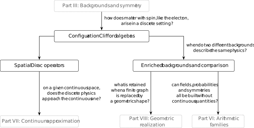
How might a discrete first-order equation acquire the internal components used to describe matter with spin? For two commuting centered differences, try \(D=a\nabla _1+b\nabla _2\). Relations \(a^2=b^2=I\) and \(ab+ba=0\) cancel the mixed term in its square. Real or complex scalars cannot satisfy them, but the two-by-two matrices \(X,Z\) do. This is an algebraic two-component example, not a derivation of electron spin. With these self-adjoint matrices and skew-adjoint centered differences, the positive square is \(-D^2\); it uses two-step shifts and differs from the nearest-neighbor Laplacian.
The common algebraic question is how a quadratic form can be encoded by products of generators. Here the configuration quadratic form determines a Clifford algebra through its square relation. Keeping the polar normalization explicit lets form-preserving maps act functorially, without identifying a quadratic map with a chosen coordinate array. This algebra encodes the supplied configuration form; it does not choose the spatial Clifford module used for Dirac operators.
Example 15.1. The configuration quadratic form and its polar forms [fdip-000O]AGENTDRAFTED
- October 17, 2026
Example 15.1. The configuration quadratic form and its polar forms [fdip-000O]AGENTDRAFTED
- October 17, 2026
For the alternating four-cycle, let \(V=\mathbb R^4\) be the space of vertex fields and let \(\delta _i(j)=\delta _{ij}\) be its coordinate vectors. These are distinct from the oriented edges \(e_i\) and the spectral vectors \(u_a\) of Example 7.19. With \(t,m>0\), put \(a=m^2\) and \(s=1+t+a\). The massive precision gives the quadratic form \[\begin {aligned} q_{t,m}(v)&=v^TQ_{t,m}v,\\ Q_{t,m}&=\begin {pmatrix} s&-1&0&-t\\-1&s&-t&0\\0&-t&s&-1\\-t&0&-1&s \end {pmatrix}. \end {aligned}\] The Euclidean action is \(\mathcal A(v)=q_{t,m}(v)/2\). The factor \(1/2\) belongs to the action; the quadratic form used below is \(q_{t,m}\) itself.
Write \(q=q_{t,m}\) and \(Q=Q_{t,m}\). The unhalved polar form and the half-polar form are respectively \[\begin {aligned} B_q(u,v)&=q(u+v)-q(u)-q(v)\\ &=2u^TQv,\\ b_q(u,v)&=\tfrac 12 B_q(u,v)=u^TQv. \end {aligned}\] Thus \(q(v)=b_q(v,v)\), while \(B_q(v,v)=2q(v)\). This is the polarization dictionary: the symmetric bilinear form called \(B\) by Meinrenken is \(b_q\), not \(B_q\). His Clifford relation uses \(2B\) [meinrenken2013clifford, Definition 2.1, p. 27].
Proof.
- October 17, 2026
Proof.
- October 17, 2026
The matrix \(Q\) is symmetric. Expanding \((u+v)^TQ(u+v)\) and canceling the two diagonal terms gives \(u^TQv+v^TQu=2u^TQv\). This is bilinear, and \(q(cv)=c^2q(v)\) for every real \(c\), so \(q\) is a quadratic form. The edge energy also gives \[\begin {aligned} q(v)={}&(v_1-v_0)^2+t(v_2-v_1)^2\\ &{}+(v_3-v_2)^2+t(v_0-v_3)^2\\ &{}+m^2\sum _{i=0}^3v_i^2. \end {aligned}\] Every term is nonnegative. If \(v\ne 0\), the last term is positive because \(m>0\); hence \(q\) is positive definite.
Mathlib's Matrix.toQuadraticForm' constructs this
matrix quadratic form. Its underlying
LinearMap.BilinMap.toQuadraticMap sends a bilinear map
\(b\) to \(v\mapsto b(v,v)\); here \(b(u,v)=u^TQv\).
The definition QuadraticMap.polar is unhalved.
These generic constructions supply the conventions; the displayed
matrix and positivity calculation specify this example.
The 4 coordinates are configuration directions, one per vertex. Positive definiteness therefore describes a form on field space. It supplies no Lorentzian spacetime metric. Changing \(t,m\) changes this form and the Gaussian state, even though the half-turn action stays fixed.
Proposition 15.2. The Clifford algebra of the configuration form [fdip-000P]AGENTDRAFTED
- October 17, 2026
Proposition 15.2. The Clifford algebra of the configuration form [fdip-000P]AGENTDRAFTED
- October 17, 2026
Let \(k\) be a commutative ring, \(M\) a \(k\)-module and \(q:M\to k\) a quadratic form. Use the tensor algebra and the square-quotient convention for the Clifford algebra: \[\operatorname {Cl}(q)=T_k(M)/I_q,\] where \(I_q\) is the two-sided ideal generated by \(v\otimes v-q(v)1\) for all \(v\in M\). The canonical linear map \(\iota _q:M\to \operatorname {Cl}(q)\) satisfies \(\iota _q(v)^2=q(v)1\). Scalars in this formula mean their images under the algebra's structure map. No invertibility of \(2\) is required for this construction.
For every unital associative \(k\)-algebra \(A\), a linear map \(f:M\to A\) extends to a unique unital \(k\)-algebra homomorphism \(\widehat f:\operatorname {Cl}(q)\to A\) if and only if \[f(v)^2=q(v)1_A\qquad (v\in M).\] This is the Clifford lift and its universal property.
Proof.
- October 17, 2026
Proof.
- October 17, 2026
Necessity follows by applying an algebra homomorphism to the square relation. For sufficiency, send a pure tensor to its ordered product, \[v_1\otimes \cdots \otimes v_r\longmapsto f(v_1)\cdots f(v_r),\] and send \(c\in k=T_k^0(M)\) to \(c1_A\). The product is multilinear because \(f\) is linear, multiplication in \(A\) is distributive, and the scalar images are central. The tensor-product universal property therefore gives a linear map on each tensor power. Their direct sum defines a linear map \(F:T_k(M)\to A\). Concatenation of pure tensors becomes multiplication of their ordered products. Distributivity then proves multiplicativity on all finite sums, and the degree-zero formula preserves the unit and scalars. Every generator of \(I_q\) maps to \(f(v)^2-q(v)1_A=0\); multiplicativity makes every element of the two-sided ideal map to zero. Thus \(F\) descends to \(\widehat f\). Every tensor is a finite linear combination of pure tensors, whose images in the quotient are products of the \(\iota _q(v)\). An algebra map with the prescribed generator values must have the displayed value on each such product and on every scalar. This proves uniqueness.
Linearity and the square relation give the anticommutator: \[\begin {gathered} \iota _q(u)\iota _q(v)+\iota _q(v)\iota _q(u)\\ =\bigl (q(u+v)-q(u)-q(v)\bigr )1\\ =B_q(u,v)1. \end {gathered}\] Indeed, expand \((\iota _q(u)+\iota _q(v))^2\) and subtract the two squares. This uses no division by \(2\). When \(2\) is invertible, \(b_q=B_q/2\) exists and the relation becomes \(\iota _q(u)\iota _q(v)+\iota _q(v)\iota _q(u)=2b_q(u,v)1\). Conversely that relation with \(u=v\) recovers the square relation by cancellation of \(2\). Thus the two presentations agree in this case. Without that hypothesis, the anticommutator alone need not recover the squares.
Meinrenken gives the bilinear presentation in
[meinrenken2013clifford, Definition 2.1, p. 27]
and the universal property in
[meinrenken2013clifford, Proposition 2.2 and Remark 2.2, p. 29].
His chapter assumes a finite-dimensional vector space over a
characteristic-zero field (p. 23); Remark 2.2 includes the ordinary
algebra formulation. The direct argument above supplies the stated
commutative-ring generality. Mathlib's
CliffordAlgebra.ι_sq_scalar,
CliffordAlgebra.lift,
CliffordAlgebra.lift_unique and
CliffordAlgebra.ι_mul_ι_add_swap
provide these respective generic square, extension, uniqueness and
unhalved-polar statements.
Now take the real configuration form and put \(c_i=\iota _q(\delta _i)\). Write \(\{x,y\}=xy+yx\) for the anticommutator. The matrix entries give \[\begin {aligned} c_i^2&=s1\quad (i=0,1,2,3),\\ \{c_0,c_1\}&=\{c_2,c_3\}=-2\,1,\\ \{c_1,c_2\}&=\{c_3,c_0\}=-2t\,1,\\ \{c_0,c_2\}&=\{c_1,c_3\}=0. \end {aligned}\] These follow from \(q(\delta _i)=Q_{ii}=s\) and \(b_q(\delta _i,\delta _j)=Q_{ij}\). In particular the squares are positive in this convention. The opposite-sign convention would use \(-q\).
For this real form, both the scalar map and \(\iota _q\) are
injective. Here is the exterior algebra argument of
[meinrenken2013clifford, Proposition 2.1, p. 28], with its
operator identities made explicit. On \(\bigwedge V\), let
\(\epsilon (v)\omega =v\wedge \omega \), and define contraction by
\[d_v(1)=0,\]
\[\begin {gathered}
d_v(w_1\wedge \cdots \wedge w_r)\\
=\sum _{j=1}^r(-1)^{j-1}b_q(v,w_j)\\
\quad \cdot w_1\wedge \cdots \widehat {w_j}\cdots \wedge w_r.
\end {gathered}\]
The alternating multilinear expression defines a linear operator
on the exterior algebra. Exterior alternation gives
\(\epsilon (v)^2=0\). In \(d_v^2\), each pair of removed positions
occurs twice with opposite signs and the same scalar coefficient,
so \(d_v^2=0\). Separating the first term of \(d_v(v\wedge \omega )\)
gives
\[d_v\epsilon (v)+\epsilon (v)d_v=b_q(v,v)I.\]
Consequently \(C(v)=\epsilon (v)+d_v\) is linear in \(v\) and
\(C(v)^2=q(v)I\). The universal property gives a unital algebra
map \(\rho :\operatorname {Cl}(q)\to \operatorname {End}_{\mathbb R}(\bigwedge V)\).
It satisfies \(\rho (\iota _q(v))1=v\) and \(\rho (r1)1=r1\).
Since \(\bigwedge ^1 V=V\) and \(\bigwedge ^0V=\mathbb R\),
these equations prove both injections. The contraction identities
are also recorded in [meinrenken2013clifford, Section 2.1.3, pp. 25-26].
TauCeti's CliffordAlgebra.ι_injective and
CliffordAlgebra.algebraMap_injective
give the corresponding injections for an arbitrary quadratic form
over a commutative ring with invertible \(2\).
The exterior action just used proves faithfulness on vectors and scalars; it does not assert that \(\rho \) is a faithful algebra representation. Nor does this construction select a physical spinor module, a positive expectation on the Clifford algebra, or a differential operator. The earlier Gaussian expectation acts on polynomial observables of vertex fields; an expectation on this new algebra would require a specified construction.
Theorem 15.3. Form-preserving maps and the half-turn Clifford automorphism [fdip-000Q]AGENTDRAFTED
- October 17, 2026
Theorem 15.3. Form-preserving maps and the half-turn Clifford automorphism [fdip-000Q]AGENTDRAFTED
- October 17, 2026
Let \(k\) be a commutative ring, \(M_1,M_2\) be \(k\)-modules with quadratic forms \(q_1,q_2\), and let \(f:M_1\to M_2\) be linear with \[q_2(f(v))=q_1(v)\qquad (v\in M_1).\] This form-preserving map induces a unique unital \(k\)-algebra map \[\operatorname {Cl}(f):\operatorname {Cl}(q_1)\longrightarrow \operatorname {Cl}(q_2)\] satisfying \(\operatorname {Cl}(f)(\iota _1(v))=\iota _2(f(v))\). This is the underlying Clifford map in isometry transport. It requires no inverse for \(f\). The defining square is:
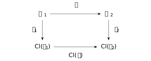
The top and vertical arrows are linear maps; the bottom arrow is a unital algebra map. The square commutes as a square of linear maps. For composable form-preserving maps \(f,g\), \[\begin {aligned} \operatorname {Cl}(\operatorname {id})&=\operatorname {id},\\ \operatorname {Cl}(g\circ f)&=\operatorname {Cl}(g)\circ \operatorname {Cl}(f). \end {aligned}\] If \(f\) is a linear isomorphism, \(\operatorname {Cl}(f)\) is an algebra isomorphism with inverse \(\operatorname {Cl}(f^{-1})\).
Proof.
- October 17, 2026
Proof.
- October 17, 2026
The linear map \(v\mapsto \iota _2(f(v))\) has square \(q_2(f(v))1=q_1(v)1\). Apply the universal property to obtain the unique extension. For the identity, the induced map and the identity algebra map agree on every generator, hence are equal by uniqueness. For composition, both proposed maps send \(\iota _1(v)\) to \(\iota _3(g(f(v)))\); uniqueness again proves equality. If \(f\) is invertible, set \(v=f^{-1}(w)\) in form preservation to get \(q_1(f^{-1}(w))=q_2(w)\). Thus the inverse is also form-preserving. The two composition identities give mutually inverse algebra maps.
Meinrenken derives this functoriality for bilinear-form-preserving
maps in [meinrenken2013clifford, Section 2.2.2, p. 29].
Over his characteristic-zero field, polarization equates that
condition with preservation of \(q\). The proof here applies
directly to quadratic forms over commutative rings. Mathlib's
CliffordAlgebra.map,
CliffordAlgebra.map_apply_ι,
CliffordAlgebra.map_id,
CliffordAlgebra.map_comp_map and
CliffordAlgebra.equivOfIsometry
provide the extension, generator equation, identity, composition
and inverse construction. Their input is a linear map preserving
the quadratic form, or a linear equivalence for the last result.
Return to \(q=q_{t,m}\) on \(V=\mathbb R^4\). The same half-turn sends \(\delta _i\) to \(\delta _{i+2}\), with indices modulo \(4\). It satisfies \(P^2=I\) and \(P^TQP=Q\), so \(q(Pv)=q(v)\). Therefore \[\begin {aligned} \Theta &=\operatorname {Cl}(P),\\ \Theta (c_i)&=c_{i+2},\qquad \Theta ^2=\operatorname {id}. \end {aligned}\] The matrix equation follows by shifting both indices of \(Q\) by two: its diagonal, its paired off-diagonal entries \(-1\) and \(-t\), and its zeros are preserved. Composition gives \(\Theta ^2=\operatorname {Cl}(P^2)=\operatorname {id}\). Moreover \(\delta _0\ne \delta _2\), so injectivity of \(\iota _q\) gives \(c_0\ne c_2\). Thus \(\Theta \) is nontrivial and has order exactly two.
The real half-turn sectors
\(V_\pm =\ker (P\mp I)\) are orthogonal for \(b_q\). Indeed,
\(P^TQP=Q\) gives \(b_q(Pu,Pv)=b_q(u,v)\). For
\(u\in V_+\) and \(v\in V_-\), the left side is
\(b_q(u,-v)=-b_q(u,v)\). Over \(\mathbb R\) this forces
\(b_q(u,v)=0\), and hence
\[\iota _q(u)\iota _q(v)=-\iota _q(v)\iota _q(u).\]
This is the generic orthogonality consequence
CliffordAlgebra.ι_mul_ι_comm_of_isOrtho.
The cross-sector vector generators anticommute; the direct sum
of sectors does not make them commuting factors of an ordinary
tensor-product algebra.
Preservation of the form is essential. Compare \(q_{1,1}\) and \(q_{2,1}\) while keeping the coordinate labels unchanged. At \(\delta _0\), \[q_{1,1}(\delta _0)=3,\qquad q_{2,1}(\delta _0)=4.\] Thus the identity linear map is not form-preserving. Write \(c_i^{(1)},c_i^{(2)}\) for the two sets of generators. A unital real algebra map with \(c_i^{(1)}\mapsto c_i^{(2)}\) would send \((c_0^{(1)})^2=3\,1\) to \((c_0^{(2)})^2=3\,1\), but the target square is \(4\,1\). Its injective scalar map rules this out. This excludes precisely the unchanged-label assignment. It does not exclude other isometries between the positive forms or an abstract isomorphism of their Clifford algebras.
The construction transports a supplied configuration form and its discrete symmetry. It supplies no spacetime derivative, Dirac operator or Lorentzian interpretation. Those structures need additional data and compatibility conditions.
16. Spatial Dirac operators [fdip-001C]AGENTDRAFTED
- October 20, 2026
16. Spatial Dirac operators [fdip-001C]AGENTDRAFTED
- October 20, 2026
A periodic spatial grid carries a different Clifford-module problem from the configuration space. A separately chosen complex Clifford module couples to centered differences. The square and Fourier blocks of the resulting Dirac operator can be calculated exactly. Its zero modes and comparison with nearest-neighbor differences show why a Clifford construction alone does not determine the desired kinetic operator or a continuum limit.
Definition 16.1. A centered Dirac operator on a finite periodic grid [fdip-000R]AGENTDRAFTED
- October 17, 2026
Definition 16.1. A centered Dirac operator on a finite periodic grid [fdip-000R]AGENTDRAFTED
- October 17, 2026
To couple Clifford multiplication to spatial differences, fix an integer \(d\ge 1\) and periods \(N_j\ge 3\) for \(1\le j\le d\). The periodic grid and its scalar fields are \[\begin {aligned} \Lambda &=\prod _{j=1}^d\mathbb Z/N_j\mathbb Z,\\ M&=\prod _{j=1}^d N_j,\qquad H=\mathbb C^\Lambda . \end {aligned}\] Write \(e_j\in \Lambda \) for the unit step in coordinate \(j\). Addition is periodic and the lattice spacing is one. Extend the counting pairing to the Hermitian inner product \[\langle f,g\rangle _H =\sum _{x\in \Lambda }\overline {f(x)}g(x),\] conjugate-linear in the first slot.
The spatial quadratic form is \[q_{\mathrm {sp}}(z)=\sum _{j=1}^d z_j^2 \qquad (z\in \mathbb C^d).\] It is distinct from the Hermitian norm squared \(\sum _j|z_j|^2\) and from the real four-field configuration form. For example, at \(i\varepsilon _1\), where \(\varepsilon _j\) is the standard basis of \(\mathbb C^d\), the quadratic value is \(-1\) and the Hermitian norm squared is \(1\). The grid steps \(e_j\), these complex coordinate vectors, and the 4 configuration coordinates have different carriers.
Choose \(S=(\mathbb C^2)^{\otimes d}\) with its standard tensor
basis and product Hermitian inner product. In the
Pauli convention, take
\[X=\begin {pmatrix}0&1\\1&0\end {pmatrix},\qquad
Z=\begin {pmatrix}1&0\\0&-1\end {pmatrix},\]
and put \(I=I_2\) and
\[\gamma _j=Z^{\otimes (j-1)}\otimes X
\otimes I^{\otimes (d-j)}.\]
An empty tensor product contributes the scalar identity.
Direct multiplication gives \(X^*=X\), \(Z^*=Z\),
\(X^2=Z^2=I\) and \(XZ=-ZX\). Ordinary tensor products obey
\[\begin {aligned}
(A\otimes B)^*&=A^*\otimes B^*,\\
(A\otimes B)(C\otimes E)&=AC\otimes BE.
\end {aligned}\]
The product formula follows on pure tensors, which span; the
adjoint formula follows from the product inner product on such
tensors. Thus \(\gamma _j^*=\gamma _j\) and
\(\gamma _j^2=I_S\). For \(i<j\), the only anticommuting slot is
\(i\), where \(X\) meets \(Z\). Before it both factors are \(Z\);
after it at least one factor is \(I\). Hence
\[\gamma _i\gamma _j+\gamma _j\gamma _i
=2\delta _{ij}I_S.\]
Mathlib's Matrix.kronecker,
Matrix.mul_kronecker_mul,
Matrix.conjTranspose_kronecker and
Matrix.one_kronecker_one give the corresponding
matrix construction and identities. Iterating them requires
identifying the product-index bases.
The complex-linear map \(c:\mathbb C^d\to \operatorname {End}_{\mathbb C}(S)\)
defined by \(c(z)=\sum _j z_j\gamma _j\) satisfies
\[\begin {aligned}
c(z)^2&=\sum _j z_j^2 I_S\\
&\quad +\sum _{i<j}z_i z_j
(\gamma _i\gamma _j+\gamma _j\gamma _i)\\
&=q_{\mathrm {sp}}(z)I_S.
\end {aligned}\]
The Clifford universal property therefore gives a
unique unital complex-algebra map
\[\begin {aligned}
\rho :\operatorname {Cl}(q_{\mathrm {sp}})&\longrightarrow
\operatorname {End}_{\mathbb C}(S),\\
\rho (\iota (\varepsilon _j))&=\gamma _j.
\end {aligned}\]
This makes \(S\) a Clifford module, in the
module-map convention.
The ordinary-algebra universal property is stated in
[meinrenken2013clifford, Proposition 2.2 and Remark 2.2, p. 29].
Its bilinear form is \(b(z,w)=\sum _j z_jw_j\), with relation
\(uv+vu=2b(u,v)1\); see
[meinrenken2013clifford, Definition 2.1, p. 27].
The displayed square identity is precisely the input required
by CliffordAlgebra.lift over \(\mathbb C\).
This chosen module is reducible. The involution \[J=I^{\otimes (d-1)}\otimes X\] commutes with every \(\gamma _j\): its last factor meets either \(I\) or \(X\), and its other factors are identities. Its two eigenspaces are \[S_\pm =(\mathbb C^2)^{\otimes (d-1)} \otimes \mathbb C(1,\pm 1).\] Both are nonzero and have dimension \(2^{d-1}\). Commutation with \(J\) makes them invariant under every generator and hence under the generated Clifford action. We use \(\dim S=2^d\); no minimality or faithfulness of this representation is needed.
Extend the cyclic shift coordinatewise: \[(T_j f)(x)=f(x+e_j).\] Its inverse shifts by \(-e_j\). Reindexing \(y=x+e_j\) gives \[\begin {aligned} \langle T_jf,g\rangle _H &=\sum _y\overline {f(y)}g(y-e_j)\\ &=\langle f,T_j^{-1}g\rangle _H. \end {aligned}\] Thus \(T_j^*=T_j^{-1}\), so \(T_j\) is unitary. The shifts and their inverses commute, since addition in \(\Lambda \) commutes. The centered differences are the endomorphisms \[\nabla _j=(T_j-T_j^{-1})/2.\] They commute and satisfy \(\nabla _j^*=-\nabla _j\). Their source and target are both \(H\), unlike a general vertex-to-edge incidence map.
Set \(K=S\otimes _{\mathbb C}H\), with \(\langle s\otimes f,t\otimes g\rangle _K =\langle s,t\rangle _S\langle f,g\rangle _H\). Identify \(s\otimes f\) with the field \(x\mapsto f(x)s\). The centered Dirac operator is \[D=\sum _{j=1}^d\gamma _j\otimes \nabla _j.\] Equivalently, \[\begin {aligned} (D\psi )(x) &=\frac 12\sum _{j=1}^d\gamma _j\psi (x+e_j)\\ &\quad -\frac 12\sum _{j=1}^d\gamma _j\psi (x-e_j). \end {aligned}\] For \(d=1\), this is \(X\) applied to the ordinary centered difference of a two-component field. Wingate's gauge-covariant centered difference reduces to this difference when all links are one and the spacing is one [wingate2025lattice, Section 9.1, Equation (9.2), p. 19]. The finite grid and tensor module here are specified directly; this construction introduces no Grassmann integration or gauge field. The Lorentz-sign gamma algebra is a different choice of form, scalar field and representation.
Theorem 16.2. The Dirac square and its finite Fourier blocks [fdip-000S]AGENTDRAFTED
- October 17, 2026
Theorem 16.2. The Dirac square and its finite Fourier blocks [fdip-000S]AGENTDRAFTED
- October 17, 2026
For the periodic grid and Clifford module, the centered Dirac operator is skew-adjoint and has square \[\begin {aligned} D^*&=-D,\\ D^2&=I_S\otimes \sum _{j=1}^d\nabla _j^2,\\ -D^2&=\frac 14 I_S\otimes \sum _{j=1}^d(2I_H-T_j^2-T_j^{-2}). \end {aligned}\] In particular \(-D^2=D^*D\) is positive semidefinite. Its complete finite Fourier decomposition has blocks \[\begin {aligned} D(p)&=i\sum _{j=1}^d\gamma _j\sin p_j,\\ -D(p)^2&=s(p)I_S,\\ s(p)&=\sum _{j=1}^d\sin ^2p_j, \end {aligned}\] where \(p_j=2\pi r_j/N_j\) and \(0\le r_j<N_j\). The sine convention agrees with the free propagator in [wingate2025lattice, Section 9.1, Equations (9.6)-(9.7), p. 20] after setting the spacing to one. The finite decomposition and square are proved below.
Proof.
- October 17, 2026
Proof.
- October 17, 2026
The tensor adjoint formula and \(\gamma _j^*=\gamma _j\), \(\nabla _j^*=-\nabla _j\) give \((\gamma _j\otimes \nabla _j)^* =-\gamma _j\otimes \nabla _j\); adding proves \(D^*=-D\). In the square, every diagonal term is \(\gamma _j^2\otimes \nabla _j^2=I_S\otimes \nabla _j^2\). For \(i<j\), the paired off-diagonal terms are \[\begin {gathered} \gamma _i\gamma _j\otimes \nabla _i\nabla _j +\gamma _j\gamma _i\otimes \nabla _j\nabla _i\\ =(\gamma _i\gamma _j+\gamma _j\gamma _i) \otimes \nabla _i\nabla _j=0, \end {gathered}\] using commutation of the differences and anticommutation of the distinct gamma matrices. This proves the square formula. Expanding \(\nabla _j^2\) gives \((T_j^2-2I_H+T_j^{-2})/4\). Finally \(\langle \psi ,-D^2\psi \rangle _K =\langle D\psi ,D\psi \rangle _K\ge 0\).
Let \(\mathcal R=\prod _j\{0,\ldots ,N_j-1\}\) and, for \(r\in \mathcal R\), define the normalized character function \[\chi _r(x)=M^{-1/2} \exp \left (i\sum _{j=1}^d p_jx_j\right ).\] Choose integer representatives for \(x_j\). Changing one by \(N_j\) multiplies the exponential by \(\exp (2\pi i r_j)=1\); changing \(r_j\) by \(N_j\) likewise multiplies it by \(\exp (2\pi i x_j)=1\). Thus the function depends only on the residue classes.
For \(r,t\in \mathcal R\), put \[\zeta _j=\exp \left (\frac {2\pi i(t_j-r_j)}{N_j}\right ).\] The counting inner product factors: \[\langle \chi _r,\chi _t\rangle _H =M^{-1}\prod _{j=1}^d\sum _{k=0}^{N_j-1}\zeta _j^k.\] If \(t_j=r_j\), then \(\zeta _j=1\) and the inner sum is \(N_j\). Otherwise the chosen range of labels gives \(\zeta _j\ne 1\) and \(\zeta _j^{N_j}=1\), so \[(1-\zeta _j)\sum _{k=0}^{N_j-1}\zeta _j^k =1-\zeta _j^{N_j}=0.\] Division by \(1-\zeta _j\) makes that sum zero. Consequently \(\langle \chi _r,\chi _t\rangle _H=\delta _{rt}\). There are \(M\) such functions, and \(\dim _{\mathbb C}H=M\), as witnessed by the vertex indicators. Orthonormality gives linear independence, so these functions form a complete basis.
For a spinor-valued field, the Fourier transform and inverse therefore are \[\begin {aligned} \widehat \psi (r) &=M^{-1/2}\sum _{x\in \Lambda } e^{-i\sum _jp_jx_j}\psi (x),\\ \psi (x) &=M^{-1/2}\sum _{r\in \mathcal R} e^{i\sum _jp_jx_j}\widehat \psi (r). \end {aligned}\] For scalar fields the coefficient is \(\widehat f(r)=\langle \chi _r,f\rangle _H\); applying that basis expansion in each standard coordinate of \(S\) proves the two vector-valued formulas. Thus \[K=\bigoplus _{r\in \mathcal R} S\otimes \mathbb C\chi _r.\] The forward shift has \(T_j\chi _r=e^{ip_j}\chi _r\), hence \(\nabla _j\chi _r=i\sin p_j\,\chi _r\). Each displayed summand is invariant under \(D\), with block \(D(p)=i\sum _j\gamma _j\sin p_j\). Expanding its square using the same anticommutators gives \(D(p)^2=-s(p)I_S\).
Mathlib's LinearMap.adjoint and
LinearMap.adjoint_inner_right give the finite-dimensional
adjoint and its characterizing identity;
LinearMap.adjoint_comp reverses composition.
The relevant formal inner-product structure is the counting
Euclidean space, for example a \(\operatorname {PiLp}(2)\)
model. The raw function type's default supremum norm cannot
silently replace that structure. The translation and tensor
identifications are the direct calculations above.
Mathlib's ZMod.dft,
ZMod.dft_apply and ZMod.invDFT_apply
provide the one-coordinate Fourier equivalence: its forward
sum has a negative exponent and no normalizing factor, while
its inverse has a positive exponent and factor \(N^{-1}\).
Iterating over coordinates and scaling the forward transform
by \(M^{-1/2}\) gives the conventions above.
AddChar.wInner_cWeight_eq_boole gives generic
character orthogonality for the normalized average inner
product. Here the unscaled characters have counting norm
\(\sqrt M\); the factor \(M^{-1/2}\) makes them orthonormal.
Their explicit enumeration, the shift eigenvalues and the
spinor blocks are supplied by this finite proof.
Proposition 16.3. Zero modes and the nearest-neighbor mismatch [fdip-000T]AGENTDRAFTED
- October 17, 2026
Proposition 16.3. Zero modes and the nearest-neighbor mismatch [fdip-000T]AGENTDRAFTED
- October 17, 2026
On the periodic grid, let \(e\) be the number of even periods among \(N_1,\ldots ,N_d\). The centered Dirac operator has exactly \(2^e\) zero momentum blocks and \[\dim _{\mathbb C}\ker D=2^{d+e}.\] This is the kernel dimension for the explicitly chosen reducible module \(S\), whose dimension is \(2^d\). The unit-weight graph Laplacian \[L_{\mathrm {nn}}=\sum _{j=1}^d (2I_H-T_j-T_j^{-1})\] has only the zero momentum in its scalar kernel. Moreover \(-D^2\ne I_S\otimes L_{\mathrm {nn}}\) on every permitted grid, including grids with all periods odd. These are finite consequences of the Fourier blocks; the centered-difference convention comes from [wingate2025lattice, Section 9.1, Equations (9.2), (9.6)-(9.7), pp. 19-20].
Proof.
- October 17, 2026
Proof.
- October 17, 2026
The forward-difference factorization from Lemma 3.6, applied in each coordinate, gives \[L_{\mathrm {nn}}=\sum _j(T_j-I_H)^*(T_j-I_H).\] For \(N_j\ge 3\), each undirected nearest-neighbor edge occurs once in the corresponding squared-difference energy. On the character with momentum \(p\), the eigenvalue is \[\begin {aligned} \ell (p)&=\sum _j(2-2\cos p_j)\\ &=4\sum _j\sin ^2(p_j/2). \end {aligned}\] The positive Dirac square has scalar block \(s(p)=\sum _j\sin ^2p_j\). The double-angle identity gives \[\ell (p)-s(p)=4\sum _j\sin ^4(p_j/2).\] Choose \(r_1=1\) and the other labels zero. Since \(N_1\ge 3\), \(\sin (\pi/N_1)>0\), so the difference is strictly positive on that block. This proves the operator mismatch.
Every summand of \(s(p)\) is nonnegative. Hence \(s(p)=0\) exactly when each \(\sin p_j=0\). In the range \(0\le r_j<N_j\), this means \(r_j=0\), or \(r_j=N_j/2\) when \(N_j\) is even. There are exactly \(2^e\) choices. On each such block \(D(p)=0\) on all of \(S\). Every other block is invertible, with two-sided inverse \[D(p)^{-1}=-D(p)/s(p),\] because \(D(p)^2=-s(p)I_S\). Completeness of the Fourier basis therefore gives \(\dim \ker D=2^e\dim S=2^{d+e}\). In contrast, \(\ell (p)=0\) forces \(r_j=0\) for every \(j\); thus \(\dim \ker (I_S\otimes L_{\mathrm {nn}})=2^d\).
For \(d=1,N=4\), the alternating scalar field \(a(x)=(-1)^x\) has momentum \(p=\pi \). Its centered difference is zero, whereas \(L_{\mathrm {nn}}a=4a\). Consequently every field \(x\mapsto a(x)v\), \(v\in S\), is killed by \(D\). Together with the constant fields these give the four-dimensional kernel. Write \(K_2=(2I_H-T^2-T^{-2})/4\), so \(-D^2=I_S\otimes K_2\). The two scalar Laplacians have the following weighted graphs:
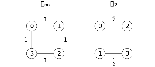
Left: the 4 unit-weight nearest-neighbor edges. Right: the two-step edges, with vertices rearranged to display the parity classes \(\{0,2\}\) and \(\{1,3\}\). At period \(4\), \(T^2=T^{-2}\), so \(K_2=(I_H-T^2)/2\): the two shift contributions of weight \(1/4\) combine into one undirected edge of weight \(1/2\) for each opposite pair. The alternating field is constant on each right-hand component, explaining its zero energy there.
For \(d=1,N=3\), momentum \(p=2\pi/3\) instead gives \[s(p)=\tfrac 34,\qquad \ell (p)=3.\] Only \(r=0\) is a zero momentum, yet the operators still differ. Thus extra exact zero momenta occur precisely when at least one period is even, whereas the square mismatch always occurs. The excluded case \(N=2\) has \(T=T^{-1}\), making its centered difference identically zero.
The finite kernel dimension above is not a physical species or chirality count. Friedan's Nielsen-Ninomiya theorem concerns free fermions on the infinite lattice \(\mathbb Z^d\) for odd \(d\), with continuous torus momenta. Its Hamiltonian is quadratic, phase invariant, translation invariant and local, with a Hermitian momentum symbol. The locality discussion reduces the Hamiltonian requirement to continuity; the internal-charge projections must be smooth. The zero set is finite and isolated, with specified relativistic Clifford-linear behavior near each zero. Under these hypotheses the total chiral index vanishes separately for each charge [friedan1982nielsen, Sections 1-2, pp. 481-484; Equations (6), (10)-(11)]. A finite sampled grid in arbitrary dimension with the chosen reducible module computes a different quantity. The odd-period example neither contradicts that theorem nor establishes a continuum limit. No Lorentzian model or factorization of the earlier weighted precision is supplied by this centered operator.
17. Enriched backgrounds and comparison [fdip-001E]AGENTDRAFTED
- October 20, 2026
17. Enriched backgrounds and comparison [fdip-001E]AGENTDRAFTED
- October 20, 2026
Which data must a comparison preserve for observables to survive? The finite background, its reference pairing and retained split already distinguish a relabeling from an arbitrary field map. The cycle trace ratio gives an observable with which to test a proposed comparison.
The enriched groupoid records allowed arrows and the data they preserve. Scalar invariants descend along those arrows without classifying all backgrounds. Quadratic isometry can forget the reference pairing or retained projection even while transporting a positive Gaussian law. Its Clifford functoriality therefore need not retain all the information required for these observables.
Example 17.1. The groupoid of enriched four-cycle backgrounds [fdip-000X]AGENTDRAFTED
- October 18, 2026
Example 17.1. The groupoid of enriched four-cycle backgrounds [fdip-000X]AGENTDRAFTED
- October 18, 2026
A classification of Gaussian backgrounds must retain the maps that transport their observables. Consider the alternating four-cycle with vertices \(V=\mathbb Z/4\mathbb Z\), forward edges \(e_i:i\to i+1\), and weights \((a,b,a,b)\), where \(a,b>0\). Choose \(m>0\) and one of \(R_0=\{0,2\}\), \(R_1=\{1,3\}\) as retained vertices. Write \(x=(a,b,m,R_j)\) and let \(X\) be the set of all these tuples. The tuple specifies a finite Gaussian background, together with its named half-turn.
More explicitly, retain the carrier, counting reference pairing, weight matrix \(W_x=\operatorname {diag}(a,b,a,b)\), and \[L_x=B^TW_xB,\qquad Q_x=L_x+m^2I.\] Here \((B\phi )_i=\phi _{i+1}-\phi _i\). For \(\phi \ne 0\), \[\begin {aligned} \phi ^TQ_x\phi &=\sum _iw_i(\phi _{i+1}-\phi _i)^2\\ &\quad +m^2\|\phi \|^2>0. \end {aligned}\] The normalized Gaussian \(\mu _{Q_x}\) is determined by this precision and coordinate Lebesgue measure. Also retain the measurable coordinate projection \(\pi _{R_j}:\mathbb R^V\to \mathbb R^{R_j}\) and the named action \(\rho (h)\delta _i=\delta _{i+2}\) of \(C_2=\{1,h\}\). The vertex basis \(\delta _i(v)=\mathbf 1_{v=i}\) is distinct from the edges \(e_i\) and the spectral vectors \(u_a\). These structures are specified or determined, rather than additional freely variable coordinates of \(X\).
Allow rotations and reflections of the underlying cycle. Put \[D_4=\langle r,s\mid r^4=s^2=1,\ srs=r^{-1}\rangle ,\] where \(r(i)=i+1\) and \(s(i)=-i\). A reflection reverses the forward orientation. Thus these arrows use the signed endpoint convention and extend the earlier strictly directed exact relabelings. For \(g=r^ks^\varepsilon \), with \(k\in \mathbb Z/4\) and \(\varepsilon \in \{0,1\}\), set \[\begin {aligned} g(i)&=k+(-1)^\varepsilon i,\\ P_g\delta _i&=\delta _{g(i)},\\ \tau _g(i)&=\begin {cases}k+i&\varepsilon =0,\\k-i-1&\varepsilon =1,\end {cases}\\ U_g\eta _i&=(-1)^\varepsilon \eta _{\tau _g(i)}. \end {aligned}\] Here \(\eta _i\) is the edge-field coordinate basis. All indices are modulo \(4\). The 8 vertex maps are distinct because their values at \(0,1\) determine \(k,\varepsilon \).
The edge indexed by \(\tau _g(i)\) has endpoints \(g(i),g(i+1)\), in forward order for a rotation and reverse order for a reflection. Consequently, for every field \(\phi \), \[\begin {aligned} (BP_g\phi )_{\tau _g(i)}&=(-1)^\varepsilon (B\phi )_i,\\ BP_g&=U_gB. \end {aligned}\] If \(k'\) denotes a second group element, endpoint transport and multiplication of the orientation signs give \[P_{k'g}=P_{k'}P_g,\qquad U_{k'g}=U_{k'}U_g.\] For an explicit group-law check, composition of \((k,\varepsilon )\) followed by \((\ell ,\eta )\) gives \[\begin {aligned} (\ell ,\eta )(k,\varepsilon ) &=(\ell +(-1)^\eta k,\eta +\varepsilon ). \end {aligned}\] The second coordinate is taken modulo two. Both coordinate maps are orthogonal, and their inverses are indexed by \(g^{-1}\).
Transport weights by \(W_{gx}=U_gW_xU_g^T\) and the retained set by \(R\mapsto gR\). The signs cancel in the diagonal weight matrix. The weights swap exactly when \(k+\varepsilon \) is odd, while \(R_j\mapsto R_{j+k\bmod 2}\). In particular, \[\begin {aligned} r(a,b,m,R_j)&=(b,a,m,R_{j+1}),\\ s(a,b,m,R_j)&=(b,a,m,R_j). \end {aligned}\] The family is closed under these maps, with mass unchanged. Using \(BP_g^T=U_g^TB\) gives \[\begin {aligned} L_{gx}&=B^TU_gW_xU_g^TB=P_gL_xP_g^T,\\ Q_{gx}&=P_gQ_xP_g^T. \end {aligned}\] Moreover \(g(i+2)=g(i)+2\), so every arrow commutes with the same named half-turn: \(P_g\rho (h)=\rho (h)P_g\).
Form the action groupoid \(D_4\ltimes X\) by setting \[\operatorname {Hom}(x,y)=\{g\in D_4:g x=y\}.\] The group element remains part of an arrow. Compose \(g:x\to y\) and \(k:y\to z\) as \(kg:x\to z\); the action law gives its target. The identity is \(1:x\to x\), the inverse is \(g^{-1}:gx\to x\), and the two inverse identities and associativity follow from the group laws. Thus every arrow is invertible, as in [stacks2017stacks, Definition 4.2.5], Tag 0018. The source, target and composition follow the set-level pattern in [stacks2017stacks, Lemma 78.15.1], Tag 0444; that lemma is stated for algebraic spaces, whereas the axioms here were checked directly for sets. \(X\) is infinite, but each orbit and its restricted groupoid is finite.
The stabilizer of the weights at \(a\ne b\) is \(\{1,r^2,rs,r^3s\}\cong C_2\times C_2\); preserving weights requires \(k+\varepsilon \) even. The stabilizer of either retained partition is \(\{1,r^2,s,r^2s\}\cong C_2\times C_2\), since preserving the partition requires \(k\) even. Intersecting these conditions gives the following automorphism groups. When \(a\ne b\), \[\operatorname {Aut}(x)=\{1,r^2\}\cong C_2.\] When \(a=b\), \[\begin {aligned} \operatorname {Aut}(x)&=\{1,r^2,s,r^2s\}\\ &\cong C_2\times C_2. \end {aligned}\] At equal weights the first condition disappears. In each four-element subgroup the two indicated generators are distinct commuting involutions. No further condition comes from the named half-turn, which commutes with all 8 elements. The kernel \(\{1,r^2\}\) of the parameter action is retained as distinct arrows: \(P_{r^2}\delta _0=\delta _2\ne \delta _0\).
For unequal weights the orbit consists of both weight orders and both partitions, at fixed mass. Write \(x_j=(a,b,m,R_j)\) and \(y_j=(b,a,m,R_j)\). The drawing shows selected generator arrows; it does not draw all arrows or isotropy loops.
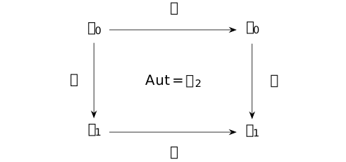
At \(a=b\), put \(z_j=(a,a,m,R_j)\). There are two objects, each with automorphism group \(C_2\times C_2\):

The generators \(s,r\) reach every displayed object; there are exactly 4 objects when \(a\ne b\) and two when \(a=b\). It follows in both directions that the coarse isomorphism classes are \((m,\{a,b\})\). The coarse orbit set forgets the isotropy just computed, as in Example [fgap-000P]. On the strict slice \((1,t,m,R_0)\), isomorphism requires the same mass and \(\{1,t\}=\{1,t'\}\), whose products give \(t=t'\). Thus reciprocal parameters are not identified there unless \(t=1\). This is a set-level groupoid, within the boundary before stacks.
Mathlib's CategoryTheory.ActionCategory constructs
the generic action category; a group action makes it a groupoid.
CategoryTheory.ActionCategory.stabilizerIsoEnd
identifies the stabilizer monoid with endomorphisms, which are invertible
in the group case. MulAction.orbitRel and
MulAction.stabilizer provide the generic coarse relation
and subgroup. DihedralGroup.card gives 8 elements
at \(n=4\), and DihedralGroup.center_eq_closure_of_even_ne_two
gives the central half-turn. In its constructor convention our
\(r^ks\) corresponds to \(\texttt {sr}(-k)\), while \(r^k\)
corresponds to \(\texttt {r}(k)\). These declarations support the
group constructions; the particular parameter action, signed incidence
and stabilizer intersections are the calculations above.
Proposition 17.2. Scalar descent and transport of Gaussian observables [fdip-000Y]AGENTDRAFTED
- October 18, 2026
Proposition 17.2. Scalar descent and transport of Gaussian observables [fdip-000Y]AGENTDRAFTED
- October 18, 2026
On the enriched four-cycle groupoid, the trace ratio, with the cycle values, is a scalar on isomorphism classes, while covariance and effective precision are transported operators on their specified field spaces. For \(x=(a,b,m,R)\) write \(C_x=Q_x^{-1}\). If \(g:x\to y\), then \[\begin {aligned} C_y&=P_gC_xP_g^T,\\ (P_g)_*\mu _{Q_x}&=\mu _{Q_y},\\ \langle F\rangle _{Q_y}&=\langle F\circ P_g\rangle _{Q_x}. \end {aligned}\] The last identity holds for Borel \(F\in L^1(\mu _{Q_y})\); integrability is equivalent to that of \(F\circ P_g\) in the source law. These statements use the inverse-precision covariance and Gaussian transport, including their normalization.
Proof.
- October 18, 2026
Proof.
- October 18, 2026
The groupoid construction proves \(Q_y=P_gQ_xP_g^T\) and \(P_g^{-1}=P_g^T\). Inverting gives the covariance equation. The normalized density in dimension \(4\) is \[d\mu _Q(\phi )=\frac {\sqrt {\det Q}}{(2\pi )^2} e^{-\phi ^TQ\phi /2}\,d\phi .\] Set \(\psi =P_g\phi \). The absolute Jacobian is one. The exponent is now \(-\psi ^TQ_y\psi /2\). Also \(\det Q_y=\det Q_x\), proving the pushforward identity. Apply the same substitution to \(|F|\) first, then to the positive and negative parts when finite, to prove the expectation statement. Transport composes because \(P_{kg}=P_kP_g\).
Transport does not imply equality of labeled arrays. At \((a,b,m)=(1,2,1)\), the spectral covariance formula gives \[\begin {aligned} (C_x)_{01} &=\tfrac 14(1-\tfrac 13+\tfrac 15-\tfrac 17)\\ &=\tfrac {19}{105},\\ (P_rC_xP_r^T)_{01} &=\tfrac 14(1+\tfrac 13-\tfrac 15-\tfrac 17)\\ &=\tfrac {26}{105}. \end {aligned}\] The second entry is the old \((3,0)\) entry. The observable's coordinate labels must move with the field to preserve its expectation.
Let \(D=V\setminus R\). In retained/eliminated coordinates write \[\begin {aligned} Q_x&=\begin {pmatrix}A&H\\H^T&C_D\end {pmatrix},\\ S_R(x)&=A-HC_D^{-1}H^T. \end {aligned}\] This Schur complement is the positive precision of the marginal. The restrictions of \(g\) give permutation isometries \(P_R:\mathbb R^R\to \mathbb R^{gR}\) and \(P_D:\mathbb R^D\to \mathbb R^{gD}\). Then \[\begin {aligned} S_{gR}(y)&=P_RS_R(x)P_R^T,\\ S_{gR}(y)^{-1}&=P_RS_R(x)^{-1}P_R^T,\\ \pi _{gR}P_g&=P_R\pi _R. \end {aligned}\] Thus the marginal laws are compatible on the changing retained spaces.
Proof.
- October 18, 2026
Proof.
- October 18, 2026
The transformed blocks are \[\begin {aligned} A'&=P_RAP_R^T,\\ H'&=P_RHP_D^T,\\ C_D'&=P_DC_DP_D^T. \end {aligned}\] Substitution, using \(P_D^TP_D=I\), gives \[\begin {aligned} S_{gR}(y)&=A'-H'(C_D')^{-1}(H')^T\\ &=P_R(A-HC_D^{-1}H^T)P_R^T. \end {aligned}\] Inversion proves the covariance equation. The projection identity holds on each vertex coordinate vector. Consequently \[\begin {aligned} (P_R)_*\mu _{S_R(x)} &=(P_R\pi _R)_*\mu _{Q_x}\\ &=(\pi _{gR}P_g)_*\mu _{Q_x}\\ &=(\pi _{gR})_*\mu _{Q_y} =\mu _{S_{gR}(y)}. \end {aligned}\] Restrictions of composable permutations compose on these spaces, so the identities are compatible with composition.
For either opposite pair in ascending coordinate order, put \(d=a+b+m^2\). Direct block multiplication gives \[\begin {aligned} A=C_D&=dI_2,\\ H&=-\begin {pmatrix}a&b\\b&a\end {pmatrix},\\ S_R(x)&=\begin {pmatrix}\alpha &-\beta \\-\beta &\alpha \end {pmatrix},\\ \alpha &=d-\frac {a^2+b^2}{d},\\ \beta &=\frac {2ab}{d}. \end {aligned}\] This particular two-by-two array is unchanged by swapping weights or retained coordinates. That special equality does not make general operator assignments scalar invariants; the full covariance entries above already differ.
For the nonzero positive semidefinite \(L_x\), define \[\mathcal R(x)=\frac {\operatorname {tr}(L_x^2)} {\bigl (\operatorname {tr}L_x\bigr )^2}.\] Then \(\mathcal R(gx)=\mathcal R(x)\), and \[\mathcal R(a,b)=\frac {a^2+ab+b^2}{2(a+b)^2}.\] This scalar descends to the coarse orbit set but does not classify the enriched objects.
Proof.
- October 18, 2026
Proof.
- October 18, 2026
Trace cyclicity gives \(\operatorname {tr}(P_gMP_g^T)=\operatorname {tr}M\). Also \(L_{gx}^2=P_gL_x^2P_g^T\); hence both traces are preserved. For the explicit value, the 4 orthonormal vectors \(u_0,u_1,u_2,u_3\) from Example 7.19 remain eigenvectors after replacing weights \((1,t)\) by \((a,b)\), with eigenvalues \(0,2a,2b,2a+2b\). Substituting the alternating entries of \(L_x\) verifies each eigenvector equation. Therefore \[\begin {aligned} \operatorname {tr}L_x&=4(a+b)>0,\\ \operatorname {tr}(L_x^2)&=8(a^2+ab+b^2). \end {aligned}\] These spectral trace identities use [boyd2004convex, Appendix A.5.2, pp. 646-647]. The positive denominator justifies the division. In particular \[\begin {aligned} \mathcal R(1,1)&=\frac 38,\\ \mathcal R(1,2)&=\frac 7{18},\\ \frac 7{18}-\frac 38&=\frac 1{72}. \end {aligned}\] The ratio ignores \(m\), so backgrounds of different masses have the same value. It also satisfies \(\mathcal R(1,t)=\mathcal R(1,1/t)\), although the strict slice objects are inequivalent for \(t\ne 1\) by Example 17.1.
Now forget mass, state and partition and admit positive scaling of the Laplacian, as in the broader comparison: \[L'=cP_gLP_g^T,\qquad c>0.\] The numerator of \(\mathcal R\) gains \(c^2\), while its denominator gains the same factor. Thus the ratio is invariant under this different relation. A weight-swapping relabeling followed by \(c=1/t\) sends \(L(1,t)\) to \(L(1,1/t)\). Reciprocal parameters are identified in this reduced problem only; no scale arrow has been added to the original Gaussian groupoid. At fixed mass, \(cL+m^2I\ne cQ\) for \(c\ne 1\). If one instead rescales the entire precision to \(cQ\), then \[\begin {aligned} (cQ)^{-1}&=c^{-1}Q^{-1},\\ cA-(cH)(cC_D)^{-1}(cH)^T&=cS_R. \end {aligned}\] Raw covariance and effective precision therefore are not scale invariants. Any normalized operator ratio would need its own definition and scaling proof.
Mathlib's Matrix.trace_units_conj and
Matrix.trace_smul support the trace conjugacy and scaling
identities. Matrix.reindexLinearEquiv and
Matrix.reindexRingEquiv supply coordinate infrastructure.
TauCeti's
TauCeti.Probability.map_affine_multivariateGaussian
allows positive semidefinite covariance and an arbitrary rectangular
linear map. Set its mean and translation to zero, its covariance
to \(Q_x^{-1}\), and its linear map to \(P_g\) or \(\pi _R\).
The precision-density identification and the Schur and groupoid
computations above remain separate obligations.
Example 17.3. Quadratic isometry forgets the reference pairing and projection [fdip-000Z]AGENTDRAFTED
- October 18, 2026
Example 17.3. Quadratic isometry forgets the reference pairing and projection [fdip-000Z]AGENTDRAFTED
- October 18, 2026
The enriched classification changes if one keeps only a positive quadratic form and permits every linear isometry. Any two positive symmetric matrices \(Q_1,Q_2\) of the same size define isometric quadratic spaces, even when their counting-relative spectra and retained observables differ.
[boyd2004convex, Appendix A.5.2, pp. 646-647] gives the symmetric spectral decomposition and positive square root used below to construct the isometry.
For \(Q=O\operatorname {diag}(\lambda _i)O^T\), with \(O\) orthogonal and every \(\lambda _i>0\), define \[\begin {aligned} Q^{1/2}&=O\operatorname {diag}(\sqrt {\lambda _i})O^T,\\ A=Q^{-1/2}&=O\operatorname {diag}(\lambda _i^{-1/2})O^T. \end {aligned}\] Direct multiplication gives \(A^TQA=I\). More generally, \[\begin {aligned} T&=Q_2^{-1/2}Q_1^{1/2},\\ T^TQ_2T &=Q_1^{1/2}Q_2^{-1/2}Q_2Q_2^{-1/2}Q_1^{1/2}\\ &=Q_1. \end {aligned}\] The map \(T\) is invertible. This calculation does not require \(Q_1Q_2=Q_2Q_1\). Thus positive quadratic forms have one linear-isometry class in each fixed dimension.
The reference pairing changes under the same substitution \(\phi =Az\): its matrix becomes \[H'=A^TIA=Q^{-1},\] while the action form has matrix \(I\). If that transported pairing is retained, its relative operator is \((H')^{-1}I=Q\), preserving the original spectrum. In general simultaneous transport of a positive reference pairing \(H\) and an action form \(Q\) gives \[\begin {aligned} H'&=A^THA,\qquad Q'=A^TQA,\\ (H')^{-1}Q'&=A^{-1}(H^{-1}Q)A. \end {aligned}\] Similarity preserves the spectrum. Replacing \(H'\) by \(I\) after normalizing \(Q\) discards this data; it is not simultaneous transport of the pair.
For the four-cycle with \(a=m=1\), compare \(b=1\) and \(b=2\). The spectral calculation gives respectively \[\begin {aligned} \operatorname {spec}(Q_1)&=\{1,3,3,5\},\\ \operatorname {spec}(Q_2)&=\{1,3,5,7\}. \end {aligned}\] These forms are linearly isometric by \(T\), but cannot be conjugate by a counting-orthogonal map, since their spectra differ. In particular they are not compatible relabelings. Their trace ratios also differ by \(1/72\).
The same isometry gives a concrete obstruction to the retained projection, even though it preserves the named half-turn. In the common orthonormal spectral basis \(u_0,u_1,u_2,u_3\), the matrix of \(T\) is \[\operatorname {diag}\bigl (1,1,\sqrt {3/5},\sqrt {5/7}\bigr ).\] The half-turn is diagonal in this basis as well, so \(T\rho (h)=\rho (h)T\). Returning to vertex coordinates gives \[T_{01}=\frac {\sqrt {3/5}-\sqrt {5/7}}4\ne 0,\] because \(3/5\ne 5/7\). For \(R=R_0\), one has \(\pi _R\delta _1=0\), whereas the zeroth component of \(\pi _RT\delta _1\) is nonzero. Hence no linear map \(T_R\) can satisfy \(\pi _RT=T_R\pi _R\). Also \(T^TT\) has eigenvalues \(1,1,3/5,5/7\), so \(T\) fails to preserve the counting pairing. These are separate failures of the enriched-arrow conditions.
A Jacobian magnitude different from one does not obstruct normalized Gaussian transport. If \(T^TQ_2T=Q_1\), then \[\det Q_1=(\det T)^2\det Q_2.\] For \(y=T\phi \), the exponent in the normalized density becomes \(-y^TQ_2y/2\); its coefficient after the reference change of variables is \[\frac {\sqrt {\det Q_1}}{(2\pi )^{n/2}|\det T|} =\frac {\sqrt {\det Q_2}}{(2\pi )^{n/2}}.\] Therefore \(T_*\mu _{Q_1}=\mu _{Q_2}\). Equivalently, \(Q_2^{-1}=TQ_1^{-1}T^T\) is the covariance transport law. For \(A=Q^{-1/2}\), the Jacobian magnitude \(|\det A|=(\det Q)^{-1/2}\) is exactly absorbed by normalization, even when it differs from one. The loss is the discarded pairing, carrier and retained projection, not a failure of normalized probability transport.
TauCeti's
Matrix.PosDef.exists_generalLinearGroup_mul_transpose_eq
provides an invertible factor \(C\) with \(Q=CC^T\) for a real
positive-definite matrix on a finite index set. For a bare witness
of that conclusion the normalizer is \(C^{-T}\), since
\[(C^{-T})^TQ C^{-T}=C^{-1}CC^TC^{-T}=I.\]
The theorem's proof chooses the symmetric positive square root,
but its existential conclusion does not assert symmetry of \(C\).
One therefore cannot infer that \(C^{-1}\) is the normalizer
from the factorization alone. Its separate
TauCeti.Probability.map_affine_multivariateGaussian
supports Gaussian transport in covariance parameters, after the
precision-density identification. Neither declaration supplies the
enriched classification or projection obstruction.
By Clifford functoriality, an isometry of these configuration forms also induces an algebra isomorphism. Since the positive forms already lie in one isometry class, keeping only the abstract quadratic space, or its isometry-functorial Clifford algebra, cannot recover the discarded reference pairing, carrier and projection. This argument does not infer a quadratic isometry from an arbitrary Clifford-algebra isomorphism. Retaining the enriched objects and their specified relabeling arrows prevents the demonstrated collapse; it supplies no continuum or physical selection map.
18. Arithmetic families [fdip-001D]AGENTDRAFTED
- October 20, 2026
18. Arithmetic families [fdip-001D]AGENTDRAFTED
- October 20, 2026
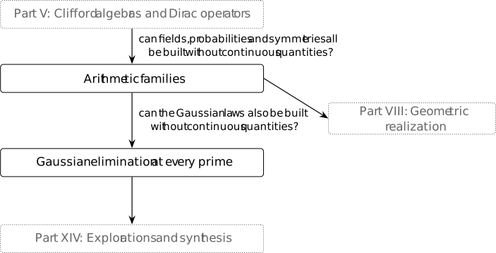
Which constructions survive if field values use finite arithmetic instead of the real numbers? For each prime \(p\), the finite field \(\mathbb F_p\) gives such a value system. Comparing it with a real model requires a specified arithmetic family and control of denominators. The four-cycle coefficients give an arithmetic family over \(\mathbb Z[1/2,t]\). Scalar extension organizes its Clifford algebras, while the form, elimination map and observable ratio each impose their own domain. Bad fibers distinguish those domains concretely. This base excludes characteristic two, where the earlier half-turn example shows how an algebra can survive while its sector decomposition changes.
The rational comparison uses Gaussian elimination and the reference pairing and trace conventions. It distinguishes the information in a quadratic center character from the independently defined trace observable. These arithmetic families also supply the fiber-constancy criterion used by the realization comparison.
With rational positive-definite precision in counting coordinates, the Gaussian covariance \(Q^{-1}\) is rational, although its normalized real law still uses real integration. Which moment and partition-function identities have arithmetic counterparts? The prime-by-prime Gaussian chapter gives the moment rule over a ring. The finite-field partition functions are not constructed there.
Example 18.1. An arithmetic family for the alternating four-cycle [fdip-000U]AGENTDRAFTED
- October 18, 2026
Example 18.1. An arithmetic family for the alternating four-cycle [fdip-000U]AGENTDRAFTED
- October 18, 2026
The configuration form has polynomial coefficients when the mass is fixed by \(m^2=1\). Keeping the weight \(t\) as a variable records which specializations preserve the form, its half-turn, and the operations on it. Put \(A_0=\mathbb Z[1/2,t]\) and \(s=t+2\). In the coordinate basis \(\delta _0,\ldots ,\delta _3\), set \[Q(t)=\begin {pmatrix} s&-1&0&-t\\ -1&s&-t&0\\ 0&-t&s&-1\\ -t&0&-1&s \end {pmatrix},\] \[\begin {aligned} q(x)&=x^TQ(t)x,\\ b(x,y)&=x^TQ(t)y. \end {aligned}\] Thus \(q\) is twice the earlier quadratic action. Its half-polar form is \(b\); its full polar form has matrix \(2Q\): \[q(x+y)-q(x)-q(y)=2b(x,y).\] These conventions also apply after changing the coefficient ring.
Let \(H\) have the 4 unnormalized columns \[H=\begin {pmatrix} 1&1&1&1\\ 1&-1&1&-1\\ 1&-1&-1&1\\ 1&1&-1&-1 \end {pmatrix}.\] They are neither the coordinate vectors \(\delta _i\) nor the normalized real spectral vectors \(u_a\) of the cycle spectral calculation. Direct multiplication gives \[\begin {aligned} H^TH&=4I,\\ QH&=H\operatorname {diag}(1,3,2t+1,2t+3). \end {aligned}\] Since \(2\) is a unit in \(A_0\), \(H^{-1}=H^T/4\). Similarity therefore gives \[\Delta :=\det Q=3(2t+1)(2t+3).\] The congruence formula retains a factor 4: \[H^TQH=4\operatorname {diag}(1,3,2t+1,2t+3).\] These are polynomial matrix identities, independent of any order or positivity on the coefficient ring.
The nondegenerate arithmetic base is \[R_q=A_0[\Delta ^{-1}],\qquad X_q=\operatorname {Spec}R_q,\] with quadratic module \((R_q^4,q)\). Here \(A[g^{-1}]\) denotes localization of a commutative ring \(A\) by the powers of \(g\). The spectrum \(\operatorname {Spec}A\) has prime ideals as points; its standard open \[D_{\operatorname {Spec}A}(g) =\{\mathfrak p:g\notin \mathfrak p\}\] has regular functions \(A[g^{-1}]\). The structure sheaf given by these rings and their restriction maps makes the spectrum an affine scheme, in the sense of [stacks2017stacks, Section 26.5], Tag 01HR.
Every factor of the unit product \(\Delta \) is a unit in \(R_q\): an inverse for a factor is the product of the other factors times \(\Delta ^{-1}\). The displayed similarity then makes \(Q\) invertible. Both \(Q\) and \(2Q\) identify \(R_q^4\) with its dual. This localization selects nondegenerate forms; the Clifford quotient exists over \(A_0\) even before it is made. Inverting \(2\) separately excludes characteristic two, although \(\Delta \equiv 1\pmod 2\). Inverting \(\Delta \) removes characteristic three entirely. In any residue field of characteristic other than two or three, the excluded parameters are \(-1/2\) and \(-3/2\); they are distinct because their difference is one.
For example, evaluation at \(t=1\) gives \(\det Q=45\). It is admissible over \(\mathbb Q\) and over \(\mathbb F_{11}\), but not over \(\mathbb F_5\). An arithmetic family therefore retains information that a single real matrix does not.
The same half-turn \[P(x_0,x_1,x_2,x_3)=(x_2,x_3,x_0,x_1)\] satisfies \(P^2=I\) and \(P^TQP=Q\): shifting both indices by two preserves each entry of \(Q\). By the universal property, the assignment \[\iota _q(x)\longmapsto \iota _q(Px)\] extends to an algebra endomorphism of \(\operatorname {Cl}_{R_q}(q)\). Its square fixes scalars and all vector generators, hence is the identity. It defines a \(C_2\) action by automorphisms. The coordinate basis, reference pairing \(x^Ty\), and retained partition remain additional supplied data.
Retain coordinates \((0,2)\) and eliminate \((1,3)\) as in the four-cycle Schur calculation. To distinguish its denominator from that of the trace ratio on its unit domain, put \(f=t+1\) and define \[\begin {aligned} R_{\mathrm {elim}}&=R_q[s^{-1}],\\ R_{\mathrm {obs}}&=R_{\mathrm {elim}}[f^{-1}],\\ X_{\mathrm {elim}}&=\operatorname {Spec}R_{\mathrm {elim}},\\ X_{\mathrm {obs}}&=\operatorname {Spec}R_{\mathrm {obs}},\\ U_R&=D_{X_q}(f). \end {aligned}\] The open immersions identify \[\begin {aligned} X_{\mathrm {elim}}&=D_{X_q}(s),\\ X_{\mathrm {obs}}&=D_{X_{\mathrm {elim}}}(f) =D_{X_q}(sf),\\ X_{\mathrm {obs}}&=X_{\mathrm {elim}}\cap U_R. \end {aligned}\] The independent ratio locus \(U_R\) is not identified with \(X_{\mathrm {obs}}\); at \(t=-2\), the ratio exists while the selected elimination fails.

All 4 arrows are inclusions of open subschemes. The square
commutes and its upper-left open is the intersection of the
other two opens inside \(X_q\). The localization homeomorphism is
[stacks2017stacks, Lemma 10.17.6], Tag 00E4.
The structure-sheaf construction in
[stacks2017stacks, Section 26.5], Tag 01HR
upgrades it to an open immersion: on a standard open inside
\(D(g)\), successive localization gives the same ring and
restriction map on either side. These identifications agree on
intersections, so the structure sheaves agree. Mathlib's
AlgebraicGeometry.Scheme.isOpenImmersion_SpecMap_localizationAway
and AlgebraicGeometry.Scheme.Hom.opensRange_localizationAway
give this generic map and its exact ambient image. The
determinant and the particular family above are the direct
calculations made here.
Theorem 18.2. Clifford algebras under scalar extension [fdip-000V]
L∃∀NAGENTDRAFTED
- October 18, 2026
Theorem 18.2. Clifford algebras under scalar extension [fdip-000V]
L∃∀NAGENTDRAFTED
- October 18, 2026
Let \(R\) be a commutative ring in which \(2\) is a unit, \(M\) any \(R\)-module with quadratic form \(q\), and \(A\) any commutative \(R\)-algebra. Extend the symmetric half-polar form \[b(v,w)=\frac {q(v+w)-q(v)-q(w)}2\] to \(M_A=A\otimes _R M\), and let \(q_A\) be its diagonal. Thus \[q_A(a\otimes v)=a^2q(v),\] where \(q(v)\) on the right is mapped into \(A\). There is a canonical \(A\)-algebra isomorphism \[\begin {aligned} \beta _A:A\otimes _R\operatorname {Cl}_R(q) &\longrightarrow \operatorname {Cl}_A(q_A),\\ \beta _A(a\otimes \iota _q(v)) &=a\,\iota _{q_A}(1\otimes v). \end {aligned}\] No flatness, nondegeneracy, finite generation, or injectivity of \(R\to A\) is required. This extends the displayed field case of scalar extension to the declared commutative rings, using the same universal property.
Proof.
- October 18, 2026
Proof.
- October 18, 2026
The \(R\)-linear map \(v\mapsto \iota _{q_A}(1\otimes v)\) has square \(q(v)1\), so the universal property extends it to an \(R\)-algebra map out of \(\operatorname {Cl}_R(q)\). Central \(A\)-scalars then extend it to \(\beta _A\). The algebra structure on the tensor product uses \[(a\otimes c)(a'\otimes c')=aa'\otimes cc'.\] It is well-defined because the \(R\)-scalars are central.
Conversely, the balanced bilinear assignment \((a,v)\mapsto a\otimes \iota _q(v)\) gives an \(A\)-linear map \[j:M_A\longrightarrow A\otimes _R\operatorname {Cl}_R(q).\] Write \(\iota =\iota _q\) and let \[\begin {aligned} B_q(v,w)&=q(v+w)\\ &\quad -q(v)-q(w)\\ &=2b(v,w) \end {aligned}\] be the full polar form. The defining square relation gives \[\iota (v)\iota (w)+\iota (w)\iota (v)=B_q(v,w)1.\] For an arbitrary finite sum \(x=\sum _i a_i\otimes v_i\), write \(w_i=\iota (v_i)\). Then \[\begin {aligned} j(x)^2 &=\sum _i a_i^2\otimes w_i^2\\ &+\sum _{i<j}a_i a_j\otimes (w_iw_j+w_jw_i)\\ &=\Bigl (\sum _i a_i^2q(v_i)\\ &\quad +\sum _{i<j}a_i a_j B_q(v_i,v_j)\Bigr )1\\ &=q_A(x)1. \end {aligned}\] Every tensor is such a finite sum; the cross terms are part of the square condition. Thus \(j\) extends to an \(A\)-algebra map in the opposite direction. Both composites fix scalars and vector generators. In the tensor-product algebra, \(a\otimes 1\) and \(1\otimes \iota (v)\) generate; in the other algebra, the vectors \(\iota _{q_A}(x)\) and scalars generate. The composites are therefore identities.
Mathlib's marked equivalence has the reverse direction,
\[\operatorname {Cl}_A(q_A)
\simeq A\otimes _R\operatorname {Cl}_R(q).\]
Its inverse is \(\beta _A\), and
CliffordAlgebra.ofBaseChange_tmul_ι
gives the displayed generator formula.
QuadraticForm.baseChange constructs \(q_A\); its
QuadraticForm.baseChange_tmul computes pure tensors.
These declarations have exactly the commutative-ring and
invertible-two hypotheses above. The marker concerns the
generic algebra equivalence, not the arithmetic domain
calculations or the sheaf multiplication below.
Scalar extension is compatible with a further commutative
algebra \(A\to B\). Identify
\[\begin {aligned}
B\otimes _A(A\otimes _R M)&\longrightarrow B\otimes _R M,\\
b\otimes (a\otimes v)&\longmapsto ba\otimes v.
\end {aligned}\]
The inverse inserts \(1\) in the middle tensor factor.
Under this identification the direct and successive Clifford
maps both send \(b\otimes (a\otimes \iota _q(v))\) to
\(ba\,\iota _{q_B}(1\otimes v)\). These elements and scalars
generate, proving equality of the algebra maps. TauCeti's
QuadraticForm.baseChangeBaseChange
uses the inverse identification, from direct to successive
extension. With compatible \(R\)- and \(A\)-algebra structures
on \(B\), its
CliffordAlgebra.ofBaseChangeAux_baseChange
states the same compatibility in that direction.
For an \(R\)-linear form-preserving map \(P:M\to M\), put \(P_A(a\otimes v)=a\otimes Pv\). The two orders of applying \(\beta _A\) and the induced Clifford map both take \(a\otimes \iota _q(v)\) to \(a\,\iota _{q_A}(1\otimes Pv)\). Generation again proves equivariance. In particular the arithmetic half-turn and its \(C_2\) action commute with every allowed scalar extension.
Apply this to \(C=\operatorname {Cl}_{R_q}(q)\) on the
arithmetic base \(X_q\). Write
\(\mathcal O_{X_q}\) for its structure sheaf: regular functions
on \(D_{X_q}(g)\) form \((R_q)_g\). The
associated module sheaf \(\widetilde C\) has
\[\Gamma (D_{X_q}(g),\widetilde C)
=C_g\simeq (R_q)_g\otimes _{R_q}C.\]
Its restriction maps are the localization maps; compatible
local sections glue uniquely. This construction and the
standard-open formula are
[stacks2017stacks, Section 26.5 and Lemma 26.5.4], Tag 01HR.
Mathlib's AlgebraicGeometry.tilde, with its
standard-open localized-module instance, supplies the underlying
module sheaf. It does not by itself give the algebra structure.
Multiplication and unit on a standard open are \[\frac {c}{g^m}\frac {d}{g^n} =\frac {cd}{g^{m+n}},\qquad 1=\frac 11.\] The denominators are central, so these operations are well-defined even though \(C\) need not be commutative. Restriction maps preserve them. On an arbitrary open, cover by standard opens and multiply the restrictions of two sections. The products agree on overlaps, so the module-sheaf axiom glues them uniquely; the same argument glues the unit. Associativity, additivity, the unit law and central \(\mathcal O_{X_q}\) action hold locally and hence globally. Thus \(\widetilde C\) is a sheaf of unital associative \(\mathcal O_{X_q}\)-algebras. No spectrum of the noncommutative algebra \(C\) is taken.
The isomorphisms \(\beta _{(R_q)_g}\) identify these standard-open sections with \[\operatorname {Cl}_{(R_q)_g}(q_g).\] Scalar-tower compatibility makes the identifications commute with restrictions. This constructs the Clifford algebra sheaf of \(\mathcal O_{X_q}^4\) with matrix \(Q\). The half-turn acts on every localization by the same generator formula and commutes with restrictions, giving a \(C_2\) action on the sheaf. Restricting to \(X_{\mathrm {elim}}\) or \(X_{\mathrm {obs}}\) uses exactly these base-change maps.
At the real specialization \(t=1\), put \(q_1(x)=x^TQ(1)x\) and let \(c_i=\iota _{q_1}(\delta _i)\) with the coordinate notation of the configuration Clifford algebra. Then \[c_i^2=3\,1,\qquad c_ic_j+c_jc_i=2Q(1)_{ij}\,1.\] The map \(\beta _{\mathbb R}\) identifies these relations with \(\mathbb R\otimes _{R_q}C\); direct evaluation or evaluation through either localization gives the same algebra and action. This evaluation is not injective: it kills the nonzero element \(t-1\) of \(R_q\). The isomorphism requires no injectivity. The effective rank-two form has its own Clifford algebra on \(X_{\mathrm {elim}}\); it is separate from this rank-4 construction.
Proposition 18.3. Different domains for the form, elimination and trace ratio [fdip-000W]AGENTDRAFTED
- October 18, 2026
Proposition 18.3. Different domains for the form, elimination and trace ratio [fdip-000W]AGENTDRAFTED
- October 18, 2026
On the arithmetic family, a nondegenerate full form need not permit a chosen elimination, and an invertible effective form need not give a regular trace ratio. With \(s=t+2\), \(f=t+1\) and \(\Delta =3(2t+1)(2t+3)\), the exact regular loci in \(X_q\) are \[\begin {aligned} \text {Schur matrix:}&\quad X_{\mathrm {elim}}=D_{X_q}(s),\\ \text {trace ratio:}&\quad U_R=D_{X_q}(f). \end {aligned}\] Their common domain is \(X_{\mathrm {obs}}=D_{X_q}(sf)\). These claims follow from the calculations below, extending the real Schur example and trace-ratio calculation over the declared rings. The intrinsic trace ratio requires a unit trace: \(\operatorname {tr}L=4f\) is a unit exactly when \(f\) is, since \(2\) is already inverted.
Proof.
- October 18, 2026
Proof.
- October 18, 2026
Order coordinates by retained \((0,2)\) and eliminated \((1,3)\). The diagonal blocks of \(Q\) are \(A=C_{\mathrm {block}}=sI_2\), and the off-diagonal block is \[B=\begin {pmatrix}-1&-t\\-t&-1\end {pmatrix}.\] On \(R_{\mathrm {elim}}\), the Schur matrix is \[\begin {aligned} S&=A-BC_{\mathrm {block}}^{-1}B^T\\ &=\frac 1s\begin {pmatrix}4t+3&-2t\\-2t&4t+3\end {pmatrix}. \end {aligned}\] Indeed \(BB^T\) has diagonal \(1+t^2\) and off-diagonal \(2t\), and \(s^2-(1+t^2)=4t+3\). Moreover \[\det S=\frac {(4t+3)^2-4t^2}{s^2} =\frac {\Delta }{s^2},\] a unit in \(R_{\mathrm {elim}}\). On \(R_{\mathrm {elim}}^2\), define \(q_{\mathrm {eff}}(y)=y^TSy\); its half-polar matrix is \(S\). Thus both \(q\) and \(q_{\mathrm {eff}}\) are nondegenerate on this open. On the positive real locus, \(q_{\mathrm {eff}}/2\) is the quadratic part of the effective action; the Gaussian normalization constant is additional.
The domain \(R_q\) embeds in its fraction field, so these entries can be tested in each local ring. If a prime \(\mathfrak p\) contains \(s\), the off-diagonal numerator \(-2t\) is congruent to \(4\) modulo \(\mathfrak p\) and is a unit in \((R_q)_{\mathfrak p}\). If \((-2t)/s\) were regular there, multiplication by \(s\) would equate an element of the maximal ideal with a unit. This is impossible. On \(D_{X_q}(s)\) every entry is regular. Hence this is the exact regular locus of the displayed Schur matrix.
For \(L=Q-I\), the diagonalization in Example 18.1 gives eigenvalues \(0,2,2t,2t+2\). Therefore \[\begin {aligned} \operatorname {tr}L&=4(t+1),\\ \operatorname {tr}(L^2)&=8(t^2+t+1),\\ R(t)&=\frac {\operatorname {tr}(L^2)}{(\operatorname {tr}L)^2} =\frac {t^2+t+1}{2(t+1)^2}. \end {aligned}\] The numerator is \(f^2-f+1\). At every prime containing \(f\), it has residue \(1\), so is a unit in the local ring. Regularity of \(R\) there would make \[2f^2R=f^2-f+1\] an equality of an element of the maximal ideal and a unit, again impossible. Where \(f\) is invertible the formula is regular. Thus the exact ratio locus is \(U_R\), and its intersection with \(X_{\mathrm {elim}}\) is \(X_{\mathrm {obs}}\). The interpretation of these localizations as regular functions is [stacks2017stacks, Lemma 26.5.4], Tag 01HR.
The half-turn restricts to \(J=\left (\begin {smallmatrix}0&1\\1&0\end {smallmatrix}\right )\) on both coordinate blocks. The equal diagonal and equal off-diagonal entries of \(S\) give \(J^TSJ=S\). Retained projection \(\pi \) satisfies \(\pi P=J\pi \), but is not an isometry: \(q(\delta _1)=s\) is a unit on \(R_{\mathrm {elim}}\), whereas \(\pi \delta _1=0\). Thus Clifford functoriality supplies no map induced by this projection. The effective rank-two Clifford algebra and the full rank-4 algebra are different constructions.
Three rational specializations separate the domains:
- At \(t=-2\), \(\det Q=9\) and \(R=3/2\), but \(C_{\mathrm {block}}=0\). This point belongs to \(U_R\) inside \(X_q\) and lies outside \(X_{\mathrm {elim}}\).
- At \(t=-1\), \(\det Q=-3\), \(C_{\mathrm {block}}=I_2\), and \[\begin {aligned} S&=\begin {pmatrix}-1&2\\2&-1\end {pmatrix},\\ \det S&=-3. \end {aligned}\] This point belongs to \(X_{\mathrm {elim}}\), but the trace ratio has a pole, so it lies outside \(X_{\mathrm {obs}}\).
- At \(t=1\), \(\det Q=45\), \(C_{\mathrm {block}}=3I_2\), and \[\begin {aligned} S&=\frac 13\begin {pmatrix}7&-2\\-2&7\end {pmatrix},\\ \det S&=5,\qquad R=\frac 38. \end {aligned}\] This point belongs to \(X_{\mathrm {obs}}\).
For real \(t=\tau \), the matrix \(H/2\) is orthogonal, and the 4 eigenvalues of \(Q(\tau )\) are \(1,3,2\tau +1,2\tau +3\). They are all positive exactly when \(\tau >-1/2\). The running weighted graph assumes the smaller domain \(\tau >0\). Each such evaluation sends \(2,\Delta ,s,f\) to nonzero reals and extends uniquely to \[R_{\mathrm {obs}}\longrightarrow \mathbb R,\qquad t\longmapsto \tau .\] It gives \(\operatorname {Spec}\mathbb R\to X_{\mathrm {obs}}\) and recovers \(Q(\tau ),S(\tau ),P,J,R(\tau )\). The Clifford base-change isomorphism transports their full-form algebra and symmetry; it does not require evaluation to be injective. Gaussian integration and the normalized marginal apply on this positive real locus. Algebraic invertibility alone gives neither positivity nor a probability measure over the arithmetic base.
This family retains a parameter, residue characteristics, and distinct regularity domains. It does not select a unique arithmetic realization. For example, at \(t=1\) modulo \(11\), \(\Delta =45\), \(s=3\), and \(f=2\) are all nonzero. The point therefore lies in \(X_{\mathrm {obs}}\), but disappears after further inverting \(11\). Every real specialization survives that extra inversion. Thus the same real family admits different arithmetic opens. The construction predicts neither a real parameter nor a physical observable from arithmetic alone; an L-value comparison needs additional structure.
Definition 18.4. Enriched rational objects and relative precision [fdip-0041]AGENTDRAFTED
- October 31, 2026
Definition 18.4. Enriched rational objects and relative precision [fdip-0041]AGENTDRAFTED
- October 31, 2026
The arithmetic family has both a quadratic form and an operator relative to a specified pairing. To separate the information they retain, an enriched rational object consists of data \[\mathcal B=(V,g_0,q,m^2,V_{\mathrm {ret}},V_{\mathrm {el}}).\] Here \(V\) has dimension \(4\) over \(\mathbb Q\), \(g_0\) is a rational positive definite symmetric pairing, and \(q\) is a rational quadratic form whose half-polar pairing \[b_q(v,w)=\frac {q(v+w)-q(v)-q(w)}2\] is positive definite after extension to \(\mathbb R\). Fix \(m^2\in \mathbb Q_{>0}\) and a \(g_0\)-orthogonal splitting \(V=V_{\mathrm {ret}}\perp V_{\mathrm {el}}\) into two-dimensional summands. This is a rational linear analogue of the supplied pairing, mass and splitting in the enriched background data; no graph realization is assumed. These are additional data, not consequences of \(q\).
The relative precision is the unique operator \(Q:V\to V\) satisfying \[g_0(v,Qw)=b_q(v,w).\] It is the relative operator for these two pairings: rational, \(g_0\)-self-adjoint and positive definite. Define \[\begin {aligned} L_{\mathrm {rel}}&=Q-m^2I,\\ R(\mathcal B)&=\frac {\operatorname {tr}(L_{\mathrm {rel}}^2)} {\bigl (\operatorname {tr}L_{\mathrm {rel}}\bigr )^2}. \end {aligned}\] Restrict these objects to \(L_{\mathrm {rel}}\geq 0\) and \(\operatorname {tr}L_{\mathrm {rel}}\ne 0\). This is the trace ratio on its stated domain. The real Gaussian uses action \(q/2\), the volume induced by \(g_0\), and the normalized law \(\mu _Q\). Neither the factor \(1/2\) in the action nor the reference volume changes the convention \(\iota _q(v)^2=q(v)1\) of the configuration Clifford algebra.
An arrow \(T:\mathcal B\to \mathcal B'\) is a rational linear isomorphism preserving \(g_0,q,m^2\) and carrying each specified summand to its namesake. Preservation of the two pairings gives \(g'_0(Tv,Q'Tw)=g'_0(Tv,TQw)\) for all \(v,w\), whence \[Q'T=TQ,\qquad L'_{\mathrm {rel}}T=TL_{\mathrm {rel}}.\] Trace conjugacy proves \(R(\mathcal B')=R(\mathcal B)\). Identity, inverse and composition preserve these conditions, so the objects and arrows form a groupoid.
Definition 18.5. The quadratic center character [fdip-0049]AGENTDRAFTED
- October 31, 2026
Definition 18.5. The quadratic center character [fdip-0049]AGENTDRAFTED
- October 31, 2026
Let \(q\) be a nondegenerate rational quadratic form of rank 4,
with half-polar pairing \(b_q\). In particular, forgetting the extra
data of an enriched rational object supplies such a form.
Its
even Clifford algebra has quadratic center
\[E_q=Z(\operatorname {Cl}^+(q))
\simeq \mathbb Q[z]/(z^2-d),\]
where \(d\) represents the signed discriminant class
\(\delta (q)\in \mathbb Q^\times /(\mathbb Q^\times )^2\).
In rank 4 this is the determinant class of \(b_q\).
This uses exactly the field/rank-4 center statement and
proof of the discriminant center, without its
subsequent Spin identifications. For an enriched object, in any common
rational basis,
\[\det (b_q)=\det (g_0)\det (Q).\]
Each pairing determinant changes by a square under a basis
change. Thus \(\det Q\) alone does not supply \(\delta (q)\)
unless the reference-pairing determinant class is also known.
TauCeti's CliffordAlgebra.adjoinRootEquivCenterEven
gives the generic center identification from a nonempty even
orthogonal spanning list of nonisotropic vectors over a field
of characteristic different from two. It supplies this algebraic
step, not the character or trace-observable construction.
Fix an algebraic closure \(\overline {\mathbb Q}\).
The quadratic center character is the Galois character
\[\begin {aligned}
\chi _q:G_{\mathbb Q}&\longrightarrow \{1,-1\},\\
\sigma &\longmapsto \frac {\sigma (\sqrt d)}{\sqrt d},
\end {aligned}\]
where \(G_{\mathbb Q}=\operatorname {Gal}(\overline {\mathbb Q}/\mathbb Q)\).
The value is independent of the sign of the root and of
multiplying \(d\) by a rational square. If \(d\) is a square,
\(E_q\simeq \mathbb Q\times \mathbb Q\) and \(\chi _q\) is trivial.
Otherwise the center is the field \(\mathbb Q(\sqrt d)\) and
\(\chi _q\) is its quadratic character. The corresponding algebraic
dichotomy is formalized by
CliffordAlgebra.nonempty_center_even_algEquiv_prod_iff_isSquare_discriminant
and
CliffordAlgebra.isField_center_even_iff_not_isSquare_discriminant,
with the same field, characteristic and orthogonal-list hypotheses
as the center identification above. The cyclotomic description of the
character is given by Brian Conrad in
[conradQuadraticCharacters, Section 1, p. 1].
The diagram records two constructions on enriched objects. Its left downward arrow is the independently defined trace ratio; no arrow from \(\chi _q\) to \(R\) is asserted. A quadratic isometry induces an even Clifford algebra isomorphism, hence a center isomorphism and the same character.

For a nonsquare class, let \(d_0\) be its squarefree integer
representative and put \(D=d_0\) if \(d_0\equiv 1\pmod 4\),
and \(D=4d_0\) otherwise. The primitive Dirichlet representative
is \(\chi _D(n)=(D/n)\), with Kronecker-symbol convention and
value zero when \(\gcd (n,|D|)>1\); its conductor is \(|D|\).
For the split class use the trivial character of conductor one.
These conventions agree with Brian Conrad's
[conradQuadraticCharacters, Sections 1 and 3, especially Theorem 3.4].
For an integer \(D\) satisfying Int.IsFundamentalDiscr \(D\),
TauCeti's TauCeti.Multiquadratic.fundamentalDiscriminantChar
defines the integer-valued Dirichlet character of level \(|D|\), and
TauCeti.Multiquadratic.isPrimitive_fundamentalDiscriminantChar
proves it primitive, so its conductor is \(|D|\).
These declarations supply this character/conductor step, including \(D=1\).
Fix the uncompleted convention
\[L(s,\chi _D)=\prod _{p\ \mathrm {prime}}
(1-\chi _D(p)p^{-s})^{-1}\]
for \(\operatorname {Re}s>1\), and the comparison point \(s=2\). The product converges absolutely;
no gamma or conductor factor is included. The Euler convention
is Brian Conrad's [conradQuadraticCharacters, p. 5].
The factorization criterion asks whether this
character retains enough information to recover \(R\).
Proposition 18.6. Factorization through an invariant requires fiber constancy [fdip-0042]AGENTDRAFTED
- October 30, 2026
Proposition 18.6. Factorization through an invariant requires fiber constancy [fdip-0042]AGENTDRAFTED
- October 30, 2026
Let \(X,C,Y\) be sets and let \(c:X\to C\) and \(r:X\to Y\) be functions. There is a function \(F:c(X)\to Y\) with \(r=F\circ c\), viewing \(c\) as a map to its image, if and only if \[c(x)=c(x')\ \Longrightarrow \ r(x)=r(x')\] for all \(x,x'\in X\). When it exists, \(F\) is unique on \(c(X)\). This is the set-level form of the fiber-constancy argument for finite-map pullback; no finiteness is required here.
Proof.
- October 30, 2026
Proof.
- October 30, 2026
If \(r=F\circ c\), equal inputs to \(F\) give equal outputs. Conversely, assign to \(z\in c(X)\) the common value of \(r\) on its nonempty fiber. The condition makes that value well-defined and gives \(F(c(x))=r(x)\). Every element of \(c(X)\) is reached, so this identity also gives uniqueness. This includes the empty image, on which there is exactly one function to \(Y\).
Mathlib's Function.FactorsThrough is the displayed
fiber-constancy condition. Its Function.factorsThrough_iff
extends to the entire codomain \(C\) when \(Y\) is nonempty;
the image formulation above needs no such extra assumption.
Apply this to any set of representatives of the rational enriched objects, first taking \(c(\mathcal B)\) to be the rational quadratic-isometry class of \(q\) and \(r(\mathcal B)=R(\mathcal B)\). Both are unchanged by the declared arrows. A pair of isometric forms with unequal trace ratios excludes every set-level recovery rule from that isometry class on a domain containing the pair. It consequently excludes recovery from any invariant determined solely by that class, including the Clifford algebra's isomorphism class and the quadratic center character \(\chi _q\). In particular, a fixed function of \(L(2,\chi _D)\), or of any fixed collection of values determined solely by the same character, cannot recover \(R\) there. The two rationally isometric fibers provide such a pair.
The criterion asserts neither regularity nor continuity of \(F\). Even fiber constancy would not supply those properties, a choice of a physical observable, or a physical parameter law. The obstruction concerns invariants of \(q\) alone and this independently defined trace ratio. It makes no assertion about arithmetic data that also retain the reference pairing and mass.
Example 18.7. Rationally isometric forms with different trace ratios [fdip-0043]AGENTDRAFTED
- October 30, 2026
Example 18.7. Rationally isometric forms with different trace ratios [fdip-0043]AGENTDRAFTED
- October 30, 2026
Take the rational alternating four-cycle, with counting pairing \(g_0=I\), fixed \(m^2=1\), and opposite vertices \((0,2)\) retained and \((1,3)\) eliminated. For rational \(t>0\), the eigenvalues of its precision are \[1,\quad 3,\quad 2t+1,\quad 2t+3.\] Thus \(q_t(x)=x^TQ_tx\) is positive, and \(L_{\mathrm {rel}}=Q_t-I\) is the earlier \(L_t\), with nonnegative eigenvalues \(0,2,2t,2t+2\). Its trace is \(4(t+1)>0\). These data lie in the full enriched observable domain.
The arithmetic domain calculation gives \[\begin {aligned} \det Q_t&=3(2t+1)(2t+3),\\ R(t)&=\frac {t^2+t+1}{2(t+1)^2}. \end {aligned}\] Here the determinant is also that of the half-polar pairing, because \(g_0=I\). At the two positive rational parameters, \[\begin {aligned} \det Q_1&=45=5\cdot 3^2,\\ R(1)&=\frac 38,\\ \det Q_{29/2}&=2880=5\cdot 24^2,\\ R(29/2)&=\frac {903}{1922}. \end {aligned}\] For example, at \(t=29/2\) the eigenvalues of \(L_{\mathrm {rel}}\) are \(0,2,29,31\); their sum is \(62\) and the sum of squares is \(1806\). Hence the second ratio is \(1806/62^2=903/1922\). It differs from \(3/8\), since \(8\cdot 903=7224\) and \(3\cdot 1922=5766\).
In fact these forms are rationally isometric. The rational matrix \(H/2\) from Example 18.1 diagonalizes \(Q_t\) by congruence as \(\operatorname {diag}(1,3,2t+1,2t+3)\). The change of basis \[\begin {aligned} P&=\begin {pmatrix}1/2&5/2\\1/2&-3/2\end {pmatrix}, &\det P&=-2,\\ P^T\begin {pmatrix}3&0\\0&5\end {pmatrix}P &=\begin {pmatrix}2&0\\0&30\end {pmatrix} \end {aligned}\] therefore gives \[q_1\simeq \langle 1,3,3,5\rangle \simeq \langle 1,3,2,30\rangle .\] At \(t=29/2\), rescaling the last coordinate by \(1/4\) and then permuting the last two coordinates gives \[\begin {aligned} q_{29/2}&\simeq \langle 1,3,30,32\rangle \\ &\simeq \langle 1,3,30,2\rangle \simeq \langle 1,3,2,30\rangle . \end {aligned}\] All these changes of basis are invertible over \(\mathbb Q\). Thus the fiber-constancy criterion already rules out recovery of \(R\) from the rational isometry class of \(q\).
Both signed discriminant classes are \([5]\). Consequently both even Clifford centers are \(\mathbb Q(\sqrt 5)\), and both have the same quadratic Galois character and the same primitive Dirichlet representative \(\chi _5\), of conductor 5. In the fixed uncompleted convention, the values \(L(2,\chi _5)\) are identical. The fiber-constancy criterion therefore rules out a fixed function of this value recovering \(R\) on this family. The same conclusion holds for any fixed character-only collection of L-values. It uses equality of the character, not a numerical approximation to an L-value.
The loss already occurs when the supplied reference pairing is forgotten. The exhibited quadratic isometry cannot preserve that pairing: if it did, the relative precisions would be conjugate and the trace ratios would agree. Hence no invariant determined solely by the quadratic-isometry class, including an invariant of its Clifford algebra or center, recovers \(R\) on this family. Arithmetic data retaining the reference pairing and mass are not excluded. No physical QFT parameter has been identified with \(R\).
Proposition 18.8. Schur elimination multiplies quadratic center characters [fdip-0044]AGENTDRAFTED
- October 30, 2026
Proposition 18.8. Schur elimination multiplies quadratic center characters [fdip-0044]AGENTDRAFTED
- October 30, 2026
For an enriched rational object, write its relative precision in the specified orthogonal splitting as \[Q=\begin {pmatrix}A&B\\B^\dagger &C\end {pmatrix}, \qquad S=A-BC^{-1}B^\dagger .\] The positive elimination theorem gives invertible positive \(C,S\). The adjoint uses the restricted reference pairings \(g_{0,\mathrm {ret}},g_{0,\mathrm {el}}\). Define the two rank-two forms \[\begin {aligned} q_S(x)&=g_{0,\mathrm {ret}}(x,Sx),\\ q_C(y)&=g_{0,\mathrm {el}}(y,Cy). \end {aligned}\] Their signed discriminants and associated quadratic Galois characters satisfy \[\delta (q)=\delta (q_S)\delta (q_C),\qquad \chi _q=\chi _{q_S}\chi _{q_C}.\] Multiplication of the \(\{1,-1\}\)-valued characters is their tensor product. It retains the eliminated character as well as the retained one.
Proof.
- October 30, 2026
Proof.
- October 30, 2026
Put \(K=C^{-1}B^\dagger \), as in Theorem 9.1. The rational triangular isomorphism \(U(x,y)=(x,y+Kx)\) has determinant one. The square-completion identity says \[q(x,y)=q_S(x)+q_C(y+Kx).\] Thus \(q\simeq q_S\perp q_C\) as quadratic forms. In a concatenated rational basis, congruence and \(\det U=1\) give \[\det (b_q)=\det (b_{q_S})\det (b_{q_C}).\] For a rank-two form \(\langle a,b\rangle \), orthogonal Clifford generators \(e_1,e_2\) have squares \(a,b\) and anticommute. Its even algebra has basis \(1,w=e_1e_2\), with \(w^2=-ab\); it is commutative, so it is its own center. Consequently its center is \(\mathbb Q[z]/(z^2+ab)\), and its signed discriminant is \([-ab]\). The dimension formula and this binary algebra are also [elmankarpenkomerkurjev2008quadratic, Section 11, Example 11.2, pp. 57-58].
In rank 4 the signed discriminant has positive determinant sign by the field-center calculation. The two rank-two minus signs therefore cancel, proving the first identity. This is the \(2+2\) instance of [elmankarpenkomerkurjev2008quadratic, Lemma 13.4 and Example 13.5, p. 62]. Choose square roots of representatives \(d_S,d_C\) in \(\overline {\mathbb Q}\). Their product is a square root of \(d_Sd_C\); applying any \(\sigma \in G_{\mathbb Q}\) gives \[\frac {\sigma (\sqrt {d_S}\sqrt {d_C})}{\sqrt {d_S}\sqrt {d_C}} =\frac {\sigma (\sqrt {d_S})}{\sqrt {d_S}} \frac {\sigma (\sqrt {d_C})}{\sqrt {d_C}},\] which proves the character identity, including split classes.
The construction respects the declared arrows. If \(T=T_{\mathrm {ret}}\oplus T_{\mathrm {el}}\) preserves the pairing, action and splitting, the identity \(Q'T=TQ\) gives \[\begin {aligned} C'T_{\mathrm {el}}&=T_{\mathrm {el}}C,\\ B'T_{\mathrm {el}}&=T_{\mathrm {ret}}B,\\ (B')^\dagger T_{\mathrm {ret}}&=T_{\mathrm {el}}B^\dagger . \end {aligned}\] Inversion of the first relation and substitution in the Schur formula yield \(S'T_{\mathrm {ret}}=T_{\mathrm {ret}}S\). The restricted maps consequently preserve \(q_C,q_S\) and both reference pairings. The retained data inherit \(m^2\); they carry no further splitting unless one is supplied. Thus this naturality statement does not make elimination an endofunctor on the already split rank-4 objects. A retained trace ratio uses \(L_{\mathrm {rel,ret}}=S-m^2I\), with the same trace formula.
The lower bound \(S\geq m^2I\) is inherited. Indeed, for \(y_*=-C^{-1}B^\dagger x\), square completion and \(Q\geq m^2I\) give \[\begin {aligned} g_{0,\mathrm {ret}}(x,Sx)&=q(x,y_*)\\ &\geq m^2\bigl (\|x\|^2+\|y_*\|^2\bigr )\\ &\geq m^2\|x\|^2, \end {aligned}\] where the norms use the restricted reference pairings. Thus \(L_{\mathrm {rel,ret}}\geq 0\). Its trace must still be assumed nonzero for the retained ratio to be defined. For example, with counting pairing and the first summand retained, \[Q=\operatorname {diag}(m^2I_2,(m^2+1)I_2)\] has \(\operatorname {tr}(Q-m^2I)=2\), but \(S=m^2I_2\) and \(L_{\mathrm {rel,ret}}=0\). The full trace-ratio domain is therefore not inherited.
The triangular form isometry generally does not preserve \(g_0\). Nor does its graph map \[j_Q(x)=(x,-C^{-1}B^\dagger x)\] preserve the reference pairing: its pulled-back value is \[\begin {aligned} g_0(j_Qx,j_Qx')&=g_{0,\mathrm {ret}}(x,x')\\ &\quad +g_{0,\mathrm {el}}(Kx,Kx'). \end {aligned}\] It is a form isometry \(q(j_Qx)=q_S(x)\) into the full space, not an enriched isomorphism. Clifford functoriality gives an algebra embedding: after square completion it is the inclusion of the Clifford algebra of an orthogonal summand, injective on its monomial basis. But this embedding need not carry even centers into the full even center. In an orthogonal basis adapted to \(q_S\perp q_C\), the retained volume \(e_1e_2\) anticommutes with the even element \(e_1f_1\), where \(f_1\) is an eliminated nonisotropic generator. Both products are nonzero, and characteristic is zero; so this central element of the retained even algebra is not central in the full even algebra.
Primitive Dirichlet representatives must be taken after
multiplying Galois characters. They are not in general the
pointwise product of the zero-extended functions on integers.
At \(t=1\), the cycle Schur computation has
\(\det Q=45\), \(\det S=5\) and \(C=3I_2\). The three signed
square classes are \([5],[-5],[-1]\), with fundamental
discriminants \(5,-20,-4\). The Galois product is \(\chi _5\),
but
\[\chi _{-20}(2)\chi _{-4}(2)=0,\qquad \chi _5(2)=-1.\]
The last value follows from
\(\chi _D(2)=(-1)^{(D^2-1)/8}\) for odd fundamental \(D\),
as in Brian Conrad's [conradQuadraticCharacters, Corollary 3.1, p. 4].
On integers coprime to 20 the product agrees with
\(\chi _5\); passing to its primitive representative restores
the prime-two value. No multiplication rule for the
corresponding L-functions follows from the character law.
Mathlib's DirichletCharacter.primitiveCharacter
and DirichletCharacter.primitiveCharacter_apply_of_isCoprime
separate primitive reduction from evaluation: agreement is
asserted at integers coprime to the original level, which
does not include the prime two in this example.
Remark 18.9. The graph half-turn fixes the quadratic center [fdip-0045]AGENTDRAFTED
- October 30, 2026
Remark 18.9. The graph half-turn fixes the quadratic center [fdip-0045]AGENTDRAFTED
- October 30, 2026
The alternating-cycle half-turn \(P=(02)(13)\) acts on the rational configuration space, preserving the counting pairing, the action and the opposite-vertex splitting. Its determinant is \(+1\). For every rational \(t>0\), its induced Clifford automorphism fixes the even center pointwise. This action is different from the nontrivial involution of that quadratic algebra.
More generally, let \(q\) be a nondegenerate rational quadratic form of positive even rank \(n\), and let \(T\) be a \(q\)-isometry. Choose a rational orthogonal basis \(e_1,\ldots ,e_n\) and put \(w=\iota _q(e_1)\cdots \iota _q(e_n)\). Then \[\begin {aligned} Z(\operatorname {Cl}^+(q))&=\mathbb Q\cdot 1\oplus \mathbb Q\cdot w,\\ \operatorname {Cl}(T)(w)&=(\det T)w. \end {aligned}\] Thus determinant \(+1\) fixes the center pointwise, while determinant \(-1\) induces its nontrivial involution.
For the center description, use the orthogonal Clifford monomial
basis. A basis monomial in the even algebra commutes with
\(\iota _q(e_i)\iota _q(e_j)\), for \(i\ne j\), precisely when its
index set contains both indices or neither. Every generator square
is nonzero, so these pairs are invertible and their conjugations
act diagonally on that basis. A central linear combination can
therefore involve only the empty and full index sets, since their
membership indicators must agree for every pair. Conversely both
\(1\) and \(w\) commute with every even word. They are independent
because \(n>0\). This gives the stated center and is the general
even-rank center description in TauCeti's
CliffordAlgebra.mem_center_even_iff_exists_eq_add_smul_volume,
under its nonempty even nonisotropic orthogonal spanning-list hypotheses over a
field of characteristic different from two.
For the action, consider the alternating multilinear map \[A(v_1,\ldots ,v_n)=\frac 1{n!} \sum _{\sigma \in S_n}\operatorname {sgn}(\sigma ) \iota _q(v_{\sigma (1)})\cdots \iota _q(v_{\sigma (n)}).\] On an orthogonal list anticommutation makes this its ordered Clifford product. Both \((e_i)\) and \((Te_i)\) are orthogonal, so alternation gives \[\begin {aligned} \operatorname {Cl}(T)(w)&=A(Te_1,\ldots ,Te_n)\\ &=(\det T)A(e_1,\ldots ,e_n)=(\det T)w. \end {aligned}\] Nondegeneracy gives \((\det T)^2=1\). The center is quadratic étale since \(w^2\ne 0\); sending \(w\) to \(-w\) is its unique nontrivial involution. This determinant-action argument is separate from the cited formal center description.
To check the assertion in the actual family, let \(h_1,\ldots ,h_4\) be the columns of the matrix \(H\) in Example 18.1. They are a rational orthogonal basis for \(q_t\); their nonzero squares are \(4,12,4(2t+1),4(2t+3)\). Direct application of the half-turn gives \[\begin {aligned} Ph_1&=h_1,& Ph_2&=-h_2,\\ Ph_3&=-h_3,& Ph_4&=h_4. \end {aligned}\] The four-dimensional center calculation identifies the center with the span of \(1\) and \[w=\iota _{q_t}(h_1)\iota _{q_t}(h_2) \iota _{q_t}(h_3)\iota _{q_t}(h_4).\] Its image under \(P\) is \((+1)(-1)(-1)(+1)w=w\). Scalars are fixed as well, proving the assertion.
On the same center, the canonical nontrivial algebra involution sends \(w\mapsto -w\). Its square is the identity and it is nontrivial since \(1,w\) are linearly independent. For a field center it is quadratic Galois conjugation; for \(\mathbb Q\times \mathbb Q\) it exchanges the factors. Thus the two-element graph group and the two-element group of center automorphisms have different specified actions: the former acts trivially on the center, whereas the latter acts nontrivially. The center character in Definition 18.5 records the arithmetic Galois action, not this supplied graph symmetry.
19. Gaussian elimination at every prime [fdip-008M]AGENTDRAFTED
- November 2, 2026
19. Gaussian elimination at every prime [fdip-008M]AGENTDRAFTED
- November 2, 2026
Which parts of Gaussian elimination depend on continuous quantities? The arithmetic families place the Clifford data over every ring in which \(2\) is a unit, and the bad fibers separate the domains of the form, the elimination, and the trace ratio. The Gaussian law asks a further question. A moment can lie in \(\mathbb Q\) while the constant that normalizes the real density does not.
Take the unit-weight four-cycle with mass squared equal to \(1\). In vertex order \((0,1,2,3)\) its precision is \[Q=\begin {pmatrix}3&-1&0&-1\\-1&3&-1&0\\0&-1&3&-1\\-1&0&-1&3\end {pmatrix},\] so \(\det Q=45\). For these 4 coordinates the real normalizer is \[(2\pi )^{2}(\det Q)^{-1/2},\] as in the finite positive Gaussian normalization. That quantity involves both \(\pi \) and \(\sqrt {45}\). Retain the adjacent vertices \(R=\{0,1\}\) and eliminate \(U=\{2,3\}\). This split is not the opposite-vertex split of the four-cycle elimination. The Schur complement and one moment computed in the next section are \[S=\begin {pmatrix}21/8&-9/8\\-9/8&21/8\end {pmatrix},\qquad \omega _Q(x_2^2x_3x_0+x_2^3x_1)=32/75.\] Both lie in \(\mathbb Q\). In this example the continuous quantity is the real normalizer.
The next section defines the moment rule over a ring and proves that elimination of those moments is the Schur complement, with no real integral. The following section constructs the additive character sum on an odd finite field and its elimination identity. The section after that identifies the Euler product of every nondegenerate integral form with an \(L\)-function of its discriminant character. The last section sums the Epstein zetas of the classes of a negative fundamental discriminant. The Weil index is outside that identity. This chapter does not identify the character sum with the real normalizer.
Theorem 19.1. Wick states over a ring [fdip-008N]AGENTDRAFTED
- November 2, 2026
Theorem 19.1. Wick states over a ring [fdip-008N]AGENTDRAFTED
- November 2, 2026
Let \(A\) be a commutative ring in which \(2\) is a unit, and let \(Q\) be a symmetric \(n\times n\) matrix over \(A\) with an inverse \(C=Q^{-1}\) in \(M_n(A)\). Write \(A[x]=A[x_1,\ldots ,x_n]\). The Wick functional \(\omega _Q\) is the \(A\)-linear map \(A[x]\to A\) with \(\omega _Q(1)=1\) determined by Isserlis' pairing rule. On a product of an odd number of factors the value is \(0\). On a product of \(2m\) factors, not necessarily distinct, sum over the pairings of those \(2m\) factor positions the product of the \(m\) entries of \(C\) on the paired positions. There are \((2m-1)!!\) such pairings, so \(\omega _Q(x_i^4)=3C_{ii}^2\). The value depends only on those entries. It uses no order on \(A\) and no measure on \(A^n\). The same pairing rule is the one applied to centered real Gaussians in the quartic elimination, which cites [etingof2024mathematical, v2, Theorem 3.1 and Example 3.2, p. 29] for these contractions. Here the rule is the definition of \(\omega _Q\).
Order the coordinates as a retained set \(R\) and an eliminated set \(U\), and assume that the block \(Q_{UU}\) is invertible over \(A\). Define \[\begin {aligned} L&=Q_{UU}^{-1}Q_{UR},\\ B&=-L,\\ S&=Q_{RR}-Q_{RU}L. \end {aligned}\] Symmetry of \(Q\) makes \(S\) symmetric. For \(f\in A[x]\), substitute \(x_U=Bx_R+z\) and apply the Wick functional of covariance \(Q_{UU}^{-1}\) in the indeterminates \(z\), treating the retained variables as coefficients. Call the result \(E[f\mid x_R]\in A[x_R]\).
The block \(S\) is invertible, and \(C_{RR}=S^{-1}\). Restriction of \(\omega _Q\) to \(A[x_R]\) is the Wick functional \(\omega _S\). Furthermore \(E[f\mid x_R]\) is a polynomial and \[\omega _Q(f)=\omega _S(E[f\mid x_R]).\] The identity \(2^{-1}x^TQx=2^{-1}z^TQ_{UU}z+2^{-1}x_R^TSx_R\), with \(z=x_U-Bx_R\), is the quadratic completion that names these blocks. The moment proof does not integrate that quadratic.
Proof.
- November 2, 2026
Proof.
- November 2, 2026
Factor the symmetric matrix in retained and eliminated blocks as \[\begin {aligned} Q&=\begin {pmatrix}I&Q_{RU}Q_{UU}^{-1}\\0&I\end {pmatrix} \begin {pmatrix}S&0\\0&Q_{UU}\end {pmatrix} \begin {pmatrix}I&0\\L&I\end {pmatrix}. \end {aligned}\] The two outer factors are invertible over \(A\): each is undone by changing the sign of its off-diagonal block. The hypothesis already makes \(Q_{UU}\) invertible. If \(S\) is invertible, the block-diagonal matrix of \(S^{-1}\) and \(Q_{UU}^{-1}\) inverts the middle factor, so that factor and \(Q\) are invertible. Conversely, if \(Q\) is invertible then the middle factor \(D\) is invertible. If \(DE=I=ED\), the retained block of \(DE\) is \(S\) times the retained block of \(E\), and the retained block of \(ED\) is that block times \(S\). Both products are the identity, so \(S\) is invertible. The same reading applies to \(Q_{UU}\). Thus, once \(Q_{UU}\) is invertible, \(Q\) is invertible if and only if \(S\) is. The running hypotheses give both, so \(S\) is invertible. The inverse is \[\begin {aligned} C&=\begin {pmatrix}I&0\\-L&I\end {pmatrix} \begin {pmatrix}S^{-1}&0\\0&Q_{UU}^{-1}\end {pmatrix} \begin {pmatrix}I&-Q_{RU}Q_{UU}^{-1}\\0&I\end {pmatrix}. \end {aligned}\] Reading blocks gives \(C_{RR}=S^{-1}\) and \(C_{UR}=-LS^{-1}\). A polynomial in the retained variables alone is paired only on retained indices, so its value under \(\omega _Q\) uses only \(C_{RR}\). That is \(\omega _S\).
The same inverse gives \[C_{UU}=Q_{UU}^{-1}+LS^{-1}Q_{RU}Q_{UU}^{-1}.\] Symmetry makes \(Q_{RU}Q_{UU}^{-1}=L^T\). For the linear forms \(z=x_U+Lx_R\), the cross covariance is \[C(z,x_R)=C_{UR}+LC_{RR}=-LS^{-1}+LS^{-1}=0.\] The unshifted cross blocks are \[C_{RU}=-S^{-1}L^T,\qquad C_{UR}=-LS^{-1}.\] Expanding the residual in those blocks gives \[\begin {aligned} C(z,z)&=C_{UU}+LC_{RR}L^T+LC_{RU}+C_{UR}L^T\\ &=Q_{UU}^{-1}+LS^{-1}L^T+LS^{-1}L^T\\ &\qquad +L(-S^{-1}L^T)+(-LS^{-1})L^T\\ &=Q_{UU}^{-1}. \end {aligned}\] Thus, under \(\omega _Q\), the linear forms \((x_R,z)\) have covariance \(\operatorname {diag}(S^{-1},Q_{UU}^{-1})\).
If \(\ell =a^Tx\) and \(\ell '=b^Tx\), the pairing rule gives \(\omega _Q(\ell \ell ')=a^TCb\). By multilinearity the same holds for a product of linear forms: its moment is the Isserlis value of the matrix of those pairwise covariances. Since \(x_U=z-Lx_R\), one has \(f(x)=f(x_R,Bx_R+z)\) as polynomials. The moment \(\omega _Q(f)\) is therefore the Isserlis moment of \((x_R,z)\) at the block diagonal covariance above. A matching that joins a retained factor to a residual factor contributes \(0\). Every surviving matching is a retained matching times a residual matching, and the sum factors. Averaging the residual variables first, with coefficients in \(A[x_R]\), is \(E[f\mid x_R]\). The retained Wick functional of that polynomial is \(\omega _Q(f)\).
For the quadratic completion expand \(x_U=z+Bx_R=z-Lx_R\). The cross term produced by \(Q_{UR}\) cancels against \(Q_{UU}L\), and the retained square that remains is \(S\). Each half is legitimate because \(2\) is a unit. This is the same block arithmetic as the real elimination theorem, without positivity and without the factor \((2\pi )^{|U|/2}(\det Q_{UU})^{-1/2}\).
The correspondence with formal libraries is partial. Mathlib's
Matrix.fromBlocks_eq_of_invertible₂₂ is the block
factorization over a commutative ring, and
Matrix.isUnit_fromBlocks_iff_of_invertible₂₂ is the criterion
that, once the eliminated block is invertible, the matrix is a unit if
and only if the Schur complement is. Matrix.det_fromBlocks₂₂
is the determinant identity. No Mathlib or TauCeti declaration supplies
the Isserlis pairing rule or the tower identity over a commutative ring.
TauCeti's Matrix.PosDef.gaussianCondCov is the real
positive-definite case only, as already recorded for the
real elimination theorem.
On the four-cycle matrix of the chapter, \(Q_{UU}=\begin {pmatrix}3&-1\\-1&3\end {pmatrix}\) has determinant \(8\), and \[B=\frac 18\begin {pmatrix}1&3\\3&1\end {pmatrix},\qquad \det S=45/8.\] The product of the determinants is \(\det Q_{UU}\cdot \det S=45=\det Q\). Take \(f=x_2^2x_3x_0+x_2^3x_1\). Exact rational evaluation of the two Wick functionals gives \(\omega _Q(f)=\omega _S(E[f\mid x_R])=32/75\). The conditional expectation lies in \(\mathbb Q[x_0,x_1]\).
The rule is not the odd Wick rule, whose matrix is alternating and whose value is a Pfaffian. It defines no measure on \(A^n\), no finite-field character sum, and no Euler product. Characteristic \(2\) is outside the hypothesis; the half-turn example is the place where an algebra in that characteristic is treated. Nothing here evaluates the real normalizer or compares these moments with the logarithm of a determinant.
Theorem 19.2. Finite-field partition functions [fdip-008O]AGENTDRAFTED
- November 2, 2026
Theorem 19.2. Finite-field partition functions [fdip-008O]AGENTDRAFTED
- November 2, 2026
What takes the place of a Gaussian partition function when field values lie in a finite field? Let \(p\) be an odd prime and let \(e(t)=\exp (2\pi i t/p)\) for the representative of \(t\in \mathbb F_p\) in \(\{0,\ldots ,p-1\}\). For a symmetric \(n\times n\) matrix \(Q\) over \(\mathbb F_p\), define \[Z_p(Q)=\sum _{x\in \mathbb F_p^n}e(x^TQx).\] The exponent is the full quadratic form \(x^TQx\), not half of it. The sum is a complex number. It is not a probability.
Write \(\bigl (\frac {a}{p}\bigr )\) for the Legendre symbol, and \[g=\sum _{t\in \mathbb F_p}e(t^2).\] If \(\det Q\neq 0\) in \(\mathbb F_p\), then \[Z_p(Q)=\Bigl (\frac {\det Q}{p}\Bigr )g^n,\qquad g^2=\Bigl (\frac {-1}{p}\Bigr )p.\] In particular, when \(n\) is divisible by \(4\), \[Z_p(Q)=\Bigl (\frac {\det Q}{p}\Bigr )p^{n/2},\] an ordinary integer. If a coordinate split has \(Q_{UU}\) invertible, with Schur complement \(S\) and \(B=-Q_{UU}^{-1}Q_{UR}\) as in the Wick state, then for every retained vector \[\sum _{x_U}e(x^TQx)=Z_p(Q_{UU})\,e(x_R^TSx_R).\] The same block factorization gives \(\det Q=\det Q_{UU}\det S\), so the Legendre symbol of the determinant factors as a product.
Proof.
- November 2, 2026
Proof.
- November 2, 2026
For \(a\in \mathbb F_p\), put \(g(a)=\sum _te(at^2)\). Then \(g(0)=p\). The value \(g(a)\) depends only on the square class of \(a\): if \(a=c^2b\) with \(c\neq 0\), the substitution \(t=c^{-1}s\) gives \(g(a)=g(b)\). There are \((p-1)/2\) nonzero squares and the same number of nonsquares. Summing the nontrivial additive character, \[\sum _{a\neq 0}g(a)=\sum _t\sum _{a\neq 0}e(at^2)=(p-1)+(p-1)(-1)=0,\] because the inner sum is \(p-1\) at \(t=0\) and \(-1\) for \(t\neq 0\). Hence \(g(\nu )=-g\) for any nonsquare \(\nu \), which is \(g(a)=\bigl (\frac {a}{p}\bigr )g\) for \(a\neq 0\).
The change of variables \(u=x-y\), \(v=x+y\) is bijective on \(\mathbb F_p^2\) because \(2\) is invertible: \(x=2^{-1}(u+v)\) and \(y=2^{-1}(v-u)\). It turns the difference of squares into a product, so \[\sum _{x,y}e(x^2-y^2)=\sum _{u,v}e(uv)=p.\] The left side is \(g\cdot g(-1)=\bigl (\frac {-1}{p}\bigr )g^2\). Therefore \(g^2=\bigl (\frac {-1}{p}\bigr )p\).
Over a field of characteristic not \(2\), a symmetric matrix is congruent to a diagonal matrix. If \(Q=0\) it is already diagonal. Otherwise some quadratic value is nonzero: if every \(v^TQv\) vanished, the polarization identity \[(x+y)^TQ(x+y)-x^TQx-y^TQy=2x^TQy\] would force every bilinear value to vanish, hence \(Q=0\). Take such a vector first in a basis, and replace each later basis vector \(w\) by \(w-(v^TQw)(v^TQv)^{-1}v\). The change is invertible, those vectors are orthogonal to \(v\), and the form splits off the line through \(v\). Induction diagonalizes the complement.
If \(A\) is invertible and \(R=A^TQA\), then \(y=A^{-1}x\) runs through \(\mathbb F_p^n\) as \(x\) does, and \(x^TQx=y^TRy\). Thus \(Z_p(Q)=Z_p(R)\). Also \(\det R=(\det A)^2\det Q\), so the two matrices have the same Legendre symbol. On a nondegenerate diagonal matrix \(\operatorname {diag}(a_1,\ldots ,a_n)\) the sum factors as \(\prod _ig(a_i)=\bigl (\frac {\det R}{p}\bigr )g^n\). This is the stated formula. When \(4\) divides \(n\), the exponent \(n/2\) is even, so \[g^n=(g^2)^{n/2}=\Bigl (\frac {-1}{p}\Bigr )^{n/2}p^{n/2}=p^{n/2}.\]
For the elimination, set \(z=x_U-Bx_R\). As \(x_U\) runs through the eliminated space, so does \(z\). Expanding the symmetric form gives the polynomial identity \[x^TQx=z^TQ_{UU}z+x_R^TSx_R,\] the same cancellation used for the quadratic completion in the Wick state, applied to the full form rather than to half of it. Additivity of \(e\) factors the sum.
Write \(Q\) in retained and eliminated blocks and factor it as in the Wick state, with unitriangular factors of determinant \(1\) and a block-diagonal factor \(\operatorname {diag}(S,Q_{UU})\). The determinant multiplies, so \(\det Q=\det Q_{UU}\det S\).
The identity \(\det Q=\det Q_{UU}\det S\) is the finite-field form of the block factorization used for the quadratic center characters. It does not prove that rational character identity.
For a symmetric \(n\times n\) matrix over \(\mathbb F_p\), define the signed discriminant \(d_{\pm }(Q)=(-1)^{\frac {n(n-1)}{2}}\det Q\) in \(\mathbb F_p\). If \(\det Q\neq 0\), then \[Z_p(Q)=\Bigl (\frac {d_{\pm }(Q)}{p}\Bigr )g^{\varepsilon }p^{m},\] where \(n=2m+\varepsilon \) and \(\varepsilon \) is \(0\) or \(1\). When \(4\) divides \(n\), one has \(\varepsilon =0\) and \(d_{\pm }(Q)=\det Q\), so this is the power stated above.
Proof.
- November 2, 2026
Proof.
- November 2, 2026
The nondegenerate evaluation gives \(Z_p(Q)=\bigl (\frac {\det Q}{p}\bigr )g^n\), and \(g^2=\bigl (\frac {-1}{p}\bigr )p\). Hence \(g^n=g^{\varepsilon }(g^2)^m =g^{\varepsilon }\bigl (\frac {-1}{p}\bigr )^m p^m\), and \[Z_p(Q)=\Bigl (\frac {(-1)^m\det Q}{p}\Bigr )g^{\varepsilon }p^{m}.\] The exponent \(m\) has the same parity as \(\frac {n(n-1)}{2}\). If \(\varepsilon =0\), then \(n=2m\) and \(\frac {n(n-1)}{2}=m(2m-1)\); the factor \(2m-1\) is odd. If \(\varepsilon =1\), then \(n=2m+1\) and \(\frac {n(n-1)}{2}=m(2m+1)\); the factor \(2m+1\) is odd. In both cases \((-1)^m=(-1)^{\frac {n(n-1)}{2}}\), so the symbol is that of \(d_{\pm }(Q)\). When \(4\) divides \(n\), the integer \(m\) is even, and the sign is \(+1\).
Now suppose \(\det Q=0\), and let \(r\) be the rank of \(Q\). The same diagonalization, which does not require a nonzero determinant, produces an invertible change of variables to \(\operatorname {diag}(a_1,\ldots ,a_r,0,\ldots ,0)\) with every \(a_i\neq 0\). In the new coordinates the last \(n-r\) basis vectors span the kernel. Then \[Z_p(Q)=p^{n-r}Z_p(Q'),\] where \(Q'=\operatorname {diag}(a_1,\ldots ,a_r)\). If \(r=0\), the original form is zero and \(Z_p(Q)=p^n\). If \(r\ge 1\), the signed evaluation on \(Q'\) gives \[Z_p(Q)=p^{n-r}\Bigl (\frac {d_{\pm }(Q')}{p}\Bigr )g^{\varepsilon '}p^{m'},\] with \(r=2m'+\varepsilon '\) and \(\varepsilon '\) equal to \(0\) or \(1\).
Proof.
- November 2, 2026
Proof.
- November 2, 2026
The diagonalization already proved for a form that is not identically zero splits off a line whenever some quadratic value is nonzero, and it stops when every remaining value is zero. On that diagonal matrix the equation \(Qv=0\) reads \(a_iv_i=0\) for each \(i\le r\), so those coefficients vanish and the zero block is the kernel. An invertible change of variables preserves the partition function, by the same substitution used in the nondegenerate case. On the diagonal matrix the sum factors as a product of one-variable sums. Each nonzero entry \(a_i\) contributes \(g(a_i)\), and each zero entry contributes \(\sum _te(0)=p\). There are \(n-r\) zero entries, so the power of \(p\) is \(p^{n-r}\), and the product of the \(g(a_i)\) is \(Z_p(Q')\). The nondegenerate evaluation and the signed formula apply to \(Q'\).
The symbol \(\bigl (\frac {d_{\pm }(Q')}{p}\bigr )\) does not depend on the choice of splitting. Another invertible substitution multiplies \(\prod _ia_i\) by a square, so it preserves the Legendre symbol of that product. The sign \(\,(-1)^{\frac {r(r-1)}{2}}\) depends only on the rank, and the rank is unchanged by an invertible substitution. If \(r=0\), there is no diagonal product: every one of the \(p^n\) vectors contributes \(e(0)=1\).
Suppose a coordinate split has \(Q_{UU}\) invertible, with Schur complement \(S\), and write \(n_U\) and \(n_R\) for the two block sizes. Then \(Z_p(Q)=Z_p(Q_{UU})Z_p(S)\), and \(d_{\pm }(Q)=(-1)^{n_Un_R}d_{\pm }(Q_{UU})d_{\pm }(S)\). The sign is \(+1\) when \(n_U\) or \(n_R\) is even.
Proof.
- November 2, 2026
Proof.
- November 2, 2026
Summing the elimination identity over the retained vectors multiplies the two partition functions. For the signed discriminants, the exponent identity \[\frac {n(n-1)}{2} =\frac {n_U(n_U-1)}{2}+\frac {n_R(n_R-1)}{2}+n_Un_R\] holds for \(n=n_U+n_R\), and the block factorization gives \(\det Q=\det Q_{UU}\det S\). Multiplying the signs produces the factor \((-1)^{n_Un_R}\).
On the massive four-cycle, \(n=4\) and \(\det Q=45\), so \(d_{\pm }(Q)=\det Q\), because the exponent \(\frac {4\cdot 3}{2}\) equals \(6\). For an odd prime that does not divide \(45\), \(Z_p(Q)=\bigl (\frac {45}{p}\bigr )p^2\). Since \(45=9\cdot 5\) and \(9\) is a square, \(\bigl (\frac {9}{p}\bigr )=1\), and the value equals \(\bigl (\frac {5}{p}\bigr )p^2\).
Characteristic \(2\) is outside the argument, because both the polarization step and the change of variables divide by \(2\). The kernel dimension \(n-r\) records the rank drop of \(Q\) itself. Different domains separate the primes at which a chosen elimination block stays invertible from the primes at which a trace ratio stays regular; those loci are not this kernel. This section gives no Euler product and no comparison with the real normalizer.
Theorem 19.3. The Euler product [fdip-008P]AGENTDRAFTED
- November 2, 2026
Theorem 19.3. The Euler product [fdip-008P]AGENTDRAFTED
- November 2, 2026
The finite-field partition functions attach one complex number \(Z_p(Q)\) to a symmetric integral matrix at each odd prime. For a nondegenerate form that number is a signed Legendre symbol times an explicit normaliser. The product of those normalised factors is an \(L\)-function of the discriminant character.
Let \(Q\) be a symmetric \(n\times n\) integral matrix with \(\det Q\neq 0\). Write \(d_{\pm }(Q)\) for its signed discriminant, the integer \((-1)^{n(n-1)/2}\det Q\) named by the finite-field evaluation, and let \(\chi _D\) be the primitive character of that integer in the discriminant note. When \(d_{\pm }(Q)\) is a square, this character is the trivial character of conductor one; write \(D=1\) in that case. For an odd prime \(p\) that does not divide \(\det Q\), the signed evaluation gives \[Z_p(Q)=\Bigl (\frac {d_{\pm }(Q)}{p}\Bigr )g^{\varepsilon }p^{m},\] where \(n=2m+\varepsilon \) and \(\varepsilon \) is \(0\) or \(1\). The Gauss sum satisfies \(g^2=\bigl (\frac {-1}{p}\bigr )p\neq 0\), so the quotient \(\hat Z_p(Q)=\frac {Z_p(Q)}{g^{\varepsilon }p^{m}}\) equals \(\bigl (\frac {d_{\pm }(Q)}{p}\bigr )\). For \(\operatorname {Re}s>1\), \[\prod _{p\nmid 2\det Q}\bigl (1-\hat Z_p(Q)\,p^{-s}\bigr )^{-1} =L(s,\chi _D) \prod _{p\mid 2\det Q,\ p\nmid D} \bigl (1-\chi _D(p)\,p^{-s}\bigr ).\] No prime divides \(D=1\), so in the square case the second product runs over every prime dividing \(2\det Q\). The comparison point with the quadratic center character is \(s=2\).
Proof.
- November 2, 2026
Proof.
- November 2, 2026
The signed evaluation is the identity quoted above, and the quotient by \(g^{\varepsilon }p^{m}\) is the displayed Legendre symbol. That symbol equals \(\pm 1\). A prime in the left-hand product does not divide \(2\det Q\), so it is odd and does not divide \(d_{\pm }(Q)\). The discriminant note therefore gives \(\bigl (\frac {d_{\pm }(Q)}{p}\bigr )=\chi _D(p)\), and \(\hat Z_p(Q)=\chi _D(p)\) at every such prime.
The uncompleted product \(L(s,\chi _D)=\prod _p\bigl (1-\chi _D(p)p^{-s}\bigr )^{-1}\) is the one fixed in the center note, absolutely convergent for \(\operatorname {Re}s>1\). For \(\operatorname {Re}s>1\) every factor \(1-\chi _D(p)p^{-s}\) is nonzero. The left-hand product is that product with the finitely many primes dividing \(2\det Q\) removed, so it equals \(L(s,\chi _D)\) divided by \(\prod _{p\mid 2\det Q}\bigl (1-\chi _D(p)p^{-s}\bigr )^{-1}\). Division by an inverted factor is multiplication by the factor itself. At a prime dividing \(D\), \(\chi _D(p)=0\), so \(1-\chi _D(p)p^{-s}=1\) and that prime drops out. The quotient is therefore \(L(s,\chi _D)\) times \(\prod _{p\mid 2\det Q,\ p\nmid D}\bigl (1-\chi _D(p)\,p^{-s}\bigr )\), which is the right-hand side. Both sides are equal as convergent products, not as a truncation.
When \(n\) is odd, \(\varepsilon =1\), and the normaliser retains one factor \(g\). The sign \(\,(-1)^m\) already sits inside the Legendre symbol, so \(\hat Z_p(Q)\) is that real symbol. This section does not choose a square root of \(p\), and it does not replace \(g\) by a complex unit.
The product omits \(2\) and every prime divisor of \(\det Q\). At an odd prime where the rank of \(Q\) drops to \(r\), the same finite-field note gives \(Z_p(Q)=p^{n-r}Z_p(Q')\) for a nondegenerate block \(Q'\) of rank \(r\), and \(p^n\) when \(r=0\). That value is not the quotient by the nondegenerate normaliser of rank \(n\). The prime \(2\) lies outside because the diagonalization divides by \(2\).
On the massive four-cycle, \(n=4\) and \(d_{\pm }(Q)=45\). Since \(45=9\cdot 5\) and \(5\equiv 1\pmod 4\), the discriminant of that integer is \(D=5\). The omitted primes that do not divide \(5\) are \(2\) and \(3\). Under the Kronecker convention named in the center note, \(\chi _5(2)=\bigl (\frac {5}{2}\bigr )=(-1)^{(5^2-1)/8}=-1\). Since \(5\equiv 2\pmod 3\) and \(2^{(3-1)/2}\equiv -1\pmod 3\), \(\bigl (\frac {5}{3}\bigr )=-1\). The character note gives \(\chi _5(3)=\bigl (\frac {5}{3}\bigr )\). The prime \(5\) divides \(D\), so \(\chi _5(5)=0\) and that factor is not restored. The identity specialises to \[L(s,\chi _5)\,(1+2^{-s})\,(1+3^{-s}).\] At \(s=2\) the two restored factors are \(5/4\) and \(10/9\).
The correspondence with formal libraries is partial. Mathlib's
legendreSym.quadratic_reciprocity is the law that exchanges
the two arguments of a Legendre symbol. This section does not use that
law. Mathlib's DirichletCharacter.LFunction agrees, for real
part greater than \(1\), with the Dirichlet series
\(\sum _n\chi (n)n^{-s}\). Neither declaration identifies
\(\hat Z_p(Q)\) with \(\chi _D(p)\) or assembles the product above.
The identity does not evaluate \(L(s,\chi _D)\) in closed form. In particular it does not derive \(4\pi ^2/(25\sqrt 5)\).
A function of \(L(s,\chi _D)\) does not recover a trace ratio. That obstruction is the fiber-constancy criterion, which concerns invariants of the quadratic form alone. The product above does not evaluate a Weil index, and it is not identified with the real normalizer.
Theorem 19.4. The discriminant character of an integer [fdip-00A5]AGENTDRAFTED
- November 2, 2026
Theorem 19.4. The discriminant character of an integer [fdip-00A5]AGENTDRAFTED
- November 2, 2026
The quadratic center character attaches to a square class its primitive Dirichlet character. A partition function produces Legendre symbols of one integer. This note identifies the two on odd primes.
Let \(d\) be a nonzero integer. If \(d\) is a square, the center note uses the trivial character of conductor one. If \(d\) is not a square, let \(d_0\) be its squarefree integer representative, with the sign of \(d\), and set \(D=d_0\) when \(d_0\equiv 1\pmod 4\) and \(D=4d_0\) otherwise. Write \(\chi _D\) for the primitive character of that discriminant in the center note. For an odd prime \(p\) that does not divide \(d\), \(\bigl (\frac {d}{p}\bigr )=\chi _D(p)\).
Proof.
- November 2, 2026
Proof.
- November 2, 2026
For an odd prime \(p\) and an integer \(a\) not divisible by \(p\), the symbol \(\bigl (\frac {a}{p}\bigr )\) is \(1\) when \(a\) is a nonzero square modulo \(p\), and \(-1\) otherwise. The group \(\mathbb F_p^\times \) has \((p-1)/2\) squares. The equation \(x^2=1\) factors as \((x-1)(x+1)=0\), so the kernel of the squaring map is the two units \(1\) and \(-1\). In that field, every square \(a=b^2\) satisfies \(a^{(p-1)/2}=b^{p-1}=1\). The polynomial \(X^{(p-1)/2}-1\) has at most \((p-1)/2\) roots, so the squares are all of its roots. A nonsquare is not among them. Fermat's identity \(a^{p-1}-1=0\) factors as \((a^{(p-1)/2}-1)(a^{(p-1)/2}+1)=0\), so a nonsquare satisfies \(a^{(p-1)/2}=-1\) in the field. Thus there is a unique residue \(\varepsilon \) among \(1\) and \(-1\) such that \(a^{(p-1)/2}\equiv \varepsilon \pmod p\), and \(\varepsilon \) is the symbol just defined. The integer power itself need not lie in that pair.
The symbol is multiplicative. If \(p\) divides neither \(a\) nor \(b\), the field powers satisfy \[(ab)^{(p-1)/2}\equiv a^{(p-1)/2}b^{(p-1)/2}\pmod p.\] Each of those three powers is congruent to its symbol, so \[\bigl (\frac {ab}{p}\bigr )\equiv \bigl (\frac {a}{p}\bigr )\bigl (\frac {b}{p}\bigr )\pmod p.\] Both sides lie among \(1\) and \(-1\). Those two residues are distinct modulo an odd prime, so the two sides are equal as integers. A square \(c^2\) not divisible by \(p\) therefore has symbol \(1\).
Every nonzero integer has a unique squarefree kernel. Factor \(d=\varepsilon \prod _pp^{a_p}\), with \(\varepsilon \) the sign of \(d\) and each \(a_p\ge 0\). Let \(d_0\) be \(\varepsilon \) times the product of the primes whose exponent is odd, and let \(f^2\) absorb every even part of an exponent. Then \(d=f^2d_0\). No square \(p^2\) divides \(d_0\). The sign is unique, and so is the set of primes of odd exponent, so \(d_0\) is unique.
The odd prime \(p\) does not divide \(d\), so it divides neither \(f\) nor \(d_0\). Multiplicativity gives \(\bigl (\frac {d}{p}\bigr )=\bigl (\frac {d_0}{p}\bigr )\). The center note writes \(\chi _D(n)=\bigl (\frac {D}{n}\bigr )\) under its Kronecker convention, and that value is \(0\) when \(p\) divides \(D\). On an odd prime that does not divide \(D\), this note reads \(\bigl (\frac {D}{p}\bigr )\) as the Legendre symbol just defined. The prime \(2\) is not given that reading. If \(d\) is a square, that note uses the trivial character, and the symbol just proved is \(1\). If \(d\) is not a square and \(d_0\equiv 1\pmod 4\), then \(D=d_0\). The prime \(p\) does not divide \(D\), so \(\chi _D(p)=\bigl (\frac {d_0}{p}\bigr )\). If instead \(D=4d_0\), the same prime is odd and does not divide \(d_0\), so it does not divide \(D\). Then \(\bigl (\frac {D}{p}\bigr )=\bigl (\frac {4}{p}\bigr )\bigl (\frac {d_0}{p}\bigr )\), and \(4\) is a square, so the first factor is \(1\). In every case \(\bigl (\frac {d}{p}\bigr )=\chi _D(p)\).
The center note records that \(\chi _D\) is primitive of conductor \(|D|\). This section uses that conductor and does not re-prove it. The identification is the equality of symbols on odd primes. It is not the law that exchanges the two arguments of a Legendre symbol.
Theorem 19.5. Class Epstein zetas sum to a Dirichlet value [fdip-008Q]AGENTDRAFTED
- November 2, 2026
Theorem 19.5. Class Epstein zetas sum to a Dirichlet value [fdip-008Q]AGENTDRAFTED
- November 2, 2026
The preceding section identifies a local factor with the discriminant character. The same character has a global sum over classes of binary forms. Let \(D<0\) be a fundamental discriminant: either \(D\equiv 1\pmod 4\) and \(D\) is squarefree, or \(D=4m\) with \(m\) squarefree and \(m\equiv 2\pmod 4\) or \(m\equiv 3\pmod 4\). A positive definite binary form of discriminant \(D\) is \(Q(x,y)=ax^2+bxy+cy^2\) with \(a>0\) and \(b^2-4ac=D\). Two such forms are equivalent when one is the other after an \(\mathrm {SL}_2(\mathbb Z)\) change of variables. Equivalent forms represent the same integers equally often, because the change of variables is a bijection of \(\mathbb Z^2\).
For \(\operatorname {Re}s>1\) the Epstein zeta of \(Q\) is \[E_Q(s)=\sum _{(x,y)\neq (0,0)}Q(x,y)^{-s}.\] Let \(\chi _D\) be the quadratic center character of \(D\). It is completely multiplicative, it vanishes when \(\gcd (n,|D|)>1\), and on an odd prime it is the Legendre symbol of Theorem 19.4. The prime \(2\) is not given that reading. When \(D\) is even, \(\chi _D(2)=0\) because \(\gcd (2,|D|)>1\), which is the vanishing clause of the center note. When \(D\) is an odd fundamental discriminant, the value already stated in Proposition 18.8 is \(\chi _D(2)=(-1)^{(D^2-1)/8}\), from [conradQuadraticCharacters, Corollary 3.1, p. 4]. That sign is \(1\) when \(D\equiv 1\pmod 8\) and \(-1\) when \(D\equiv 5\pmod 8\). This is the value of the symbol in the Euler factor \((1-\chi _D(2)\,2^{-s})^{-1}\) of the center note. Let \(w_D\) be the number of integer solutions of \(t^2-Du^2=4\). Write \(\zeta (s)=\sum _{n\ge 1}n^{-s}\) and write \(L(s,\chi _D)\) for the Euler product in the center note. Let \(\mathcal F\) contain one form from each equivalence class.
Then \[\sum _{Q\in \mathcal F}E_Q(s)=w_D\,\zeta (s)\,L(s,\chi _D).\] The weight is \(w_D=6\) when \(D=-3\), \(w_D=4\) when \(D=-4\), and \(w_D=2\) otherwise. For \(D=-4\) the only class is \(x^2+y^2\), so that one zeta equals \(4\zeta (s)L(s,\chi _{-4})\).
Proof.
- November 2, 2026
Proof.
- November 2, 2026
Since \(D<0\), the equation \(t^2+|D|u^2=4\) forces \(|u|\le 1\). The solutions with \(u=0\) are \((t,u)=(\pm 2,0)\). When \(|u|=1\), \(t^2=4-|D|\), so \(t=\pm 1\) when \(|D|=3\) and \(t=0\) when \(|D|=4\). Thus \(|D|=3\) gives 6 solutions, \(|D|=4\) gives 4, and every larger value gives two. These are the three values of \(w_D\).
The matrix of \(Q\) has determinant \(-D/4\) up to the usual factor \(4\). Explicitly, \[\det \begin {pmatrix}2a&b\\b&2c\end {pmatrix}=-D.\] An element \(\gamma \in \mathrm {SL}_2(\mathbb Z)\) replaces that matrix by a congruent matrix, so it preserves \(D\). Let \(\tau =(-b+\sqrt {D})/(2a)\) be the root in the upper half plane, taking the square root of positive imaginary part. The factorization \(Q(x,y)=a(x-\tau y)(x-\overline {\tau } y)\) shows that an automorph permutes the two roots. Determinant \(1\) preserves the upper half plane, so the automorph fixes \(\tau \). If \(\gamma =\begin {pmatrix}p&q\\r&s\end {pmatrix}\), the fixed-point equation is \(r\tau ^2+(s-p)\tau -q=0\). The minimal equation \(a\tau ^2+b\tau +c=0\) is irreducible over \(\mathbb Q\), so there is a rational scalar \(u\) with \(r=au\), \(s-p=bu\), and \(q=-cu\). First, \(\gcd (a,b,c)=1\). A prime dividing all three coefficients square-divides \(D\). The odd part of a fundamental discriminant is squarefree, so that prime is not odd. If the prime is \(2\), then \(D=4m\). Writing the coefficients as twice integers \(a'\), \(b'\), and \(c'\) gives \(m=b'^2-4a'c'\equiv b'^2\pmod 4\), and a square modulo \(4\) is \(0\) or \(1\), contrary to the fundamental condition on \(m\). Bézout's identity therefore writes \(1\) as an integer combination of \(a\), \(b\), and \(c\), and the rational scalar \(u\) is an integer. Set \(t=p+s\). The determinant \(ps-qr=1\) becomes \((t^2-Du^2)/4=1\). Conversely each solution \((t,u)\) determines \[p=\frac {t-bu}{2},\qquad s=\frac {t+bu}{2},\qquad q=-cu,\qquad r=au.\] The same parity of \(t\) and \(bu\) makes \(p\) and \(s\) integers, since \(t^2\equiv Du^2\pmod 2\) and \(D\equiv b^2\pmod 2\). The form produced by \(\gamma \) has the same root and the same discriminant, so it is a positive multiple of \(Q\). The discriminant scales by the square of that multiple, and the multiple is positive, so the multiple is \(1\). Thus these \(w_D\) matrices are exactly the automorphs of every form of discriminant \(D\).
Let \(R(n)\) be the number of pairs \(\bigl (Q,(x,y)\bigr )\) with \(Q\in \mathcal F\) and \(Q(x,y)=n\). Let \(R^\ast (n)\) count only the pairs with \(\gcd (x,y)=1\). A nonzero vector has content \(d=\gcd (x,y)\), and \(Q(dv)=d^2Q(v)\), so \[R(n)=\sum _{d^2\mid n}R^\ast (n/d^2).\] The stabilizer in the automorph group of any primitive vector is trivial: an automorph fixing a vector has eigenvalue \(1\), hence trace \(2\) because the determinant is \(1\), hence \(t=2\) and \(u=0\). The group therefore acts freely on the proper representations of each form. It remains to show that the orbits are indexed by the residues \(b\) modulo \(2n\) with \(b^2\equiv D\pmod {4n}\).
Given a proper representation of \(n\) by a vector \(v\), complete \(v\) to a basis \((v,w)\) of determinant \(1\). In that basis the form is \(nx^2+Bxy+Cy^2\) with \(B^2-4nC=D\). Replacing \(w\) by \(w+tv\) sends \(xv+yw\) to \((x+ty)v+yw\). The term \(n(x+ty)^2\) contributes the extra middle term \(2nt\,xy\), so the middle coefficient changes by \(2nt\) and \(B\) modulo \(2n\) is invariant. An automorph changes the vector inside one orbit and does not change this residue. In the other direction, a residue \(b\) produces the positive definite form \(nx^2+bxy+cy^2\) with \(c=(b^2-D)/(4n)\). That form has discriminant \(D\), so it is equivalent to exactly one representative in \(\mathcal F\). Transporting \((1,0)\) by such an equivalence yields a proper representation with that residue. If two proper representations have the same residue \(b\), replace each second basis vector by a shear so that the middle coefficient equals \(b\). The discriminant identity then forces both coordinate forms to equal \(nx^2+bxy+cy^2\) with the same \(c=(b^2-D)/(4n)\). Those two determinant-\(1\) bases therefore belong to the same class representative. If \(M_1\) and \(M_2\) are the basis matrices, \(M_1M_2^{-1}\) carries one represented vector to the other and preserves the form, since both bases pull it back to that coordinate polynomial. The number of such residues is therefore the number of orbits, and \(R^\ast (n)=w_D\rho (n)\), where \(\rho (n)\) denotes that number of residues.
The count \(\rho \) is multiplicative on coprime arguments. If \(n_2\) is odd and coprime to \(n_1\), a residue modulo \(2n_1n_2\) is a pair of a residue modulo \(2n_1\) and a residue modulo \(n_2\). The square condition splits, and for odd \(n\) the count \(\rho (n)\) equals the number of solutions of \(v^2\equiv D\pmod n\). Indeed \(\gcd (4,n)=1\), so the condition modulo \(4n\) splits into conditions modulo \(4\) and modulo \(n\), and exactly one of the two lifts modulo \(2n\) has the parity required by \(D\) modulo \(4\). Thus \(\rho (n_1n_2)=\rho (n_1)\rho (n_2)\).
For an odd prime \(p\) the same count is the number of roots of \(v^2-D\) modulo \(p^k\). If \(p\) does not divide \(D\) and \(\chi _D(p)=1\), there are two simple roots modulo \(p\), and the derivative \(2v\) is invertible at each, so each lifts uniquely and \(\rho (p^k)=2\). If \(\chi _D(p)=-1\), there is no root and \(\rho (p^k)=0\). If \(p\) divides \(D\), then \(p\) divides \(D\) exactly once. Modulo \(p\) the only root is \(0\), so \(\rho (p)=1\). Modulo \(p^k\) with \(k\ge 2\) the valuation \(v_p(D)=1\) is odd, while a square has even valuation, so \(\rho (p^k)=0\).
At the prime \(2\), first take \(n=1\): exactly one of \(b=0,1\) satisfies \(b^2\equiv D\pmod 4\), so \(\rho (1)=1\). If \(D\) is odd and \(D\equiv 5\pmod 8\), then for \(a\ge 1\) the modulus \(2^{a+2}\) is a multiple of \(8\), and no square is congruent to \(5\) modulo \(8\), so \(\rho (2^a)=0\). If \(D\equiv 1\pmod 8\), the two odd residues modulo \(4\) satisfy the congruence modulo \(8\). A solution modulo \(2^{a+1}\) lifts to a solution modulo \(2^{a+2}\) by \(b=b_0+t2^{a+1}\). The cross term determines \(t\) uniquely because \(b_0\) is odd, and the quadratic term in \(t\) is divisible by \(2^{a+3}\). Thus \(\rho (2^a)=2\) for every \(a\ge 1\). If \(D\) is even, inspect \(b\) modulo \(4\) against the condition modulo \(8\). When \(D\equiv 4\pmod 8\) the only solution is \(b\equiv 2\pmod 4\). When \(D\equiv 0\pmod 8\) the only solution is \(b\equiv 0\pmod 4\). Thus \(\rho (2)=1\). For \(a\ge 2\) write \(D=4m\). If \(m\equiv 2\pmod 4\), then \(v_2(D)=3\). A square cannot have that valuation, and \(3\) is strictly smaller than the modulus \(2^{a+2}\), so there is no solution. If \(m\) is odd, a solution would have valuation exactly \(2\), hence the shape \(b=2c\) with \(c\) odd, and then \(c^2\equiv m\pmod 4\). An odd square is \(1\) modulo \(4\), while \(m\equiv 3\pmod 4\). There is again no solution, so \(\rho (2^a)=0\) for \(a\ge 2\).
Let \(\psi (n)=\sum _{d\mid n}\chi _D(d)\) and \(g(n)=\sum _{d^2\mid n}\rho (n/d^2)\). Both functions are multiplicative, since a square divisor of a product of coprime arguments splits, so it is enough to compare them on prime powers. If \(\chi _D(p)=1\), then \(\rho (p^j)=2\) for \(j\ge 1\). For even \(k=2m\) the sum \(g(p^k)\) is \(m\) terms equal to \(2\) and one term \(\rho (1)\), hence \(k+1\). For odd \(k=2m+1\) it is \(m+1\) terms equal to \(2\), hence again \(k+1\). The character sum is the same geometric sum. If \(\chi _D(p)=-1\), then \(\rho (p^j)=0\) for \(j\ge 1\), so \(g(p^k)\) keeps only \(\rho (1)\) when \(k\) is even and is \(0\) when \(k\) is odd. The alternating character sum has those same two values. If \(\chi _D(p)=0\), then \(\rho (p)=1\) and \(\rho (p^j)=0\) for \(j\ge 2\), so every \(g(p^k)\) equals \(1\), as does \(\psi (p^k)\). Therefore \(g=\psi \), and \[R(n)=w_D\sum _{d\mid n}\chi _D(d).\]
Absolute convergence for \(\operatorname {Re}s>1\) lets the zeta sums be rearranged. The form has no real root and \(a>0\), so its minimum \(\mu \) on the unit circle is positive and \(Q(x,y)\ge \mu (x^2+y^2)\). The comparison series converges for \(\operatorname {Re}s>1\) because, in polar coordinates, the tail is a constant multiple of \(\int _1^\infty r^{1-2s}\,dr\). Hence \[\sum _{Q\in \mathcal F}E_Q(s) =\sum _{n\ge 1}R(n)\,n^{-s}.\] The representation count and the substitution \(n=dm\) give \[w_D\sum _{d,m\ge 1}\chi _D(d)\,(dm)^{-s} =w_D\,\zeta (s)\sum _{d\ge 1}\chi _D(d)\,d^{-s}.\] Complete multiplicativity expands each Euler factor \((1-\chi _D(p)p^{-s})^{-1}\) as a geometric series. The product in the center note is therefore the Dirichlet series, which is the identity claimed above.
For the illustration \(D=-4\), repeat the shear \(\begin {pmatrix}1&k\\0&1\end {pmatrix}\), which replaces \(b\) by \(b+2ak\) and does not change \(a\), until \(|b|\le a\). Whenever \(a>c\), apply \(\begin {pmatrix}0&-1\\1&0\end {pmatrix}\). That matrix exchanges the outer coefficients and changes the sign of the middle coefficient, so it replaces \(a\) by the smaller positive integer \(c\). Each such swap decreases \(a\), and the process stops at a representative with \(|b|\le a\le c\). Then \(b\) is even, \(ac=(b/2)^2+1\), and \(a^2\le ac\le a^2/4+1\), so \(a=1\), \(b=0\), and \(c=1\). The only class is \(x^2+y^2\), and \(w_{-4}=4\).
The identity concerns binary forms. The four-cycle precision has rank \(4\). Schiemann's papers of 1990 and 1997, which have not been read here, are not a step in the argument: this section does not claim that one theta series separates a quaternary form from the other forms in its genus.
The Weil index remains speculative. No product of local indices is proved here, and Weil's paper of 1964 has not been read for this note. The class sum does not identify an Epstein zeta with the real normalizer.
20. Continuum approximation [fdip-004F]AGENTDRAFTED
- November 1, 2026
20. Continuum approximation [fdip-004F]AGENTDRAFTED
- November 1, 2026
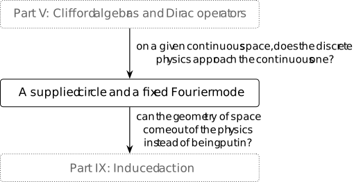
On a given continuous space, does the discrete physics approach the continuous one? The spatial Dirac calculation used lattice spacing one. Now supply a circle and place the graph on it. There are finitely many sites; the field values may still be real. For a field that changes over many vertices, the spacing is small relative to the scale of that change. Dividing an edge difference by the spacing then suggests a derivative. Continuous values concern the allowed field values, here real numbers; differentiability concerns the variation of a field on the supplied space and limits of difference quotients. Smoothness asks for derivatives of every order.
The circle calculation makes a limited comparison precise: each fixed Fourier mode of the discrete operator approaches its counterpart on the supplied circle. Approximation needs comparison maps and a limit; the chapter states these together with its pairings, positive precision and Gaussian moments. The circle is an input, so this result does not construct continuous space from the graph. The finite Dirac kernel in Proposition 16.3 depends on the parity of the periods; that separate calculation cautions against inferring a general continuum theory from one fixed-mode limit. Whether continuous-space physics can be recovered at large scales without supplying the space remains open here.
20.1. A supplied circle and a fixed Fourier mode [fdip-004G]AGENTDRAFTED
- October 31, 2026
20.1. A supplied circle and a fixed Fourier mode [fdip-004G]AGENTDRAFTED
- October 31, 2026
How does a finite operator approximate a differential operator when the circle and its length are already given? A periodic mesh, a normalized pairing and a positive mass give an explicit answer for each fixed Fourier mode. The same calculation controls one Gaussian second moment, using normalization and inverse-precision covariance. The spatial Dirac comparison provides related finite symbols; the scalar argument below does not require its Clifford module.
Definition 20.1.1. A circle mesh with normalized pairing [fdip-004H]AGENTDRAFTED
- October 31, 2026
Definition 20.1.1. A circle mesh with normalized pairing [fdip-004H]AGENTDRAFTED
- October 31, 2026
Supply the unit circle \(\mathbb R/\mathbb Z\), its coordinate \(x\) modulo one and length measure \(dx\). For an integer \(n\geq 3\), the circle mesh consists of the points \(j/n\), with \(j\in \mathbb Z/n\mathbb Z\), and spacing \(h_n=1/n\). Its real field space and reference pairing are \[E_n=\mathbb R^{\mathbb Z/n\mathbb Z},\qquad g_{0,n}(f,g)=\frac 1n\sum _{j=0}^{n-1}f_jg_j.\] On the complexification use \(\langle f,g\rangle _n=n^{-1}\sum _j\overline {f_j}g_j\); its restriction to real fields is \(g_{0,n}\).
Fix a mass squared \(\mu >0\), independent of \(n\). Define the cyclic shift, scaled nearest-neighbor Laplacian and precision by \[\begin {aligned} (T_nf)_j&=f_{j+1},\\ L_n&=n^2(2I-T_n-T_n^{-1}),\\ Q_n&=\mu I+L_n,\qquad q_n(f)=g_{0,n}(f,Q_nf). \end {aligned}\] Indices are taken modulo \(n\). These specialize the cyclic shift and difference energy, with the supplied scale \(n^2\). The scalar \(L_n\) is the nearest-neighbor operator compared with, and generally different from, the centered Dirac square in Proposition 16.3.
Periodic reindexing gives \(T_n^*=T_n^{-1}\) in the normalized pairing. Consequently \[\langle f,L_nf\rangle _n =n\sum _{j=0}^{n-1}|f_{j+1}-f_j|^2\geq 0.\] Thus \(Q_n\geq \mu I\) and \(Q_n\) is invertible, including on constant fields. This is the positive precision convention with the declared \(g_{0,n}\), rather than a change of the action form.
The step-function interpolation \(I_n\) assigns to \(f\) the function with value \(f_j\) whenever \(j/n\leq x<(j+1)/n\), using the representative \(0\leq x<1\). It maps real or complex fields into \(L^2(\mathbb R/\mathbb Z,dx)\), the square-integrable functions modulo almost-everywhere equality. Each interval has length \(1/n\), so \[\|I_nf\|_{L^2}^2=\frac 1n\sum _j|f_j|^2=\|f\|_n^2.\] Thus the comparison preserves the specified norm.
Example 20.1.2. Fourier modes and their Gaussian moments on a circle mesh [fdip-004I]AGENTDRAFTED
- October 31, 2026
Example 20.1.2. Fourier modes and their Gaussian moments on a circle mesh [fdip-004I]AGENTDRAFTED
- October 31, 2026
For the circle mesh, let \(k\in \mathbb Z\) and set \[e_k(x)=e^{2\pi ikx},\qquad e_{n,k}(j)=e^{2\pi ikj/n}.\] Every entry has modulus one, hence \(\|e_{n,k}\|_n=1\). Applying the shift and its inverse directly gives \[\begin {aligned} T_ne_{n,k}&=e^{2\pi ik/n}e_{n,k},\\ L_ne_{n,k}&=\lambda _{n,k}e_{n,k},\\ \lambda _{n,k} &=n^2(2-e^{2\pi ik/n}-e^{-2\pi ik/n})\\ &=4n^2\sin ^2(\pi k/n). \end {aligned}\] This derives the scaled version of the nearest-neighbor symbol. Frequencies differing by \(n\) give the same samples. For fixed \(k\ne 0\), the condition \(n>2|k|\) separates \(k\) from \(-k\) modulo \(n\).
For \(k=0\), \(e_{n,0}=\mathbf 1\) and \(\lambda _{n,0}=0\). For \(k=1\), a four-point mesh has \(\lambda _{4,1}=32\); an eight-point mesh has \(\lambda _{8,1}=64(2-\sqrt 2)\). The picture shows the supplied unit circle sampled at 4 equally spaced points. Its arrows indicate increasing \(j\); they do not specify a dynamics.
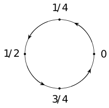
Now use real fields and the Gaussian law \[d\nu _n(f)=Z_n^{-1}e^{-q_n(f)/2}\,d\operatorname {vol}_{g_{0,n}}(f).\] In raw coordinates the volume and normalization are \[\begin {aligned} d\operatorname {vol}_{g_{0,n}}&=n^{-n/2}\,df_0\cdots df_{n-1},\\ Z_n&=(2\pi )^{n/2}(\det Q_n)^{-1/2}. \end {aligned}\] The volume factor follows because \(f\mapsto f/\sqrt n\) is an orthonormal chart; the partition function is Theorem 7.7. The covariance operator relative to \(g_{0,n}\) is \(Q_n^{-1}\) by Theorem 7.18. Since the exponent is \(f^TQ_nf/(2n)\), the raw coordinate covariance matrix is \(nQ_n^{-1}\).
Define the complex Fourier observable \(a_{n,k}=n^{-1}\sum _j e^{-2\pi ikj/n}f_j\). It has zero mean. Writing \(v=e_{n,k}\) and \(v^*\) for its conjugate transpose, the coordinate covariance gives \[\begin {aligned} \mathbb E_{\nu _n}|a_{n,k}|^2 &=n^{-2}v^*(nQ_n^{-1})v\\ &=\frac 1{\mu +\lambda _{n,k}}, \end {aligned}\] because \(v^*v=n\). All real and imaginary parts and their products are integrable polynomials by Proposition 7.11. In particular the real mean \(a_{n,0}\) has variance \(1/\mu \). At \(k=1\), the four-point and eight-point second moments are respectively \((\mu +32)^{-1}\) and \((\mu +64(2-\sqrt 2))^{-1}\).
For \(k\ne 0\) and \(n>2|k|\), put \[\begin {aligned} c_{n,k}&=\operatorname {Re}a_{n,k} =\frac 1n\sum _j\cos (2\pi kj/n)f_j,\\ s_{n,k}&=-\operatorname {Im}a_{n,k} =\frac 1n\sum _j\sin (2\pi kj/n)f_j. \end {aligned}\] The geometric sum \(\sum _j e^{4\pi ikj/n}=0\): its ratio is not one, its \(n\)-th power is one, and multiplying the sum by one minus the ratio gives zero. Taking real and imaginary parts, and using the double-angle identities, gives normalized squared norms \(1/2\) for both the cosine and sine vectors and their orthogonality. Both vectors have precision eigenvalue \(\mu +\lambda _{n,k}\), so Theorem 7.18 yields \[\operatorname {Var}(c_{n,k})=\operatorname {Var}(s_{n,k}) =\frac 1{2(\mu +\lambda _{n,k})}.\] The coefficients of the orthogonal projection \(A\cos (2\pi kj/n)+B\sin (2\pi kj/n)\) are \(A=2c_{n,k}\), \(B=2s_{n,k}\). Their variances are 4 times the displayed projection variances.
The character calculation and normalization above are direct
deductions from the cited finite operators and Gaussian results.
Mathlib's ZMod.dft uses the counting-measure forward sum;
\(a_{n,k}\) has the additional factor \(1/n\). This formal Fourier
transform is a supporting construction, not a formalization of the
mesh limit.
Proposition 20.1.3. A fixed Fourier mode and its massive inverse converge [fdip-004J]AGENTDRAFTED
- October 31, 2026
Proposition 20.1.3. A fixed Fourier mode and its massive inverse converge [fdip-004J]AGENTDRAFTED
- October 31, 2026
Use the circle meshes with fixed \(\mu >0\), and fix \(k\in \mathbb Z\) before letting \(n\to \infty \). For the Fourier modes and eigenvalues, \[\begin {aligned} \lambda _{n,k}&\longrightarrow 4\pi ^2k^2,\\ (\mu +\lambda _{n,k})^{-1} &\longrightarrow (\mu +4\pi ^2k^2)^{-1}. \end {aligned}\] Moreover, in \(L^2(\mathbb R/\mathbb Z,dx)\), \[I_nQ_n^{-1}e_{n,k} \longrightarrow (\mu +4\pi ^2k^2)^{-1}e_k.\] The vector on the right solves \(Au=e_k\) for \(A=-d^2/dx^2+\mu \) on smooth periodic functions. The selected Gaussian moment \(\mathbb E_{\nu _n}|a_{n,k}|^2\) converges to the same inverse eigenvalue.
Proof.
- October 31, 2026
Proof.
- October 31, 2026
For \(k=0\), the eigenvalue is identically zero and the sampled constant interpolates exactly to \(e_0=1\); all three assertions follow. For \(k\ne 0\), \[\lambda _{n,k} =4\pi ^2k^2\left (\frac {\sin (\pi k/n)}{\pi k/n}\right )^2.\] The sine quotient tends to one. Since \(\mu >0\), all denominators are at least \(\mu \), so continuity of inversion proves the scalar inverse limit.
For \(j/n\leq x<(j+1)/n\), the elementary inequality \(|e^{it}-e^{is}|\leq |t-s|\) gives \[|I_ne_{n,k}(x)-e_k(x)|\leq \frac {2\pi |k|}{n}.\] The inequality follows by integrating \(ie^{iu}\) between \(s\) and \(t\). The circle has measure one, hence the same bound holds for the \(L^2\) norm. Put \(b_n=(\mu +\lambda _{n,k})^{-1}\) and \(b=(\mu +4\pi ^2k^2)^{-1}\). Because \(|b_n|\leq 1/\mu \) and \(\|e_k\|_{L^2}=1\), \[\begin {aligned} \|b_nI_ne_{n,k}-be_k\|_{L^2} &\leq |b_n|\|I_ne_{n,k}-e_k\|_{L^2}+|b_n-b|\\ &\leq \frac {2\pi |k|}{\mu n}+|b_n-b|\longrightarrow 0. \end {aligned}\] The eigenvector equation identifies the left vector with \(I_nQ_n^{-1}e_{n,k}\). Differentiation gives \(Ae_k=(\mu +4\pi ^2k^2)e_k\). Finally the Gaussian second-moment formula in Example 20.1.2 is exactly \(b_n\).
This is an elementary limit deduction from the preceding finite
symbol, with an explicit interpolation map. Mathlib's
Real.tendsto_sin_div_nhdsNE_zero supplies the nonzero
sine-quotient limit used in the proof; the zero mode was handled
separately. The declaration does not supply the interpolation or
Gaussian comparison.
Remark 20.1.4. What the supplied-circle limit establishes [fdip-004K]AGENTDRAFTED
- October 31, 2026
Remark 20.1.4. What the supplied-circle limit establishes [fdip-004K]AGENTDRAFTED
- October 31, 2026
The fixed-mode limit compares finite operators and one Gaussian moment with a declared circle. Its length, measure, mesh spacing, factor \(n^2\) and positive mass are supplied. Without \(n^2\), each fixed-mode Laplacian eigenvalue tends to zero. This explains why a finite positive operator alone does not determine a continuum scale or geometry.
The quantifier on the frequency matters. For even \(n\) and \(k=n/2\), the discrete eigenvalue is \(4n^2\), whereas the continuum frequency has eigenvalue \(4\pi ^2k^2=\pi ^2n^2\). Their ratio stays \(4/\pi ^2\); the fixed-mode proof is therefore not a relative uniform estimate over all modes. It proves neither operator-norm resolvent convergence nor convergence of determinants or Gaussian measures. Removing the positive mass or adding interactions requires additional arguments.
For comparison, Weisz distinguishes the critical-point and phase-diagram control needed for low-energy lattice-QCD continuum limits from the renormalization questions for composite observables and high-energy scales [weisz2010renormalization, Section 1.1, printed p. 2]. The circle calculation is a much smaller prescribed approximation: it contains no interacting critical-point analysis. It establishes no emergent geometry, reflection positivity, Lorentzian reconstruction, Standard Model dynamics or gravitational dynamics. Those identifications remain among the open physical interfaces.
21. Realization and the information retained by observables [fdip-004L]AGENTDRAFTED
- November 1, 2026
21. Realization and the information retained by observables [fdip-004L]AGENTDRAFTED
- November 1, 2026
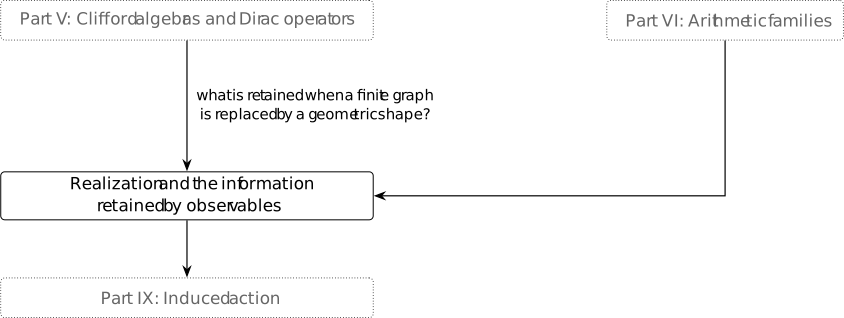
What is retained when a finite graph is replaced by a geometric shape? A graph records points and the links between them. One way to give it a shape is to assign an interval to each edge of its incidence presentation and join the intervals at their endpoints. Three edges in a cycle give a triangle's boundary; the graph alone does not choose its filling.
The retained Gaussian law gives a sharper test of the information preserved. Forget an edge weight while keeping its endpoint: two weights can then give the same interval but different variances at that endpoint. This is a small teaching variant of the weighted-cycle comparison, governed by the existing fiber-constancy criterion. An observable descends through the replacement exactly when it is constant on the data that the replacement identifies. Forgetting a weight can erase a retained observable even when the geometric construction is well-defined.
The enriched background comparison preserves observables only when the required data and the observables are transported together. The examples below identify what is forgotten and keep scalar factorization separate from categorical localization and gluing over covers. The shape is built by hand, just as the preceding approximation supplied its circle. Neither comparison supplies an emergent geometry or gluing theorem.
Definition 21.1. One-dimensional realization of finite incidence [fdip-004M]AGENTDRAFTED
- October 31, 2026
Definition 21.1. One-dimensional realization of finite incidence [fdip-004M]AGENTDRAFTED
- October 31, 2026
Let \(G=(V,E,s,h)\) be a finite incidence presentation. Its one-dimensional realization is the quotient space \[|G|=\bigl (V\sqcup (E\times [0,1])\bigr )/{\sim },\] where \(V,E\) are discrete, the intervals have their usual topology, and the equivalence relation is generated by \[(e,0)\sim s(e),\qquad (e,1)\sim h(e).\] Use the quotient topology. Thus each vertex is a point and each edge supplies an open interval attached at its endpoints, the standard one-dimensional CW construction of [hatcher2002algebraic, Section 1.A, p. 83]. Loops have both endpoints attached at one vertex; parallel edges remain separate intervals. Direction chooses the parametrization from \(0\) to \(1\), not a causal ordering.
Declare a morphism \(f:G\to G'\) to be a pair of maps \(f_V:V\to V'\) and \(f_E:E\to E'\) with \[f_Vs=s'f_E,\qquad f_Vh=h'f_E.\] It induces \[\begin {aligned} |f|:|G|&\longrightarrow |G'|,\\ [v]&\longmapsto [f_V(v)],\\ [e,t]&\longmapsto [f_E(e),t]. \end {aligned}\] These formulas respect the endpoint identifications. They are continuous before quotienting, so the quotient topology makes \(|f|\) continuous. Identity and composition follow from the formulas. This proves functoriality for these declared incidence maps; arbitrary edge contractions have not been included among them. The map construction is a direct deduction from the quoted quotient model.
Example 21.2. A triangle boundary and a filled triangle [fdip-004N]AGENTDRAFTED
- October 31, 2026
Example 21.2. A triangle boundary and a filled triangle [fdip-004N]AGENTDRAFTED
- October 31, 2026
Take the simple undirected triangle on vertices \(\{0,1,2\}\). Give its three edges any orientations, then forget them here; any parallel copies would also have to be merged before this simple undirected comparison. The one-dimensional realization retains the three edges without a face. In the nonempty-face convention of [maypishevar2025finitespaces, Definition 6.1.1, p. 61], its boundary complex and the filled complex have faces \[\begin {aligned} K_{\partial } &=\{\{0\},\{1\},\{2\},\{0,1\},\{1,2\},\{0,2\}\},\\ K_{\Delta }&=K_{\partial }\cup \{\{0,1,2\}\}. \end {aligned}\] The added face consists of three pairwise adjacent vertices: it is the filled clique triangle. This specifies these two complexes, without declaring a general clique-construction functor.
Choose three noncollinear points \(v_0,v_1,v_2\) in the plane. Realize each listed face by the convex hull of its vertices, as in [maypishevar2025finitespaces, Definitions 6.2.1 and 6.2.6, pp. 62-63]. Then \(|K_{\partial }|\) is the perimeter and \(|K_{\Delta }|\) is the closed triangular region. Traversing the three line segments identifies the perimeter with \([0,3]/(0\sim 3)\): the induced map is a continuous bijection from a compact space to a Hausdorff space, hence a homeomorphism. The map \(t\mapsto \exp (2\pi i t/3)\) gives the same identification with \(S^1\).
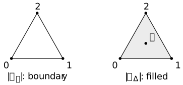
The filled triangle contracts to its barycenter \(b=(v_0+v_1+v_2)/3\) by \[H(x,t)=(1-t)x+tb,\qquad 0\leq t\leq 1.\] Convexity keeps \(H(x,t)\) in the triangle, and the formula is continuous, with \(H(x,0)=x\) and \(H(x,1)=b\). The two constructions have the same vertices and edges, but only the second supplies a two-dimensional face. Incidence alone therefore does not choose between keeping the perimeter and filling it. Each specified realization is nevertheless a well-defined construction.
These comparisons are elementary deductions from the cited
realization definitions. Mathlib's AbstractSimplicialComplex
uses nonempty faces and includes each vertex; its
Convex.contractibleSpace supplies contractibility of a
nonempty convex subset of a real topological vector space. These
support the conventions and the contraction step, not the complete
incidence-to-triangle comparison.
Definition 21.3. Forgetting a weight while retaining its endpoint [fdip-004O]AGENTDRAFTED
- October 31, 2026
Definition 21.3. Forgetting a weight while retaining its endpoint [fdip-004O]AGENTDRAFTED
- October 31, 2026
For each \(w>0\), let \(\mathcal B_w\) be the finite Gaussian background with vertices \(V=\{0,1\}\), one edge \(0\to 1\) of weight \(w\), counting pairing, mass \(m=1\), retained set \(R=\{0\}\) and eliminated set \(V\setminus R=\{1\}\). The field coordinates remain labelled. The weighted Laplacian and massive precision are \[\begin {aligned} L_w&=w\begin {pmatrix}1&-1\\-1&1\end {pmatrix},\\ Q_w&=I+L_w=\begin {pmatrix}1+w&-w\\-w&1+w\end {pmatrix}. \end {aligned}\] Indeed the incidence row is \((-1,1)\). The vectors \((1,1)\) and \((1,-1)\) have precision eigenvalues \(1\) and \(1+2w\), so \(Q_w>0\). The normalized Gaussian law is therefore well-defined on counting-coordinate volume \(df_0\,df_1\), with \[\begin {aligned} d\mu _w(f)&=Z_w^{-1}\exp (-f^TQ_wf/2)\,df_0\,df_1,\\ Z_w&=\frac {2\pi }{\sqrt {1+2w}}. \end {aligned}\] The normalizer is the two-dimensional specialization of positive Gaussian normalization.
Let \(X=\{\mathcal B_w:w>0\}\) and let \(Y=\{U\}\) be the singleton whose element is the unweighted labelled directed edge \(0\to 1\) with distinguished endpoint \(0\). Define \[\begin {aligned} c:X&\longrightarrow Y,&c(\mathcal B_w)&=U,\\ r:X&\longrightarrow \mathbb R,&r(\mathcal B_w)&=\int f_0^2\,d\mu _w(f). \end {aligned}\] Thus \(c\) forgets the varying weight while retaining the labels, orientation and selected endpoint; the mass and reference pairing are fixed throughout the family. The observable is integrable by Gaussian polynomial integrability. The coordinate has zero mean, so \(r\) is the variance at the retained endpoint. Composing \(c\) with the interval realization gives the same labelled interval with that endpoint for every \(w\).
Example 21.4. The retained variance detects the forgotten weight [fdip-004P]AGENTDRAFTED
- October 31, 2026
Example 21.4. The retained variance detects the forgotten weight [fdip-004P]AGENTDRAFTED
- October 31, 2026
For the two-vertex family, eliminate the coordinate at vertex \(1\). The positive Schur formula and retained covariance give \[\begin {aligned} S_w&=(1+w)-\frac {w^2}{1+w} =\frac {1+2w}{1+w}>0,\\ r(\mathcal B_w)&=S_w^{-1}=\frac {1+w}{1+2w}. \end {aligned}\] In particular, \[r(\mathcal B_1)=\frac 23\ne \frac 35=r(\mathcal B_2), \qquad c(\mathcal B_1)=c(\mathcal B_2)=U.\] The fiber-constancy criterion excludes a function \(F:c(X)\to \mathbb R\) satisfying \(r=F\circ c\), even on a restricted family containing these two backgrounds. Consequently the unweighted interval with its retained endpoint also cannot recover this variance on that family. This is an obstruction for the specified forgetting and observable, not for every geometric realization.
This two-coordinate calculation is a teaching variant of the weighted-cycle comparison, which already gives unequal retained correlations \(2/15\) and \(16/105\) at fixed mass and fixed retained pair. The same principle is visible with one retained coordinate: incidence and the selected endpoint do not retain the weighted precision. By contrast, weight-preserving relabelings, with the retained projection and observable transported together, preserve expectations by Gaussian transport. Enlarging their comparison to forget weights need not preserve them.
Remark 21.5. Scalar factorization, localization and gluing [fdip-004Q]AGENTDRAFTED
- October 31, 2026
Remark 21.5. Scalar factorization, localization and gluing [fdip-004Q]AGENTDRAFTED
- October 31, 2026
The retained-variance example tests scalar factorization: for specified functions \(c:X\to Y\) and \(r:X\to \mathbb R\), it asks whether \(r=F\circ c\) for a function on \(c(X)\). The fiber criterion answers exactly this question, without supplying continuity or any categorical structure.
Functorial factorization instead starts with categories and
functors \(U:\mathcal B\to \mathcal D\) and
\(O:\mathcal B\to \mathcal A\), and asks for
\(\overline O:\mathcal D\to \mathcal A\) and a
natural isomorphism
\(O\cong \overline O\circ U\). A localization at a declared
class \(W\) of arrows has an additional universal property: it
inverts those arrows and is universal among functors that do so
[stacks2017stacks, Section 4.27], Tag 04VB.
A generic forgetful functor is not thereby a localization.
Mathlib's CategoryTheory.Localization.lift requires
both a localization functor and a functor that inverts \(W\);
these hypotheses are absent from the scalar example.
Local-to-global descent requires a site with covers, restriction maps and compatible data on overlaps, together with an effective gluing statement. For category-valued data, a stack also requires a fibred category and sheaves of morphisms [stacks2017stacks, Definition 8.4.1], Tag 0268. The enriched background groupoid and the scalar variance calculation supply none of this cover-and-gluing structure. The groupoid is a category of finite backgrounds, not necessarily a finite category. No local-to-global descent theorem follows.
22. Selected backgrounds and invariants [fdip-0059]AGENTDRAFTED
- November 1, 2026
22. Selected backgrounds and invariants [fdip-0059]AGENTDRAFTED
- November 1, 2026
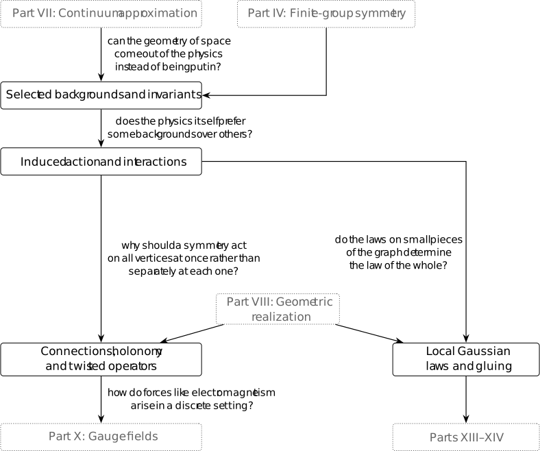
Can geometry be induced instead of supplied? Edge weights set the stiffness of field differences and may encode geometric information; they are not universally distances. Comparing choices through an induced action first requires keeping the graph data distinct from the choice of which field to retain. A retained field need not consist of named vertex coordinates. It may be a symmetry sector, or another specified subspace of the vertex fields. An orthogonal projector records this choice relative to the counting metric. Integrating out its orthogonal complement produces a Gaussian law on the chosen subspace.
The graph and its selector remain separate data. A graph relabeling must transport both, while an arbitrary orthogonal comparison of precisions can forget incidence. The examples below compare three selectors on one four-cycle and two rank-4 selectors on a quaternion Cayley graph. Their retained spectra separate choices that the unselected graph cannot distinguish. The restriction criterion then identifies exactly when eliminating the complement changes the compressed precision; a stable prism line shows why group symmetry alone is insufficient. In this chapter \(\Gamma \) denotes a symmetry group and \(G=Q^{-1}\) denotes the Green operator.
Definition 22.1. A selected Gaussian background [fdip-005A]AGENTDRAFTED
- November 1, 2026
Definition 22.1. A selected Gaussian background [fdip-005A]AGENTDRAFTED
- November 1, 2026
A selected Gaussian background is a tuple \[b=(\Pi ,w,m,P),\qquad \Pi =(V,E,s,h),\] where \(\Pi \) is a finite incidence presentation, \(w:E\to \mathbb R_{>0}\), \(m>0\), and \(P\) is an orthogonal projector on the counting inner-product space \(H=\mathbb R^V\), with \[P^2=P=P^*,\qquad 0<\operatorname {rank}P<|V|.\] The selected space is \(X=\operatorname {im}P\), its orthogonal complement is \(Y=\ker P\), and the observed random vector is \(P\phi \in X\). Incidence, the Green operator and the full law are \[\begin {aligned} (d\phi )(e)&=\phi (h(e))-\phi (s(e)),\\ Q&=d^*Wd+m^2I>0,\qquad G=Q^{-1},\\ \phi &\sim \mu _Q. \end {aligned}\] Here \(W=\operatorname {diag}(w)\) and \(\mu _Q\) uses the induced Euclidean volume. These are derived from the tuple, not additional choices.
Three constructions supply such projectors, provided their ranks are nonzero and proper.
- A retained subset \(R\subsetneq V\) gives \(P_R\phi =\sum _{v\in R}\phi (v)\delta _v\). Identifying \(\operatorname {im}P_R\) with \(\mathbb R^R\) recovers the coordinate background.
- A finite signed graph symmetry \(\rho :\Gamma \to O(H)\) extends to \(\mathbb R[\Gamma ]\). For \(e^2=e=e^*\), where \([g]^*=[g^{-1}]\), \(P=\rho (e)\) is orthogonal because \(\rho (e)^*=\rho (e^*)\). The precision commutes with every \(\rho (g)\), hence with this \(P\).
- For a \(\Gamma \)-stable subspace \(X\subset H\), its orthogonal projector commutes with \(\rho (\Gamma )\): orthogonality makes \(X^\perp \) stable too. It need not commute with \(Q\). Within a repeated real isotypic block, the chosen multiplicity subspace may fail to be invariant under the positive multiplicity matrix. These are different constructions: a subrepresentation projector commutes with \(\rho (\Gamma )\) but need not commute with \(Q\); a group-algebra projector commutes with \(Q\) but need not commute with \(\rho (\Gamma )\). Centrality of \(e\) is sufficient for the latter commutation, and hence for a stable image.
Every subspace has a unique orthogonal projector for the specified metric. This makes the selector equivalent to choosing \(X\), without choosing an additional complementary subspace. An oblique idempotent \(T^2=T\) also gives a Gaussian observation \(T\phi \), and orthogonal conjugation does transport it naturally: \(T\mapsto OTO^{-1}\). But it also records a possibly nonorthogonal kernel, so the image alone no longer determines the observation or its covariance \(TGT^*\). General linear observations are outside this definition. No physical rule selecting \(P\) from an environment is assumed.
Theorem 22.2. The law on a selected subspace [fdip-005B]AGENTDRAFTED
- November 1, 2026
Theorem 22.2. The law on a selected subspace [fdip-005B]AGENTDRAFTED
- November 1, 2026
For a selected background, view \(P\) as a map \(H\to X=\operatorname {im}P\) and let \(r=\dim X\). The law \(\nu _b=P_*\mu _Q\) is the centered Gaussian on \(X\) with intrinsic covariance and precision \[C_P=(PGP)|_X>0,\qquad S_P=C_P^{-1}:X\to X.\] Relative to the induced Euclidean volume \(\lambda _X\), its density is \[\frac {d\nu _b}{d\lambda _X}(x) =\frac {\sqrt {\det _X S_P}}{(2\pi )^{r/2}} e^{-\langle x,S_Px\rangle /2}.\] If \(B:\mathbb R^r\to H\) is an isometric inclusion with image \(X\), then \(BB^*=P\); its chosen coordinate matrices are \[B^*C_PB=B^*GB,\qquad [S_P]_B=(B^*GB)^{-1}.\] For another such basis \(B'=BU\), \(U\in O(r)\), the latter changes to \(U^*[S_P]_BU\). The intrinsic operator \(S_P\) is independent of this choice.
Proof.
- November 1, 2026
Proof.
- November 1, 2026
For nonzero \(x\in X\), \(\langle x,C_Px\rangle =\langle x,Gx\rangle >0\). Set \(C=B^*GB\), so \(C>0\). The positive square roots of \(Q\) and \(C\) exist by the real spectral theorem. The density change of variables \(z=Q^{1/2}\phi \) gives the standard Gaussian density \((2\pi )^{-|V|/2}e^{-|z|^2/2}\): its Jacobian and the normalizer cancel. Put \[T=C^{-1/2}B^*Q^{-1/2}.\] Then \(TT^*=C^{-1/2}(B^*GB)C^{-1/2}=I_r\), so its rows extend to an orthonormal basis of \(H\). The resulting square orthogonal matrix carries \(z\) to a standard Gaussian, since its Jacobian has absolute value one and it preserves the squared norm. Its first \(r\) coordinates are \(Tz\); integration over the other coordinates gives the standard \(r\)-dimensional density. Hence \[B^*\phi =C^{1/2}Tz\] has density \((2\pi )^{-r/2}(\det C)^{-1/2} e^{-y^TC^{-1}y/2}\) by an invertible change of variables. The isometry \(B\) carries Euclidean volume to \(\lambda _X\) and \(B(B^*\phi )=P\phi \). This proves the law and its density, rather than inferring a law from its covariance alone.
For \(x,x'\in X\), the covariance of the corresponding linear observations is \(\langle x,Gx'\rangle =\langle x,C_Px'\rangle \) by the inverse-precision formula. The inverse identity and \(B'=BU\) give the coordinate statements.
In the orthogonal split \(H=X\oplus Y\), write \[Q=\begin {pmatrix}A&K\\K^*&D\end {pmatrix},\qquad D>0.\] Then \[S_P=A-KD^{-1}K^*.\] Indeed, solving \(Q(x,y)=(u,0)\) gives \(y=-D^{-1}K^*x\) and \((A-KD^{-1}K^*)x=u\). Positivity follows by evaluating the quadratic form on \((x,-D^{-1}K^*x)\). Thus the \(X,X\) block of \(Q^{-1}\) is the inverse of this Schur complement, and it is exactly \(C_P\). For \(P=P_R\), this recovers the coordinate marginal. If \(PQ=QP\), then \(K=0\) and \(S_P=Q|_X\); symmetry of a subspace alone does not justify that equality.
[rasmussen2006gaussian, Appendix A.2, p. 200] gives formulas (A.4)-(A.6) for Gaussian densities and marginals.
[friedli2017statistical, Definition 8.3, p. 384] characterizes Gaussian vectors by linear observations.
[friedli2017statistical, Theorem 8.4, p. 385] gives their nonsingular density. The row-isometry argument above supplies the linear-image step, including its Euclidean-volume identification.
A partial formal correspondence is supplied by TauCeti's
TauCeti.Probability.map_affine_multivariateGaussian.
It allows finite real coordinate spaces, a positive semidefinite
covariance and an arbitrary rectangular linear map. Set its mean
and shift to zero, its covariance to \(G=Q^{-1}>0\), and its matrix
to \(B^*\). After the precision-density identification,
the result gives the coordinate image law with covariance \(B^*GB\).
It does not require full row rank. Positivity of this compressed
covariance, its inverse precision, the isometric identification
with \(X\), and the graph data are the additional arguments above.
Definition 22.3. Arrows of selected backgrounds [fdip-005C]AGENTDRAFTED
- November 1, 2026
Definition 22.3. Arrows of selected backgrounds [fdip-005C]AGENTDRAFTED
- November 1, 2026
The groupoid \(\mathsf {Bg}\) has selected backgrounds as objects. An arrow \(b\to b'\) is a pair of bijections \(p:V\to V'\), \(q:E\to E'\) satisfying \[\begin {aligned} s'q&=ps,&h'q&=ph,\\ w'q&=w,&m'&=m,\\ P'&=UPU^{-1},&&(U\phi )(p(v))=\phi (v). \end {aligned}\] Here \(U:H\to H'\) is the vertex counting isometry, distinct from the selector \(P\). For coordinate selectors the last equation is equivalent to \(pR=R'\), so these are precisely the exact relabelings.
The larger groupoid \(\mathsf {Bg}^{\pm }\) allows signed endpoint arrows: an additional sign \(\varepsilon (e)\in \{+,-\}\) specifies whether \(q(e)\) has endpoints \((ps(e),ph(e))\) or \((ph(e),ps(e))\). Weights, mass and the selector obey the same equations. The signed edge map is \((Ja)(q(e))=\varepsilon (e)a(e)\), where the sign acts as \(\pm 1\). Then \(d'U=Jd\) and \(W'J=JW\). Consequently \[Q'=UQU^{-1},\qquad G'=UGU^{-1}.\] The endpoint condition is retained even for loops of zero incidence. Signs are part of an arrow, not merely an equation between Laplacians.
Compose vertex and edge bijections, and for signed arrows use \[\varepsilon _{21}(e)=\varepsilon _2(q_1(e))\varepsilon _1(e).\] The identity has identity bijections and positive signs; the inverse has inverse bijections and sign \(\varepsilon (e)\) at \(q(e)\). The endpoint-arrow proof checks all graph equations. Selector transport also composes because \(P''=U_2U_1P(U_2U_1)^{-1}\). It inverts by conjugating back. These operations therefore give groupoids on the stated tuples.
Restrict \(U\) to the isometry \(U_X:X\to X'\) of selected spaces. Then the selected laws satisfy \[\begin {aligned} C_{P'}&=U_XC_PU_X^{-1},\\ S_{P'}&=U_XS_PU_X^{-1},\\ (U_X)_*\nu _b&=\nu _{b'}. \end {aligned}\] For the first identity insert \(P'=UPU^{-1}\) and \(G'=UGU^{-1}\); inversion gives the second. The full-law transport gives \(U_*\mu _Q=\mu _{Q'}\), while \(P'U=U_XP\). Composition of Borel pushforwards proves the third. In particular, for an integrable retained observable \(F'\) on \(X'\), \[\int _{X'}F'\,d\nu _{b'}=\int _X F'\circ U_X\,d\nu _b.\] The equality for \(|F'|\), allowing infinity, first establishes the matching integrability condition.
These arrows carry incidence, not only the precision and projector. Replacing one edge of weight \(w\) by two parallel edges with the same endpoints and positive weights summing to \(w\) leaves \(Q\) unchanged, but changes \(|E|\); it admits no arrow in either groupoid. Reversing the orientation of a specified edge gives an identity-on-vertices signed arrow with negative sign on that edge. That particular correspondence is not directed. Another directed isomorphism may exist if the graph has additional symmetries.
Definition 22.4. The orthogonal comparison of selected precisions [fdip-005D]AGENTDRAFTED
- November 1, 2026
Definition 22.4. The orthogonal comparison of selected precisions [fdip-005D]AGENTDRAFTED
- November 1, 2026
The orthogonal comparison of selected precisions is \[(Q,P)\sim _O(Q',P')\] when there is an orthogonal isomorphism \(O:H\to H'\) with \(Q'=OQO^{-1}\) and \(P'=OPO^{-1}\). It is an equivalence relation by identity, inverse and composition. Every background arrow supplies such a comparison. The same proof transports the selected law by \(O|_X\), but an arbitrary \(O\) need not transport vertex or edge labels. This relation differs both from the scaled Laplacian relation, which forgets mass and selector, and from general linear transport, which may change the specified metric.
The cospectral graph example proves that this comparison can identify selected backgrounds with nonisomorphic graphs. Their graph and orthogonal stabilizers also carry different information.
Example 22.5. Cospectral graphs with the same selector [fdip-005H]AGENTDRAFTED
- November 1, 2026
Example 22.5. Cospectral graphs with the same selector [fdip-005H]AGENTDRAFTED
- November 1, 2026
There are selected backgrounds related by the orthogonal comparison with no signed graph arrow. On vertices \(\{0,1,2,3,4,5\}\), take simple graphs with unit weights and the following unordered edges: \[\begin {aligned} E_A&=\{02,03,04,05,14,15,23\},\\ E_B&=\{02,04,05,12,14,15,23\}. \end {aligned}\] Orient each edge from its lower to its higher endpoint, choose \(m=1\), and in both cases choose \(P=\mathbf 1\mathbf 1^T/6\), the projector onto the constant line. Both graphs are connected. Their degree multisets are \((4,2,2,2,2,2)\) and \((3,3,3,2,2,1)\), so even their unoriented incidence presentations are not isomorphic.
Proof.
- November 1, 2026
Proof.
- November 1, 2026
For graph \(A\), the differences on the twin pairs \(\{2,3\}\) and \(\{4,5\}\) have Laplacian eigenvalues \(3\) and \(2\). On fields constant on the cells \(\{0\}\), \(\{1\}\), \(\{2,3\}\), \(\{4,5\}\), in that order, the remaining matrix is \[M_A=\begin {pmatrix} 4&0&-2&-2\\0&2&0&-2\\-1&0&1&0\\-1&-1&0&2 \end {pmatrix}.\] For graph \(B\), use twin differences on \(\{0,1\}\) and \(\{4,5\}\), again of eigenvalues \(3\) and \(2\). On cells \(\{0,1\}\), \(\{2\}\), \(\{3\}\), \(\{4,5\}\), in that order, the matrix is \[M_B=\begin {pmatrix} 3&-1&0&-2\\-2&3&-1&0\\0&-1&1&0\\-2&0&0&2 \end {pmatrix}.\] These are cell-value coordinates, so the displayed quotient matrices need not be symmetric. In each case expansion gives \[\det (tI-M_A)=\det (tI-M_B)=t(t-3)(t^2-6t+4).\] Together with the two difference eigenvectors, this proves the common Laplacian spectrum \(0,2,3,3,3-\sqrt 5,3+\sqrt 5\). Choose orthonormal eigenbases with the same normalized constant vector \(\mathbf 1 / \sqrt 6\) first, and map one basis to the other. The resulting \(O\) conjugates \(L_A\) to \(L_B\), hence also \(Q_A=L_A+I\) to \(Q_B=L_B+I\). It fixes the constant line and therefore transports \(P\) as well. This proves the selected comparison. The degree multisets exclude every signed graph arrow.
Proposition 22.6. Graph and orthogonal stabilizers [fdip-005I]AGENTDRAFTED
- November 1, 2026
Proposition 22.6. Graph and orthogonal stabilizers [fdip-005I]AGENTDRAFTED
- November 1, 2026
The stabilizers also distinguish the two notions. For the alternating four-cycle family, with weights \((a,b,a,b)\), \(m>0\), and \(R=\{0,2\}\), the stabilizer of \((Q,P_R)\) in \(O(4)\) is \((C_2)^2\) if \(a\ne b\), and \((C_2)^3\) if \(a=b\). The signed graph stabilizers are respectively \(C_2\) and \(C_2\times C_2\). By contrast, the orthogonal stabilizer of \(Q\) alone is continuous when \(a=b\); it contains \(O(2)\) on the repeated eigenspace.
Proof.
- November 1, 2026
Proof.
- November 1, 2026
Use the orthonormal eigenvectors \[\begin {aligned} u_0&=(1,1,1,1)/2,&u_3&=(1,-1,1,-1)/2,\\ u_1&=(1,1,-1,-1)/2,&u_2&=(1,-1,-1,1)/2. \end {aligned}\] Their eigenvalues are \(m^2,m^2+2a+2b,m^2+2b,m^2+2a\), respectively. In the ordered pairs \((u_0,u_3)\) and \((u_1,u_2)\), \(P_R\) has the same block \(\frac 12\begin {pmatrix}1&1\\1&1\end {pmatrix}\). If \(a\ne b\), all 4 eigenvalues are distinct, so an orthogonal commuter of \(Q\) chooses one sign on each eigenline. Commuting with \(P_R\) makes the signs equal within each pair, leaving two independent signs. If \(a=b\), the first pair still shares one sign. On \(\operatorname {span}(u_1,u_2)\), an orthogonal commuter must preserve the two lines spanned by \(u_1+u_2\) and \(u_1-u_2\), leaving two further signs. This proves the orthogonal counts.
For a signed graph symmetry \(r^ks^\epsilon \) with \(r(i)=i+1\), \(s(i)=-i\), the opposite set is preserved iff \(k\) is even. When \(a\ne b\), weight preservation additionally requires \(k+\epsilon \) even. Thus only \(1,r^2\) remain; when \(a=b\), \(1,r^2,s,r^2s\) remain. These are all possibilities because the underlying simple-cycle automorphism group is \(D_4\), as in Example 17.1.
Definition 22.7. The base and its retained-law fibers [fdip-005E]AGENTDRAFTED
- November 1, 2026
Definition 22.7. The base and its retained-law fibers [fdip-005E]AGENTDRAFTED
- November 1, 2026
Fix an incidence presentation \(\Pi =(V,E,s,h)\), with \(|V|\ge 2\). Its parameter set and selector set are \[\begin {aligned} \operatorname {Par}_{\Pi }&=\mathbb R_{>0}^E\times \mathbb R_{>0},\\ \operatorname {Sel}_V&=\{P:P^2=P=P^*,\ 0<\operatorname {rank}P<|V|\},\\ \mathcal B_\Pi &=\operatorname {Par}_\Pi \times \operatorname {Sel}_V. \end {aligned}\] The counting metric is fixed. Each rank component of \(\operatorname {Sel}_V\) identifies with the real Grassmannian \(\operatorname {Gr}_r(H)\), the set of \(r\)-dimensional subspaces of \(H\), by \(P\mapsto \operatorname {im}P\); the unique orthogonal projector gives the inverse identification. No topology or smooth structure is needed for the following groupoid description.
Only the directed automorphism group \(\operatorname {Aut}(\Pi )\) acts on this fixed-presentation set. For \(g=(p,q)\), let \(U_g\delta _v=\delta _{p(v)}\) and put \[g(w,m,P)=(w\circ q^{-1},m,U_gPU_g^{-1}).\] Its action groupoid \(\operatorname {Aut}(\Pi )\ltimes \mathcal B_\Pi \) is the full subgroupoid of \(\mathsf {Bg}\) on backgrounds whose presentation is exactly \(\Pi \): in both cases arrows are precisely the same graph automorphisms satisfying the parameter equations. Replacing directed automorphisms by signed endpoint automorphisms gives the corresponding full subgroupoid of \(\mathsf {Bg}^{\pm }\).
To allow arrows between presentations, take \(\mathcal B=\coprod _\Pi \mathcal B_\Pi \), over a fixed set of finite labelled presentations, with \(\mathsf {Bg}\) as its groupoid of arrows. For example one may use finite subsets of a fixed countable universe as carriers; every finite presentation has an isomorphic labelled representative. There is no single action of \(\operatorname {Aut}(\Pi )\) on all presentations.
The selected-structure map is \[\sigma :\mathcal B\longrightarrow \operatorname {Ob}(\mathcal Q),\qquad \sigma (b)=(X,S_P),\quad X=\operatorname {im}P,\] where \(\mathcal Q\) is the groupoid of positive-dimensional real Euclidean spaces with positive self-adjoint precisions and isometric precision-intertwining arrows. More precisely, the displayed object map extends to a functor \(\mathsf {Bg}\to \mathcal Q\), or \(\mathsf {Bg}^{\pm }\to \mathcal Q\), by sending an arrow to \(U|_X\). The transport identities and ordinary restriction of composites prove functoriality. The symbol \(\sigma \) denotes this assignment, whereas \(P:H\to H\) is the field-space projector.
The retained-law fiber over \(b\) is the probability space \[\mathcal F_b=(X,\mathcal B(X),\nu _b),\qquad \nu _b=N_X(0,S_P^{-1}).\] Here \(\mathcal B(X)\) is the Borel sigma-algebra. Arrows transport these fibers by measure-preserving isometries and transport observables by pullback. Thus a fiber is a specified law on a specified space, rather than a bare covariance matrix. If an interaction is additionally supplied, its induced retained vertices require that further data; they are not part of the present Gaussian tuple.
Forgetting \(P\) gives the unselected weighted incidence data \((\Pi ,w,m)\) and their full law \(\mu _Q\). It does not by itself give a coordinate background, which also requires a retained subset \(R\). Choosing \(P=P_R\) recovers that background and its Schur marginal. Equivalence here means isomorphism in the chosen graph groupoid; the orthogonal comparison is coarser. For a different operation, the supplied cycle scaling of the circle comparison is a limit of models, not a graph arrow.
Example 22.8. Three selectors on the same four-cycle [fdip-005F]AGENTDRAFTED
- November 1, 2026
Example 22.8. Three selectors on the same four-cycle [fdip-005F]AGENTDRAFTED
- November 1, 2026
Take the unit four-cycle, \(m=1\), and vertex order \((0,1,2,3)\). Its full precision and covariance are \[\begin {aligned} Q&=\begin {pmatrix} 3&-1&0&-1\\-1&3&-1&0\\0&-1&3&-1\\-1&0&-1&3 \end {pmatrix},\\ G&=\frac 1{15}\begin {pmatrix} 7&3&2&3\\3&7&3&2\\2&3&7&3\\3&2&3&7 \end {pmatrix}. \end {aligned}\] Multiplication gives \(QG=I\); the full spectrum is \(1,3,3,5\). The graph and full law stay fixed in all three selections below.
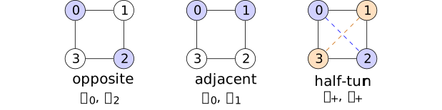
In the first two panels, filled vertices are retained coordinates. In the third, the paired colors and dashed diagonals indicate the normalized sums \(x_+=(\phi _0+\phi _2)/\sqrt 2\) and \(y_+=(\phi _1+\phi _3)/\sqrt 2\); the diagonals are pairing guides, not added graph edges. All three observations have rank two.
For \(R=\{0,2\}\), use the orthonormal retained basis \((\delta _0,\delta _2)\). Compressing \(G\) and inverting gives \[\begin {aligned} C_{\mathrm {opp}}&=\frac 1{15}\begin {pmatrix}7&2\\2&7\end {pmatrix},\\ S_{\mathrm {opp}}&=\frac 13\begin {pmatrix}7&-2\\-2&7\end {pmatrix}. \end {aligned}\] The sum and difference vectors have precision eigenvalues \(5/3,3\); their product is \(\det S_{\mathrm {opp}}=5\). This is the opposite-vertex marginal.
For \(R=\{0,1\}\), use \((\delta _0,\delta _1)\). The same operation yields \[\begin {aligned} C_{\mathrm {adj}}&=\frac 1{15}\begin {pmatrix}7&3\\3&7\end {pmatrix},\\ S_{\mathrm {adj}}&=\frac 18\begin {pmatrix}21&-9\\-9&21\end {pmatrix}. \end {aligned}\] Its sum and difference eigenvalues are \(3/2,15/4\), with \(\det S_{\mathrm {adj}}=45/8\). This recovers the fixed-label counterexample as a change of selector.
Finally let \(H_2\delta _i=\delta _{i+2}\) be the half-turn and \(P_+=(I+H_2)/2\). In the orthonormal basis \[v_0=(\delta _0+\delta _2)/\sqrt 2,\qquad v_1=(\delta _1+\delta _3)/\sqrt 2\] of its image, the positive sector has \[\begin {aligned} C_+&=\frac 15\begin {pmatrix}3&2\\2&3\end {pmatrix},\\ S_+&=\begin {pmatrix}3&-2\\-2&3\end {pmatrix}. \end {aligned}\] Indeed \(Qv_0=3v_0-2v_1\) and \(Qv_1=-2v_0+3v_1\), so this space is \(Q\)-invariant and the retained precision is the restriction. Its eigenvalues are \(1,5\), with determinant \(5\). The coordinates are normalized sums \((\phi _0+\phi _2)/\sqrt 2\), \((\phi _1+\phi _3)/\sqrt 2\), not the values of two retained vertices.
All three laws follow from the selected-law theorem with the displayed basis choices. Equal rank, or even the shared determinant \(5\) of the first and third examples, does not force equal retained spectra.
Example 22.9. Quaternion and coordinate selectors [fdip-005G]AGENTDRAFTED
- November 1, 2026
Example 22.9. Quaternion and coordinate selectors [fdip-005G]AGENTDRAFTED
- November 1, 2026
Let \(\Gamma =Q_8=\{\pm 1,\pm i,\pm j,\pm k\}\) and take the simple undirected Cayley graph with edges \(\{g,gs\}\), \(s\in \{\pm i,\pm j\}\), counted once each. Give each edge weight one, choose any orientation, and set \(m=1\). The two parts \[A=\{\pm 1,\pm k\},\qquad B=\{\pm i,\pm j\}\] give \(K_{4,4}\): every vertex in one part has the 4 distinct vertices of the other as its neighbors. In part order, \[L=\begin {pmatrix}4I_4&-J_4\\-J_4&4I_4\end {pmatrix}, \qquad Q=L+I_8,\] where \(J_4\) is the all-ones matrix. The two constant-on-part vectors give Laplacian eigenvalues \(0,8\); the two partwise zero-sum spaces give eigenvalue \(4\), of total multiplicity 6.
Left multiplication gives a signed graph action \(\rho \) on \(\mathbb R^{Q_8}\), independent of the arbitrary edge orientations. For the central involution \(z=-1\), put \[e_-=(1-[z])/2\in \mathbb R[Q_8],\qquad P_-=\rho (e_-)=(I-\rho (z))/2.\] Since \(z^2=1\) and \(z^{-1}=z\), this is a self-adjoint idempotent. Its image is the four-dimensional space of fields \(f(-g)=-f(g)\). The group-algebra decomposition \(\mathbb R[Q_8]\cong \mathbb R^4\times \mathbb H\) in Proposition [fgap-001B] sends \(e_-\) to \((0,1)\): each real character takes \(z\) to \(1\), while the quaternionic realization takes it to \(-1\). Thus this selector retains precisely the quaternion factor in the regular module, without assigning it a physical interpretation.
Proof.
- November 1, 2026
Proof.
- November 1, 2026
An odd field has zero sum on each of \(A,B\), since each part is a union of pairs \(\{g,-g\}\). Therefore \(J_4\) kills its restriction to either part, and the displayed Laplacian gives \(Lf=4f\). An orthonormal basis is \((\delta _g-\delta _{-g})/\sqrt 2\) for \(g=1,i,j,k\). Hence the selected precision is \[S_-=5I_4,\qquad C_-=I_4/5.\] Equivalently, the two neighbor contributions indexed by \(s,-s\) cancel on an odd field. The positive mass supplies the shift from \(4\) to \(5\).
Compare the coordinate selector on the subgroup \(R=\langle i\rangle =\{1,-1,i,-i\}\), which retains two vertices from each part. In the full graph, decompose fields into the two constant-on-part lines and the two partwise zero-sum spaces. On the normalized part constants, the precision and covariance are \[\begin {pmatrix}5&-4\\-4&5\end {pmatrix},\qquad \frac 19\begin {pmatrix}5&4\\4&5\end {pmatrix};\] on the zero-sum spaces the covariance is \(1/5\). It follows that full covariance entries are \(13/45\) on the diagonal, \(4/45\) between distinct vertices in the same part, and \(1/9\) between parts. For example the first entry is \((1-1/4)/5+(5/9)/4=13/45\).
In retained order \((1,-1,i,-i)\), compression therefore gives \[C_R=\frac 1{45}\begin {pmatrix} 13&4&5&5\\4&13&5&5\\5&5&13&4\\5&5&4&13 \end {pmatrix}.\] The two within-part difference vectors have covariance eigenvalue \((13-4)/45=1/5\). On normalized retained part constants the covariance block is \(\frac 1{45}\begin {pmatrix}17&10\\10&17\end {pmatrix}\), with eigenvalues \(3/5,7/45\). Inversion gives the retained precision spectrum \[\operatorname {spec}(S_R)=\{5/3,5,5,45/7\}.\] It differs from \(\{5,5,5,5\}\) for the quaternion selector despite equal rank and the same full background precision.
The chosen \(Q_8\) action is auxiliary data used to construct \(P_-\); it is not another slot of the selected tuple. Indeed the underlying graph has \(2(4!)^2=1152\) automorphisms: its connected bipartition is unique up to exchange, and every permutation within either part, as well as their exchange, preserves all edges. The selected-background groupoid remembers the graph and the resulting projector, not a named subgroup of this automorphism group. Remembering the action would require an enhanced tuple and arrows intertwining that action.
Proposition 22.10. Invariants of a selected background [fdip-005J]AGENTDRAFTED
- November 1, 2026
Proposition 22.10. Invariants of a selected background [fdip-005J]AGENTDRAFTED
- November 1, 2026
For a selected background, put \(X=\operatorname {im}P\). The following are invariants of its orthogonal comparison class:
- the spectrum of \(Q\), with multiplicities, and the rank of \(P\);
- the spectrum of \(S_P\), hence its determinant and trace;
- for each eigenvalue \(\lambda \) of \(Q\), the principal angles between \(X\) and \(E_\lambda =\ker (Q-\lambda I)\).
Here principal angles are defined by taking orthonormal inclusion matrices \(B_X,B_\lambda \) and the \(\min (\dim X,\dim E_\lambda )\) singular values of \(B_X^*B_\lambda \). These numbers lie in \([0,1]\); their arccosines, in increasing order, are the angles. This definition includes zero singular values and uses the entire eigenspace when \(\lambda \) is repeated. It is independent of the two orthonormal bases.
Proof.
- November 1, 2026
Proof.
- November 1, 2026
If \(Q'=OQO^{-1}\) and \(P'=OPO^{-1}\), then \(O(X)=X'\) and \(O(E_\lambda )=E'_\lambda \). Choosing the transported bases leaves \(B_X^*B_\lambda \) unchanged; changing either basis multiplies this matrix on the left or right by an orthogonal matrix, which does not change its singular values. These are at most one because both inclusions and orthogonal projections have operator norm at most one. Conjugation gives the spectrum of \(Q\) and rank of \(P\). The selected-law transport gives \(S_{P'}=(O|_X)S_P(O|_X)^{-1}\), proving the remaining claims.
These are consequently invariants of both graph groupoids \(\mathsf {Bg}\) and \(\mathsf {Bg}^{\pm }\). There is additional incidence information: the isomorphism class of the weighted incidence presentation with its selector, and the order of its finite automorphism group, are invariants in the chosen graph groupoid. Indeed, an arrow \(g:b\to b'\) induces the group isomorphism \(\alpha \mapsto g\alpha g^{-1}\) of automorphism groups. The directed and signed groups are different choices here; \(|\operatorname {Aut}_{\mathsf {Bg}}(b)|\) is not being asserted invariant under an arbitrary signed arrow.
The cospectral pair has an orthogonal comparison but no graph arrow. Thus even all the listed spectral and angle invariants cannot recover incidence. No completeness claim for invariants of the pair \((Q,P)\) under \(O(H)\) is made.
TauCeti's TauCeti.cosPrincipalAngles defines
the singular values of the overlap operator of two finite
orthonormal families as a nonincreasing sequence padded by zeros.
Taking its first \(\min (\dim X,\dim E_\lambda )\) values and then
arccosines gives the convention above. Its
TauCeti.cosPrincipalAngles_le_one supplies the
upper bound; the background-conjugacy and incidence claims are
the separate arguments here.
Theorem 22.11. Three inequivalent selectors and their observables [fdip-005K]AGENTDRAFTED
- November 1, 2026
Theorem 22.11. Three inequivalent selectors and their observables [fdip-005K]AGENTDRAFTED
- November 1, 2026
On the unit four-cycle with \(m=1\), the opposite, adjacent and positive half-turn selectors are pairwise inequivalent under the orthogonal comparison. Consequently no directed or signed graph arrow identifies any pair. Their retained precisions have the following invariants:
\[\begin {array}{c|c|c|c} \text {selector}&\operatorname {spec}S_P&\det S_P&\operatorname {tr}S_P\\\hline \text {opposite}&\{5/3,3\}&5&14/3\\ \text {adjacent}&\{3/2,15/4\}&45/8&21/4\\ \text {half-turn}&\{1,5\}&5&6. \end {array}\]
Proof.
- November 1, 2026
Proof.
- November 1, 2026
The three two-by-two precisions and their eigenvectors are computed in Example 22.8. Their distinct spectra separate them by the invariance proposition. Products and sums of the eigenvalues give the displayed determinants and traces.
The intrinsic squared-norm observable has expectation \[\mathbb E_{\mu _Q}\|P\phi \|^2 =\mathbb E_{\nu _b}\|x\|^2 =\operatorname {tr}_X C_P =\operatorname {tr}_H(PG).\] Indeed, in an orthonormal basis of \(X\) the squared norm is the sum of squares of coordinates, each with variance equal to the corresponding diagonal covariance entry. Since \(C_P=(PGP)|_X\) and \(P^2=P\), cyclicity of the finite-dimensional trace gives the last equality. In the same order as the table, \[\mathbb E\|P\phi \|^2=\frac {14}{15},\quad \frac {14}{15},\quad \frac 65.\] The reciprocal eigenvalues give these values. Thus neither \(\det S_P\) nor this covariance trace alone separates all three selectors. In particular the equal covariance traces of the first two do not mean equal precision traces.
For the two coordinate selectors, named coordinate observations also distinguish the laws. The full covariance in Example 22.8 gives \[\begin {aligned} \frac {\langle \phi _0\phi _2\rangle }{\langle \phi _0^2\rangle } &=\frac 27&&\text {(opposite)},\\ \frac {\langle \phi _0\phi _1\rangle }{\langle \phi _0^2\rangle } &=\frac 37&&\text {(adjacent)}. \end {aligned}\] The marginal expectation identity makes these the corresponding retained expectations. They refer to the stated vertex coordinates; unlike the spectrum and squared norm, such coordinate ratios are not invariants under arbitrary orthogonal changes of retained basis.
Corollary 22.12. The unselected graph does not determine the retained law [fdip-005L]AGENTDRAFTED
- November 1, 2026
Corollary 22.12. The unselected graph does not determine the retained law [fdip-005L]AGENTDRAFTED
- November 1, 2026
On selected backgrounds, the retained-precision spectrum does not factor through the isomorphism class of the unselected weighted incidence data \((\Pi ,w,m)\). In particular, that unselected class does not determine the retained Gaussian law up to a precision-intertwining isometry. This holds for either the directed or the signed graph groupoid.
Proof.
- November 1, 2026
Proof.
- November 1, 2026
Take isomorphism classes in the chosen groupoid and apply the forgetful map that removes \(P\). The retained spectrum is well-defined on these classes by Proposition 22.10. The three four-cycle selections have exactly the same incidence, weights and mass, so they belong to one fiber of the forgetful map, but their retained spectra differ. The fiber-constancy criterion therefore rules out a factorization through the unselected class. An isometric intertwiner of retained precisions would preserve their spectra, so it cannot identify these retained laws.
This obstruction concerns forgetting the selector, not a failure of the selected-law formula: \((\Pi ,w,m,P)\) does determine \(\nu _b\). In the other direction, the weighted-cycle comparison fixes the coordinate selector and mass while changing the weights; its retained covariance changes. Together the examples show why both the weighted incidence data and the selector must be retained to specify the observed law. They supply no physical rule for how either datum varies.
Theorem 22.13. When a marginal precision is a restriction [fdip-005M]AGENTDRAFTED
- November 1, 2026
Theorem 22.13. When a marginal precision is a restriction [fdip-005M]AGENTDRAFTED
- November 1, 2026
Let \(Q>0\) be self-adjoint on a finite-dimensional real Euclidean space \(H\) and let \(P\) be an orthogonal projector. Assume its image \(X\) and kernel \(Y\) are nonzero. In \(H=X\oplus Y\), write \[Q=\begin {pmatrix}A&K\\K^*&D\end {pmatrix},\qquad D>0.\] The selected precision obeys \[S_P=A-KD^{-1}K^*\preceq A.\] Here \(A=PQ|_X\) is the compression, and \(T\preceq A\) means that \(\langle x,(A-T)x\rangle \ge 0\) for every \(x\in X\). The following conditions are equivalent: \[\begin {aligned} S_P=A&\quad \Longleftrightarrow \quad K=0\\ &\quad \Longleftrightarrow \quad QX\subseteq X \quad \Longleftrightarrow \quad PQ=QP. \end {aligned}\] In this case \(A=Q|_X\); call the selector restricting. Otherwise it induces a different precision through elimination of the complement.
Proof.
- November 1, 2026
Proof.
- November 1, 2026
The Schur formula is proved in Theorem 22.2. Its difference from the compression satisfies \[\langle x,(A-S_P)x\rangle =\|D^{-1/2}K^*x\|^2\ge 0.\] It vanishes for all \(x\) exactly when \(K^*=0\), since \(D^{-1/2}\) is invertible. The \(Y\)-component of \(Q(x,0)\) is \(K^*x\), so the same condition is \(QX\subseteq X\). Self-adjointness then makes \(Y=X^\perp \) invariant as well: \(\langle Qy,x\rangle =\langle y,Qx\rangle =0\). The resulting block diagonal matrix commutes with \(P\); conversely \(PQ=QP\) carries its image to itself.
When \(K\ne 0\), the positive semidefinite difference \(A-S_P\) is nonzero, so the quadratic form decreases in some direction. It need not be positive definite: some directions may have zero loss. The assertion is a Loewner inequality with the stated equality criterion, not a strict inequality in every direction.
For a positive-weight graph and a coordinate selector \(P_R\), \(K\) consists of the entries of \(Q\) between \(R\) and its complement. For distinct vertices these are minus the sum of weights of edges joining them; orientation does not affect the sum. All summands are positive. Hence \(K=0\) exactly when no edge joins \(R\) to its complement. In a connected graph every nonempty proper coordinate selector therefore induces a different precision. In particular, the retained vertices in cycle decimation are stable under the retained cyclic action, but this symmetry does not make their span \(Q\)-invariant.
In orthonormal coordinates, Mathlib's
Matrix.PosDef.inv gives positivity of \(D^{-1}\).
The congruence lemma
Matrix.PosSemidef.mul_mul_conjTranspose_same,
with its positive semidefinite matrix set to \(D^{-1}\) and its
rectangular matrix set to \(K\), gives \(KD^{-1}K^*\succeq 0\).
These declarations support the positivity steps. The equality
criterion, subspace equivalences and graph specialization are
proved above.
Corollary 22.14. Which symmetry selectors restrict [fdip-005N]AGENTDRAFTED
- November 1, 2026
Corollary 22.14. Which symmetry selectors restrict [fdip-005N]AGENTDRAFTED
- November 1, 2026
Let a finite group \(\Gamma \) act orthogonally on a finite-dimensional real Euclidean space \(H\), and let \(Q>0\) be self-adjoint and \(\Gamma \)-equivariant. Two constructions of symmetry selectors have different criteria.
- For a self-adjoint idempotent \(e\in \mathbb R[\Gamma ]\), the selector \(P=\rho (e)\) restricts whenever its rank is nonzero and proper. Its image need not be a \(\Gamma \)-subrepresentation.
- A nonzero proper \(\Gamma \)-subrepresentation \(X\) restricts precisely when its multiplicity subspace in every real isotypic block is invariant under the corresponding Hermitian precision matrix \(Q_\Xi \).
Here is the precise multiplicity convention. Use the real commutant and the right-scalar column coordinates. For \(D_\Xi =\operatorname {End}_\Gamma (W_\Xi )\) and \(r_\Xi =\dim _{D_\Xi }W_\Xi \), represent \(H_\Xi \) by \(r_\Xi \) columns in \(D_\Xi ^{m_\Xi }\); matrices act on each column by left multiplication. There is a right \(D_\Xi \)-subspace \(U_\Xi \subseteq D_\Xi ^{m_\Xi }\) such that \[X\cap H_\Xi \cong \{(z_1,\ldots ,z_{r_\Xi }):z_a\in U_\Xi \}.\] The criterion is \[Q_\Xi U_\Xi \subseteq U_\Xi \qquad \text {for every }\Xi .\] Equivalently, each \(U_\Xi \) has a \(D_\Xi \)-basis of \(Q_\Xi \)-eigenvectors. Repeated eigenvalues allow proper subspaces of an eigenspace; whole eigenspaces need not be selected.
Proof.
- November 1, 2026
Proof.
- November 1, 2026
Equivariance makes \(Q\) commute with every \(\rho (g)\), hence with \(\rho (e)\). The restriction criterion proves the first assertion. Centrality is not needed for this commutation; it would additionally make \(\rho (e)\) commute with the group action.
For a subrepresentation \(X\), both \(X\) and \(X^\perp \) are \(\Gamma \)-stable, so its orthogonal projector belongs to the commutant. By Theorem 13.1 it is represented by Hermitian idempotents \(p_\Xi \in M_{m_\Xi }(D_\Xi )\). In the stated column coordinates its image has exactly the displayed form with \(U_\Xi =\operatorname {im}p_\Xi \). Conversely a right \(D_\Xi \)-subspace has an orthogonal projector commuting with right scalar multiplication: its real orthogonal complement is right-scalar stable, since multiplication by each unit scalar is orthogonal and preserves the subspace. Thus that projector is a matrix over \(D_\Xi \); the commutant identification gives the corresponding subrepresentation.
The matrix \(Q_\Xi \) acts on every column, so \(QX\subseteq X\) is exactly the displayed invariance condition. If it holds, self-adjointness preserves the orthogonal complement too. The Hermitian spectral argument of Corollary 13.2 applies to the restriction on \(U_\Xi \): a real eigenvector generates a right \(D_\Xi \)-line of eigenvectors, its orthogonal complement is invariant, and induction gives a \(D_\Xi \)-orthonormal eigenbasis. Conversely a span of eigenvectors is invariant, since their eigenvalues are real and the matrix is right-linear. Apply Theorem 22.13 to finish.
In a multiplicity-free representation every \(m_\Xi =1\), and a right \(D_\Xi \)-subspace of \(D_\Xi \) is either zero or all of it. Thus every nonzero proper subrepresentation restricts. At higher multiplicity, group stability alone does not suffice, as the prism line shows.
Example 22.15. A stable prism line and a partial eigenspace [fdip-005O]AGENTDRAFTED
- November 1, 2026
Example 22.15. A stable prism line and a partial eigenspace [fdip-005O]AGENTDRAFTED
- November 1, 2026
In the twisted prism, let \(e_u\) and \(e_l\) be the normalized constant vectors on the upper and lower triangles. The group \(\Gamma =C_3\) fixes each, and its trivial isotypic block has multiplicity two. In this orthonormal basis the precision and covariance are \[\begin {aligned} Q_{\mathrm {triv}} &=\begin {pmatrix}5/2&-3/2\\-3/2&5/2\end {pmatrix},\\ Q_{\mathrm {triv}}^{-1} &=\begin {pmatrix}5/8&3/8\\3/8&5/8\end {pmatrix}. \end {aligned}\] Their product is the identity; the determinant of the first is \(4\). The other isotypic block is orthogonal and uncoupled.
Select \(X=\mathbb R e_u\), the line of fields constant on the upper triangle and zero on the lower one. This line is \(\Gamma \)-stable, but \(Qe_u=(5/2)e_u-(3/2)e_l\notin X\). Its compressed covariance is \(5/8\), so \[S_P=\frac 85,\qquad PQ|_X=\frac 52.\] Equivalently, eliminating the lower constant line gives \[\frac 52-\frac {(3/2)^2}{5/2}=\frac 85.\] Thus this subrepresentation induces a different precision. By contrast, the lines spanned by \(e_u+e_l\) and \(e_u-e_l\) have precision eigenvalues \(1\) and \(4\), respectively. Their orthogonal selectors restrict, with retained precisions \(1\) and \(4\). This directly verifies the multiplicity-subspace criterion.
The word eigenvectors in that criterion cannot be replaced by whole eigenspaces. Let the trivial group act on the unit four-cycle. The precision has eigenvalue \(3\) on the two-dimensional space spanned by \[v=(1,0,-1,0),\qquad w=(0,1,0,-1).\] Direct multiplication gives \(Qv=3v\) and \(Qw=3w\). The selector onto \(\mathbb R v\) is proper within this eigenspace and restricts, with \(S_P=3\) in the unit coordinate \(v/\sqrt 2\). Every subspace is stable under the trivial group, but only \(Q\)-invariant ones meet the restriction criterion.
Remark 22.16. Isotropy pieces of the background parameter set [fdip-005P]AGENTDRAFTED
- November 1, 2026
Remark 22.16. Isotropy pieces of the background parameter set [fdip-005P]AGENTDRAFTED
- November 1, 2026
For a fixed incidence presentation \(\Pi \), let \(K_\Pi \) be its finite group of signed endpoint automorphisms, acting on the parameter set \(\mathcal B_\Pi \). The isotropy group at \(b\) is \((K_\Pi )_b=\{g:g b=b\}\). Partition \(\mathcal B_\Pi \) by the conjugacy class in \(K_\Pi \) of this stabilizer. These are its isotropy pieces. If \(b'=g b\), then \((K_\Pi )_{b'}=g(K_\Pi )_b g^{-1}\), so an orbit stays inside one piece. Between different presentations, graph arrows still identify the automorphism groups, without placing all of them inside one common acting group.
Write \(b_{a,b}\) for the alternating four-cycle with positive weights \((a,b,a,b)\), fixed \(m>0\), and retained pair \(\{0,2\}\). The signed stabilizer calculation gives \[\operatorname {Aut}_{\mathsf {Bg}^{\pm }}(b_{a,b}) \cong \begin {cases} C_2&a\ne b,\\ C_2\times C_2&a=b. \end {cases}\] This is a change of isotropy at equal weights. In the directed groupoid the uniformly oriented unit cycle admits only rotations; preserving \(\{0,2\}\) leaves the identity and half-turn, so its stabilizer is \(C_2\). Reflections belong to the larger signed convention.
The orthogonal stabilizers of the same pair \((Q,P_R)\) are \((C_2)^2\) and \((C_2)^3\), as proved in Proposition 22.6. They describe a different comparison and do not define the graph isotropy pieces above. Here strata can mean only this set-level partition by isotropy type. No smooth stratification, analytic singularity or physical phase transition follows from it. Those further interpretations require additional structure and arguments.
23. Induced action and interactions [fdip-005Q]AGENTDRAFTED
- November 1, 2026
23. Induced action and interactions [fdip-005Q]AGENTDRAFTED
- November 1, 2026
Integrating all fields produces a scalar that depends on the supplied graph weights and mass. Its derivatives measure fluctuations of edge differences; its determinant also counts rooted forests. These are two descriptions of the same finite Gaussian normalization. The selected-background comparison distinguishes changes of the supplied data from coordinate changes. In this full-field integral the selector plays no role.
The four-cycle makes the derivative and forest formulas explicit. The circle example then keeps the finite determinant and its chosen normalization visible while taking a mesh limit. No continuum measure or canonical infinite-dimensional determinant is needed for that limit.
Keeping a selected field and integrating its complement instead produces an interaction on the retained space. Conditional means and covariances determine its formal coefficients. Their transport follows the same background arrow, provided it also transports the supplied interaction. A quartic cycle example shows how graph weights and the selector enter the induced vertices, without asserting convergence of the perturbation series.
Definition 23.1. The Gaussian induced action [fdip-005R]AGENTDRAFTED
- November 1, 2026
Definition 23.1. The Gaussian induced action [fdip-005R]AGENTDRAFTED
- November 1, 2026
Fix a finite nonempty vertex set \(V\), with \(n=|V|\), and a finite set \(E\) of labelled edges with source and head maps. Orientations are auxiliary. In the counting metric on \(\mathbb R^V\), put \(d_e=\delta _{h(e)}-\delta _{s(e)}\). For weights \(w_e\ge 0\) and mass \(m>0\), write \[L_w=\sum _{e\in E}w_e d_ed_e^T,\qquad Q=L_w+m^2I,\qquad G=Q^{-1}.\] A zero weight means the corresponding edge is deleted. Parallel labels remain distinct, and a loop has \(d_e=0\). Thus the boundary faces of this weight orthant describe subgraphs, extending the positive-weight background convention.
The Gaussian induced action, relative to counting-metric Lebesgue measure, is \[\mathcal W(w,m)=\frac 12\log \det Q.\] The Gaussian normalizer gives \[Z(w,m)=\int _{\mathbb R^V}e^{-\phi ^TQ\phi /2}\,d\phi =(2\pi )^{n/2}(\det Q)^{-1/2},\] so \(-\log Z=\mathcal W-(n/2)\log (2\pi )\). This scalar is invariant under graph relabeling and orthogonal conjugation of \(Q\). It does not by itself retain all graph or selector data.
For fixed \(m>0\), differentiation in the weights means differentiation of the smooth extension to \[\mathcal U_m=\{w\in \mathbb R^E:L_w+m^2I>0\}.\] This open convex set contains the nonnegative orthant. For \(w_e\ge 0\) and \(x\ne 0\), indeed, \[x^TQx=\sum _e w_e(d_e^Tx)^2+m^2\|x\|^2>0.\] In particular the formulas below remain meaningful at deleted edges, even though only nonnegative weights are interpreted as graph conductances.
Theorem 23.2. An edge derivative is half its variance [fdip-005S]AGENTDRAFTED
- November 1, 2026
Theorem 23.2. An edge derivative is half its variance [fdip-005S]AGENTDRAFTED
- November 1, 2026
For the induced action, with \(m>0\) fixed, \[\frac {\partial \mathcal W}{\partial w_e} =\frac 12 d_e^TGd_e =\frac 12\mathbb E[(\phi _{h(e)}-\phi _{s(e)})^2],\] where \(\phi \sim N(0,G)\). Each derivative is nonnegative.
Proof.
- November 1, 2026
Proof.
- November 1, 2026
For any square matrix \(B\), multilinearity of the determinant gives \(\det (I+tB)=1+t\operatorname {tr}B+O(t^2)\): the linear terms select one diagonal entry of \(tB\), and all higher terms use at least two entries of \(tB\). Factoring an invertible \(Q\) yields \[\det (Q+tA)=\det Q\det (I+tQ^{-1}A).\] When \(Q>0\) and \(A\) is symmetric, the perturbed matrix is positive for sufficiently small \(|t|\). Differentiating its real logarithm therefore gives \[\left .\frac {d}{dt}\log \det (Q+tA)\right |_{t=0} =\operatorname {tr}(Q^{-1}A).\] Set \(A=d_ed_e^T\); cyclicity of trace gives \(\operatorname {tr}(Gd_ed_e^T)=d_e^TGd_e\). Finally the covariance identity says \(\mathbb E[(d_e^T\phi )^2]=d_e^TGd_e\ge 0\).
The matrix differential is the log-determinant gradient in
[boyd2004convex, Appendix A.4.1, pp. 641-642].
TauCeti's Matrix.fderiv_det_apply states
\(D\det (Q)[A]=\det (Q)\operatorname {tr}(Q^{-1}A)\) for a finite
matrix over a complete nontrivially normed field whose determinant
is a unit. Over \(\mathbb R\), positivity supplies this hypothesis.
It supports the determinant derivative; the logarithm, edge direction
and Gaussian interpretation are the steps proved here.
Theorem 23.3. Concavity and covariance of squared edge differences [fdip-005T]AGENTDRAFTED
- November 1, 2026
Theorem 23.3. Concavity and covariance of squared edge differences [fdip-005T]AGENTDRAFTED
- November 1, 2026
On the open set \(\mathcal U_m\) of Definition 23.1, \[\frac {\partial ^2\mathcal W}{\partial w_e\partial w_f} =-\frac 12(d_e^TGd_f)^2.\] The induced action is concave, including on the nonnegative weight orthant. For the corresponding centered Gaussian field, \[\operatorname {Cov}((d_e^T\phi )^2,(d_f^T\phi )^2) =2(d_e^TGd_f)^2,\] so the Hessian is minus one quarter of this covariance matrix.
Proof.
- November 1, 2026
Proof.
- November 1, 2026
Differentiating \(QG=I\) in weight \(w_f\) gives \(\partial _fG=-Gd_fd_f^TG\). Substitute this into Theorem 23.2; symmetry of \(G\) gives the Hessian entry. For a real weight direction \(a=(a_e)\), set \(A=\sum _e a_e d_ed_e^T\). Its second directional derivative is \[D^2\mathcal W[a,a] =-\frac 12\operatorname {tr}(GAGA) =-\frac 12\operatorname {tr}((G^{1/2}AG^{1/2})^2)\le 0.\] The last matrix is real symmetric, and the trace of its square is the sum of the squares of its entries. Restricting to a line segment in the convex set \(\mathcal U_m\) proves concavity. This is also the Gram-square form of the Schur-product argument.
For completeness let \(X=d_e^T\phi \), \(Y=d_f^T\phi \), with variances \(\alpha ,\beta \) and covariance \(\gamma \). Their moment-generating function is \[\mathbb E[e^{sX+tY}] =\exp \left (\frac {\alpha s^2+2\gamma st+\beta t^2}{2}\right ).\] Differentiation at zero is justified by Gaussian exponential integrability, also when this pair is degenerate. The coefficient of \(s^2t^2\) is \(\alpha \beta /4+\gamma ^2/2\), hence \(\mathbb E[X^2Y^2]=\alpha \beta +2\gamma ^2\). Subtracting \(\mathbb E[X^2]\mathbb E[Y^2]\) proves the covariance identity.
[friedli2017statistical, Exercise 8.3, p. 385] states Wick's formula. The last calculation is its four-factor case and agrees with the Gaussian contraction rule. Concavity need not be strict in the weights: loops or dependent matrices \(d_ed_e^T\) can give zero second derivatives in nonzero directions.
Proposition 23.4. A massive sum rule and Foster's identity [fdip-005U]AGENTDRAFTED
- November 1, 2026
Proposition 23.4. A massive sum rule and Foster's identity [fdip-005U]AGENTDRAFTED
- November 1, 2026
For fixed nonnegative weights and \(m>0\), \[\sum _e w_e\frac {\partial \mathcal W}{\partial w_e} =\frac 12(n-m^2\operatorname {tr}G).\] If the positive-weight support is connected, its limit as \(m\downarrow 0\) is \((n-1)/2\). More explicitly, let \(L_w^+\) be zero on constant fields and the inverse of \(L_w\) on their orthogonal complement. The effective resistance between the endpoints of an edge is \(R_{\mathrm {eff}}(e)=d_e^TL_w^+d_e\), and \[\sum _e w_eR_{\mathrm {eff}}(e)=n-1.\] The resistance definition agrees with [spielman2009effective, p. 2].
Proof.
- November 1, 2026
Proof.
- November 1, 2026
The edge derivative and cyclicity of trace give \[\sum _e w_e\frac {\partial \mathcal W}{\partial w_e} =\frac 12\operatorname {tr}(GL_w) =\frac 12\operatorname {tr}(I-m^2G).\] For connected positive support, the energy expression for \(L_w\) shows that its kernel consists exactly of constants. Choose an orthonormal eigenbasis \(u_0=n^{-1/2}\mathbf 1,u_1,\ldots ,u_{n-1}\), with positive nonconstant eigenvalues \(\lambda _j\). Then \[G=m^{-2}u_0u_0^T+ \sum _{j=1}^{n-1}(\lambda _j+m^2)^{-1}u_ju_j^T.\] Thus \(m^2\operatorname {tr}G\to 1\). Every incidence vector \(d_e\) is perpendicular to constants, so its quadratic form does not contain the divergent first term and tends to \(d_e^TL_w^+d_e\). Passing to the limit in the finite sum proves Foster's identity.
This is the projection-trace sum in [spielman2009effective, Lemma 3(iii), pp. 6-7; proof of Theorem 1, p. 8]. The massive law itself has no limit as a probability law on the full field space: its constant-mode variance diverges. Only the displayed edge observables have been passed to the limit. With \(k\) connected components the same eigenbasis argument replaces \(1\) by \(k\) in the trace limit.
Theorem 23.5. The determinant as a rooted-forest sum [fdip-005V]AGENTDRAFTED
- November 1, 2026
Theorem 23.5. The determinant as a rooted-forest sum [fdip-005V]AGENTDRAFTED
- November 1, 2026
A rooted spanning forest on \(V\) is an acyclic set \(F\subseteq E\) together with exactly one chosen vertex in each component, including isolated vertices. Write \(R\) for these roots and \(r=|R|\). Loops cannot occur, and distinct parallel labels count as distinct choices. With the data of Definition 23.1, \[\det (L_w+m^2I) =\sum _{(F,R)}\left (\prod _{e\in F}w_e\right )m^{2|R|}.\] Normalize these nonnegative terms to obtain a probability law on rooted spanning forests. It satisfies \[\begin {aligned} \mathbb P(e\in F)&=w_ed_e^TGd_e,\\ \mathbb E[|R|]&=m^2\operatorname {tr}G,\\ \mathbb E[|F|]&=n-m^2\operatorname {tr}G. \end {aligned}\] If the positive-weight support is connected, with weighted spanning-tree sum \(\tau _w\), then \[\det (L_w+m^2I)=n\tau _wm^2+O(m^4) \qquad (m\downarrow 0).\] Thus the spanning-tree coefficient appears after division by \(m^2\); the unscaled determinant tends to zero.
Proof.
- November 1, 2026
Proof.
- November 1, 2026
Form the \(n\times (|E|+n)\) matrix with columns \(\sqrt {w_e}d_e\) for edges and \(m\delta _v\) for vertices. Call it \(A\); then \(AA^T=L_w+m^2I\). Cauchy-Binet expresses its determinant as the sum of the squared \(n\times n\) minors. A chosen minor consists of edge columns \(F\) and vertex columns \(R\), with \(|F|+|R|=n\). A cycle in \(F\) makes its incidence columns dependent (this includes a loop and the two-edge cycle of parallel edges), so only forests contribute.
Suppose \(F\) is a forest with components \(C_i\). Their incidence columns span the coordinate-sum-zero subspace in each \(\mathbb R^{C_i}\), of dimension \(|C_i|-1\). This follows by successively removing leaves. A component with no chosen vertex column therefore prevents full rank. There are as many chosen vertex columns as components, because \(|R|=n-|F|\); hence full rank requires exactly one in each component. Conversely, for a tree with one root, the matrix of its unweighted incidence columns and that root's coordinate vector has determinant \(\pm 1\): remove a nonroot leaf and expand along its row, then finish with the root's \(1\times 1\) matrix. Applying this to all components proves that precisely the stated forests contribute, with squared minor \((\prod _{e\in F}w_e)m^{2|R|}\). Zero-weight edge columns vanish, consistent with deletion.
Put \(t=m^2\) and call this polynomial \(D(w,t)\). Termwise differentiation gives \(w_e\partial _eD=\sum _{F\ni e,R}(\prod _{f\in F}w_f)t^{|R|}\) and \(t\partial _tD=\sum _{F,R}|R|(\prod _{f\in F}w_f)t^{|R|}\). Divide by \(D>0\) and use the determinant derivative from Theorem 23.2, first in direction \(d_ed_e^T\), then in direction \(I\). The edge identity holds also at \(w_e=0\), when both sides vanish. Finally every forest has \(|F|+|R|=n\). For connected positive support, the coefficient of \(t\) comes from spanning trees; each has \(n\) choices of root. All other terms have at least two roots and hence order \(t^2\).
Equivalently, add a new boundary vertex \(*\) with an edge of weight \(m^2\) to each old vertex. Attach \(*\) to the chosen root of each forest component; this is a bijection to spanning trees of the augmented graph. Its Dirichlet Laplacian at \(*\) is \(L_w+m^2I\). This is the trivial-connection case of Kenyon's boundary theorem: cycle factors vanish, leaving trees rooted at the boundary [kenyon2011spanning, Theorem 7, Section 8, p. 15]. The conductance extension is given in [kenyon2011spanning, Section 7.1, Theorem 5, p. 13]. The proof above includes the needed weights and zero-weight faces. Chaiken's all-minors matrix-tree theorem enumerates directed forests by the minors of a Laplacian whose columns sum to zero [chaiken1982minors, pp. 319-329]. The expansion proved above is the undirected weighted case, obtained from Cauchy-Binet. It does not reproduce Chaiken's directed sign rule.
TauCeti's
Matrix.det_mul_transpose_eq_sum_plucker_sq
gives the Cauchy-Binet identity for a matrix over a commutative
ring with rows indexed by \(\mathrm {Fin}(n)\) and a finite ordered
column set. Reindexing the present real matrix supplies those
hypotheses. Its Plücker coordinates are the maximal minors.
This supports the sum-of-squares step; the classification of
nonzero forest minors and the probability consequences are
proved here.
Example 23.6. Edge derivatives and forests on an alternating cycle [fdip-005W]AGENTDRAFTED
- November 1, 2026
Example 23.6. Edge derivatives and forests on an alternating cycle [fdip-005W]AGENTDRAFTED
- November 1, 2026
Take the four-cycle \(0\to 1\to 2\to 3\to 0\) with weights \((1,2,1,2)\) and \(m=1\). The orthonormal vectors \[\begin {aligned} u_0&=\tfrac 12(1,1,1,1),&u_2&=\tfrac 12(1,-1,-1,1),\\ u_4&=\tfrac 12(1,1,-1,-1),&u_6&=\tfrac 12(1,-1,1,-1) \end {aligned}\] have \(L_w\)-eigenvalues given by their subscripts, as direct multiplication verifies. Therefore \(Q\) has eigenvalues \(1,3,5,7\), and \[\det Q=105,\qquad \operatorname {tr}G =1+\frac 13+\frac 15+\frac 17=\frac {176}{105}.\] The edge vector \(d_{01}\) has squared projection \(1\) onto each of \(u_2,u_6\), and zero onto the other two. For \(d_{12}\) the nonzero squared projections are onto \(u_4,u_6\). Half-turn symmetry gives the other two edges. Thus \[\frac {\partial \mathcal W}{\partial w_e} =\begin {cases} \frac 12(\frac 13+\frac 17)=\frac 5{21}&w_e=1,\\ \frac 12(\frac 15+\frac 17)=\frac 6{35}&w_e=2. \end {cases}\] These are individual edge derivatives at the displayed weights; they are not derivatives of a simultaneous change of both edges of one weight. The weighted sum is \[2\cdot \frac 5{21}+4\cdot \frac 6{35} =\frac {122}{105} =\frac 12\left (4-\frac {176}{105}\right ).\] This is an instance of Proposition 23.4.
The forest generating polynomial is \[\begin {aligned} \det (tI+L_w)&=t(t+2)(t+4)(t+6)\\ &=t^4+12t^3+44t^2+48t. \end {aligned}\] The 4 spanning trees have weights \(4,2,4,2\), so \(\tau _w=12\) and the coefficient of \(t\) is \(4\tau _w=48\). At \(t=1\), the forest law has \[\mathbb E[|R|]=\frac {176}{105},\qquad \mathbb E[|F|]=\frac {244}{105}.\] Its individual edge probabilities are \(10/21\) on weight-one edges and \(24/35\) on weight-two edges. They sum to \(244/105\), as the forest identity requires.
On the unit four-cycle, all 4 edges instead have the same effective resistance by rotation. One unit edge is in parallel with the other three in series, giving \(R_{\mathrm {eff}}=3/4\). Equivalently the nonconstant spectral calculation gives \(1/2+1/4=3/4\). Foster's sum is \(4(3/4)=3\), matching \(n-1\). This is an edge-observable limit, not a massless Gaussian law on all 4 vertex values.
Example 23.7. A finite cycle determinant and its circle scaling [fdip-005X]AGENTDRAFTED
- November 1, 2026
Example 23.7. A finite cycle determinant and its circle scaling [fdip-005X]AGENTDRAFTED
- November 1, 2026
For the unit-weight cycle \(C_n\), \(n\ge 3\), let \(c>0\) and define \(\omega >0\) by \(2\cosh \omega =2+c\). Then \[\det (cI+L_{C_n})=2\cosh (n\omega )-2 =4\sinh ^2(n\omega /2).\] This uses the nearest-neighbor Laplacian \(L_{C_n}=2I-T_n-T_n^{-1}\), with every undirected edge counted once. The condition \(n\ge 3\) avoids replacing the two-vertex cycle by a different parallel-edge convention.
Proof.
- November 1, 2026
Proof.
- November 1, 2026
Complex Fourier vectors diagonalize \(T_n\); write \(\zeta _k=e^{2\pi ik/n}\) and \(z=e^\omega >1\). The eigenvalues of \(cI+L_{C_n}\) are \[c+2-\zeta _k-\zeta _k^{-1} =z^{-1}(z-\zeta _k)(z-\zeta _k^{-1}).\] Since inversion permutes the \(n\)-th roots of unity, their product is \[z^{-n}(z^n-1)^2=z^n+z^{-n}-2.\] This equals the real determinant: complexification does not change the determinant of the original real matrix.
Now fix \(\mu >0\), set \(c=\mu /n^2\), and write \(\omega _n\) for the corresponding solution. Since \(2\cosh x-2=x^2+O(x^4)\) at zero, \(\omega _n\to 0\) and \(n\omega _n\to \sqrt \mu \). Therefore \[\det (\mu n^{-2}I+L_{C_n}) \longrightarrow 4\sinh ^2(\sqrt {\mu }/2).\] For the circle mesh, with \(L_n=n^2L_{C_n}\) and \(Q_n=L_n+\mu I\), this is exactly \[\frac {\det Q_n}{n^{2n}} \longrightarrow 4\sinh ^2(\sqrt {\mu }/2),\] or, in the induced-action notation, \[\frac 12\log \det Q_n-n\log n \longrightarrow \log \left (2\sinh (\sqrt {\mu }/2)\right ).\] The determinant here is that of the operator \(Q_n\), equivalently its matrix in an orthonormal basis for the supplied normalized pairing. In raw vertex coordinates the action-form matrix is \(Q_n/n\); its determinant carries the additional factor \(n^{-n}\). Thus a reference measure convention still matters when passing from this operator calculation to a Gaussian integral.
This finite-product limit complements the fixed-mode covariance limit and the exact cycle covariance. It does not define an infinite product without a normalization, prove convergence of full-field measures, or identify the limit with a continuum determinant under an unstated regularization convention. The positive mass is fixed throughout.
Definition 23.8. An interaction on a selected background [fdip-005Y]AGENTDRAFTED
- November 1, 2026
Definition 23.8. An interaction on a selected background [fdip-005Y]AGENTDRAFTED
- November 1, 2026
An interacting selected background consists of a selected Gaussian background \(b=(\Pi ,w,m,P)\), a real polynomial \(\mathcal V:H\to \mathbb R\), and a formal variable \(\lambda \). Thus the precision \(Q>0\), metric and selector are supplied along with the interaction. Write \(X=\operatorname {im}P\) and \(Y=\ker P\), so \(H=X\mathbin \perp Y\).
For every \(x\in X\), define a probability law on \(Y\) by \[\begin {aligned} Z_b(x)&=\int _Y e^{-\frac 12\langle x+y,Q(x+y)\rangle }\,dy,\\ \kappa _{b,x}(dy) &=Z_b(x)^{-1}e^{-\frac 12\langle x+y,Q(x+y)\rangle }\,dy. \end {aligned}\] The volume \(dy\) is the induced Euclidean volume. Positive precision makes \(Z_b(x)\) positive and finite. The square-completion formula shows that this is a Gaussian law whose mean depends linearly on \(x\). It is the conditional law of the eliminated field given the retained value, using the canonical density formula at every \(x\); general regular conditional laws are unique only almost everywhere.
The fiber effective interaction is the formal series \[\begin {aligned} M_{b,\mathcal V}(\lambda ,x) &=\sum _{n\ge 0}\frac {(-\lambda )^n}{n!} \int _Y\mathcal V(x+y)^n\,\kappa _{b,x}(dy),\\ F_{b,\mathcal V}(\lambda ,x)&=-\log M_{b,\mathcal V}(\lambda ,x). \end {aligned}\] Each coefficient is a polynomial on \(X\): expand the polynomial about the conditional mean and use the fixed centered Gaussian moments. These moments are finite by polynomial integrability. The series \(M\) has constant coefficient one, so its logarithm is a formal power series in \(\lambda \) with coefficients in the real polynomial algebra \(\mathcal P(X)\) on \(X\). This extends the quartic construction to any polynomial interaction and any orthogonal selector. Constants in \(x\) remain part of \(F\).
This definition is coefficientwise. It imposes no positivity on \(\mathcal V\), asserts no convergence for nonzero \(\lambda \), and uses no interchange of an infinite sum with an integral. The notation \(O(\lambda ^k)\) means divisibility by \(\lambda ^k\). A fiber logarithm is different from the Legendre transform that defines a one-particle irreducible effective action in [etingof2024mathematical, v2, Proposition 3.23, p. 50]. Here the retained field is fixed while its orthogonal complement is integrated.
Theorem 23.9. Naturality of the fiber interaction [fdip-005Z]AGENTDRAFTED
- November 1, 2026
Theorem 23.9. Naturality of the fiber interaction [fdip-005Z]AGENTDRAFTED
- November 1, 2026
Let \(b,b'\) be selected backgrounds with polynomial interactions \(\mathcal V,\mathcal V'\). Suppose a background arrow has vertex counting isometry \(U:H\to H'\) and satisfies \(\mathcal V'\circ U=\mathcal V\). Then the fiber interactions obey, to all formal orders, \[F_{b',\mathcal V'}(\lambda ,Ux) =F_{b,\mathcal V}(\lambda ,x)\qquad (x\in X).\] The assertion also holds for signed endpoint arrows. More generally, it holds for an orthogonal isomorphism \(O:H\to H'\) satisfying \[Q'=OQO^{-1},\qquad P'=OPO^{-1},\qquad \mathcal V'\circ O=\mathcal V,\] with \(Ox\) in place of \(Ux\). This latter statement uses the wider orthogonal comparison, which need not preserve incidence.
Proof.
- November 1, 2026
Proof.
- November 1, 2026
It suffices to prove the orthogonal statement. The equation for \(P'\) gives isometries \(O_X:X\to X'\) and \(O_Y:Y\to Y'\). For \(x\in X\) and \(y\in Y\), \[\langle O_Xx+O_Yy,Q'(O_Xx+O_Yy)\rangle =\langle x+y,Q(x+y)\rangle .\] The change of variables \(y'=O_Yy\) has absolute Jacobian one for the induced Euclidean volumes. Consequently \(Z_{b'}(O_Xx)=Z_b(x)\) and \[(O_Y)_*\kappa _{b,x}=\kappa _{b',O_Xx}.\] Transport of \(\mathcal V\) now gives, for every integer \(n\ge 0\), \[\begin {aligned} &\int _{Y'}\mathcal V'(O_Xx+y')^n\,\kappa _{b',O_Xx}(dy')\\ &\qquad =\int _Y\mathcal V(x+y)^n\,\kappa _{b,x}(dy). \end {aligned}\] The integrals are finite. Thus the two moment series agree after pullback, and so do their formal logarithms. A directed or signed background arrow supplies the required conjugacy of \(Q,P\), proving the graph cases as well.
Each coefficient of \(F\) is therefore a polynomial transported by the same retained isometry. Its homogeneous parts correspond by polarization to symmetric tensors on \(X\). A background automorphism that also preserves \(\mathcal V\) fixes these polynomials and tensors; choosing coordinates only records their components. Arbitrary components need not be unchanged by an orthogonal change of basis. Likewise a graph symmetry need not preserve a supplied interaction. The invariance assertion uses both the background and interaction transport equations.
Proposition 23.10. Conditional propagators and induced vertices [fdip-0060]AGENTDRAFTED
- November 1, 2026
Proposition 23.10. Conditional propagators and induced vertices [fdip-0060]AGENTDRAFTED
- November 1, 2026
For an interacting selected background, put \(n=\dim H\) and \(r=\operatorname {rank}P\), and choose orthonormal basis maps \(B:\mathbb R^r\to X\) and \(B_\perp :\mathbb R^{n-r}\to Y\). Thus a full field is \(\phi =Bx+B_\perp y\); in this proposition \(x,y\) denote coordinates. Set \[\begin {aligned} A&=B^TQB,&K&=B^TQB_\perp ,\\ D&=B_\perp ^TQB_\perp >0,&S&=A-KD^{-1}K^T. \end {aligned}\] The eliminated coordinates, conditionally on \(x\), have law \[y=\mu (x)+\eta ,\qquad \mu (x)=-D^{-1}K^Tx,\qquad \eta \sim N(0,D^{-1}).\] In particular the full conditional mean and noise covariance are \[h(x)=Bx+B_\perp \mu (x),\qquad C=B_\perp D^{-1}B_\perp ^T.\] The map \(h\) is the harmonic extension: \(B^Th(x)=x\) and \(B_\perp ^TQh(x)=0\). It is the unique minimizer of the quadratic energy among fields with these retained coordinates.
Write \(F_\lambda (x)=F_{b,\mathcal V}(\lambda ,Bx)\). Then \[\begin {aligned} a(x)&=\mathbb E\mathcal V(h(x)+B_\perp \eta ),\\ b(x)&=\operatorname {Var}\bigl (\mathcal V(h(x)+B_\perp \eta )\bigr ),\\ F_\lambda (x)&=\lambda a(x)-\frac {\lambda ^2}{2}b(x) +O(\lambda ^3). \end {aligned}\] Thus external mean factors in the conditional moment expansion use \(h(x)\), and each internal pairing of eliminated coordinates uses \(D^{-1}\). These are the background-dependent Feynman rules for this fiber integral. In full-field components the internal pairing is \(C\); the eliminated mean \(\mu \) alone omits the retained part of \(h\). For a coordinate selector retaining \(R\) and eliminating \(U=V\setminus R\), the formulas become \[\mu (x)=-Q_{UU}^{-1}Q_{UR}x,\qquad \operatorname {Cov}(\eta )=Q_{UU}^{-1}.\]
Proof.
- November 1, 2026
Proof.
- November 1, 2026
Orthogonality preserves the volume and gives \[\begin {aligned} \langle \phi ,Q\phi \rangle &=x^TAx+2x^TKy+y^TDy\\ &=x^TSx+(y+D^{-1}K^Tx)^TD(y+D^{-1}K^Tx). \end {aligned}\] The second term is minimized uniquely at \(y=\mu (x)\). Normalizing its density proves the conditional law at every \(x\). Writing \(v_x(y)=Bx+B_\perp y\), it also gives \[\begin {aligned} c_D&=\frac {(2\pi )^{(n-r)/2}}{\sqrt {\det D}},\\ \int _{\mathbb R^{n-r}}&e^{-\frac 12\langle v_x(y),Qv_x(y)\rangle } e^{-\lambda \mathcal V(v_x(y))}\,dy\\ &=c_De^{-\frac 12x^TSx}e^{-F_\lambda (x)}. \end {aligned}\] The last equality means equality after integrating each polynomial coefficient. Hence it retains the scalar and degree-zero terms as well as the induced polynomial vertices.
The moment series starts with \(1-\lambda a+\lambda ^2\mathbb E[\mathcal V^2\mid x]/2+O(\lambda ^3)\). Applying \(-\log (1+z)=-z+z^2/2+O(z^3)\) gives the displayed variance coefficient. In each moment, expand around \(h(x)\). Odd centered Gaussian moments vanish; every even moment is a sum over pairings, with one \(D^{-1}\) entry per pair in eliminated coordinates. This is [etingof2024mathematical, v2, Theorem 3.1 and Example 3.2, p. 29] applied to the positive form \(D\). For a quartic \(\mathcal V(\phi )=T(\phi ,\phi ,\phi ,\phi )/24\), the first coefficient has degrees \(4,2,0\). In the variance, pairings with no contraction between the two copies cancel, leaving degrees among \(6,4,2,0\), as shown in Proposition 9.6. All these claims concern finite polynomial coefficients.
For example, in full vertex coordinates with the symmetric four-tensor \(T_{ijkl}\) and \(h=h(x)\), Wick's three pairings give \[\begin {aligned} 24a(x)={}&T(h,h,h,h) +6\sum _{i,j,k,l}T_{ijkl}h_i h_j C_{kl}\\ &+3\sum _{i,j,k,l}T_{ijkl}C_{ij}C_{kl}. \end {aligned}\] The covariance \(C\) can be singular on \(H\): it is supported on \(Y\), and the formula follows by applying Wick to the nonsingular \(D^{-1}\) in eliminated coordinates. No nondegeneracy on all of \(H\) is needed for this expression.
TauCeti's
integral_mul_mul_mul_multivariateGaussian
proves the three-pairing identity for 4 centered Gaussian
coordinates, allowing repeated indices and any positive-semidefinite
covariance. Setting that covariance to \(C\) supplies the fourth-moment
step here. Contraction with \(T\), the formal logarithm and the
higher-moment pairing arguments are the additional deductions above.
The massive lattice analogue is [friedli2017statistical, Theorem 8.26, p. 399]: on a finite domain of \(\mathbb Z^d\), the conditional field has the massive harmonic mean determined by its boundary values and a killed-walk Green covariance. That theorem uses its normalized lattice Laplacian; it does not supply the arbitrary-projector argument above. The massless finite-domain analogue is Theorem 8.17, p. 391 of the same source.
A formal conditional-distribution counterpart in TauCeti is
condDistrib_multivariateGaussian.
It assumes a positive-semidefinite joint covariance and a
positive-definite observed covariance block, and identifies the
regular conditional law with an explicit Gaussian kernel almost
everywhere in the observed marginal. To specialize, order the
coordinates as \(Y\oplus X\) and use \(G=Q^{-1}>0\). From \(QG=I\),
\[\begin {aligned}
DG_{YX}+K^TG_{XX}&=0,\\
DG_{YY}+K^TG_{XY}&=I.
\end {aligned}\]
Therefore \(G_{YX}G_{XX}^{-1}=-D^{-1}K^T\) and
\(G_{YY}-G_{YX}G_{XX}^{-1}G_{XY}=D^{-1}\), the theorem's mean
and covariance formulas. Its almost-everywhere identification is
distinct from the explicit density kernel used here at every \(x\).
The perturbative logarithm and vertex calculations are proved above.
Example 23.11. Quartic vertices on an alternating cycle [fdip-0061]AGENTDRAFTED
- November 1, 2026
Example 23.11. Quartic vertices on an alternating cycle [fdip-0061]AGENTDRAFTED
- November 1, 2026
On the alternating four-cycle with weights \((1,t,1,t)\), take \(t>0\), \(m>0\) and \(s=1+t+m^2\). Retain \(R=\{0,2\}\), eliminate \(U=\{1,3\}\), and choose the interaction \[\mathcal V(\phi )=\frac {\phi _1^4+\phi _3^4}{24}.\] In retained coordinates \(x=(x_0,x_2)\), the conditional rules give independent eliminated noises of variance \(1/s\), with means \[\mu _1=\frac {x_0+tx_2}{s},\qquad \mu _3=\frac {tx_0+x_2}{s}.\] The first coefficient \(a(x)\) of the fiber interaction is \[\begin {aligned} a(x)={}&\frac {(1+t^4)(x_0^4+x_2^4)}{24s^4}\\ &+\frac {4t(1+t^2)(x_0^3x_2+x_0x_2^3) +12t^2x_0^2x_2^2}{24s^4}\\ &+\frac {(1+t^2)(x_0^2+x_2^2)+4tx_0x_2}{4s^3} +\frac 1{4s^2}. \end {aligned}\] Thus eliminating a quartic supported on the removed vertices creates quartic and quadratic couplings on the retained vertices, as well as a constant.
Proof.
- November 1, 2026
Proof.
- November 1, 2026
The eliminated precision is \(D=sI_2\); its cross block gives the two means above. For a centered real Gaussian \(\eta \) of variance \(v\), Wick's identity gives \(\mathbb E\eta ^4=3v^2\). Expanding \((\mu +\eta )^4\) and discarding odd moments yields \[\mathbb E(\mu +\eta )^4=\mu ^4+6\mu ^2v+3v^2.\] Consequently \[a(x)=\frac {\mu _1^4+\mu _3^4}{24} +\frac {\mu _1^2+\mu _3^2}{4s}+\frac 1{4s^2}.\] The binomial expansions of \((x_0+tx_2)^4+(tx_0+x_2)^4\) give coefficients \(1+t^4\), \(4t(1+t^2)\) and \(12t^2\). Squaring the two numerators gives \((1+t^2)(x_0^2+x_2^2)+4tx_0x_2\). Substitution proves every coefficient in the displayed polynomial.
In these named vertex coordinates, the ratio of the \(x_0^3x_2\) coefficient to the \(x_0^4\) coefficient is \[r(t)=\frac {4t(1+t^2)}{1+t^4}.\] It is unchanged by exchanging the two retained vertices and obeys \[\begin {aligned} r(t)&=r(1/t),&r(2)=r(1/2)&=\frac {40}{17},\\ r'(t)&=\frac {4(1-t^2)(1+4t^2+t^4)}{(1+t^4)^2}. \end {aligned}\] The derivative is positive for \(0<t<1\). Therefore \(r\) separates the parameter for \(0<t\le 1\), and on all positive parameters it separates exactly modulo \(t\leftrightarrow1/t\). This is a vertex-coordinate shape ratio, not an invariant of arbitrary orthogonal changes of the retained basis. The complete coefficient tensors instead obey the naturality theorem.
The reciprocal equality resembles that of the trace ratio, but neither equality gives a strict fixed-mass background isomorphism at reciprocal parameters. The edge-weight products are \(t^2\) and \(t^{-2}\), so a weight-preserving edge bijection would force \(t=1\). Also \(s\) changes at fixed mass; equality of the shape ratio does not make all induced coefficients equal.
A finite illustration uses \(t=2\), \(m=1\) and \(x=(0.5,-0.3)\). The means are \((-1/40,7/40)\), and the exact coefficient is \[a(x)=\frac {541201}{30720000}.\] The polynomial identity is the calculation above. The same conditional moment is the one exercised by the project script revision-checks.py.
Remark 23.12. How the selector changes induced interactions [fdip-0062]AGENTDRAFTED
- November 1, 2026
Remark 23.12. How the selector changes induced interactions [fdip-0062]AGENTDRAFTED
- November 1, 2026
A comparison of selectors should hold the full interaction fixed. On the alternating cycle of Example 23.11, now use \[\mathcal V_{\mathrm {tot}}(\phi )=\frac 1{24}\sum _{v=0}^3\phi _v^4.\] For opposite retained vertices \(R=\{0,2\}\), add \((x_0^4+x_2^4)/24\) to that example's first coefficient. The eliminated covariance is \(s^{-1}I_2\). For adjacent retained vertices \(R=\{0,1\}\), the eliminated coordinates are \((\phi _2,\phi _3)\), and \[\begin {aligned} D&=\begin {pmatrix}s&-1\\-1&s\end {pmatrix},\\ D^{-1}&=\frac 1{s^2-1}\begin {pmatrix}s&1\\1&s\end {pmatrix},\\ \mu (x)&=\frac {t}{s^2-1} \begin {pmatrix}1&s\\s&1\end {pmatrix} \begin {pmatrix}x_0\\x_1\end {pmatrix}. \end {aligned}\] Here \(s>1\), so the denominator is positive. These formulas follow from \(Q_{UR}=\left (\begin {smallmatrix}0&-t\\-t&0\end {smallmatrix}\right )\) and the conditional rules.
The adjacent first coefficient is explicitly \[\begin {aligned} a_{\mathrm {adj}}(x)={}&\frac {x_0^4+x_1^4}{24}\\ &+\frac 1{24}\sum _{j=2,3} \bigl (\mu _j(x)^4+6\mu _j(x)^2v+3v^2\bigr ),\\ v={}&\frac {s}{s^2-1}. \end {aligned}\] In particular its constant term is \(s^2/[4(s^2-1)^2]\), whereas the opposite selector gives \(1/(4s^2)\). They are unequal for \(s>1\). The adjacent propagator also has a nonzero cross entry \(1/(s^2-1)\) between eliminated vertices, which contributes pairings between their quartics in the variance coefficient. Such a cross entry is absent for opposite elimination. Thus the same precision and full interaction yield different conditional contraction rules and induced vertices when the selector changes.
For a restricting selector, \(PQ=QP\) makes the cross block \(K\) zero. The Gaussian law then factors between \(X\) and \(Y\), and the eliminated conditional mean is zero. Any remaining coupling between the two subspaces comes from \(\mathcal V\), not from a Gaussian cross term. In particular, if \(\mathcal V(x+y)=\mathcal V_X(x)+\mathcal V_Y(y)\), then \[F_\lambda (x)=\lambda \mathcal V_X(x) -\log \mathbb E_{N(0,D^{-1})}e^{-\lambda \mathcal V_Y}.\] The second term is a formal scalar independent of \(x\). If the interaction has mixed terms, new retained vertices can still be induced even though the Gaussian selector restricts. Group-algebra selectors restrict under the stated equivariance hypothesis; a subrepresentation selector need not.
These formulas answer the finite perturbative question: the propagator and induced interaction depend on the supplied background and selector. They do not establish convergence of the formal series, a continuum interacting measure, or a physical mechanism that selects the background.
24. Local Gaussian laws and gluing [fdip-0063]AGENTDRAFTED
- November 1, 2026
24. Local Gaussian laws and gluing [fdip-0063]AGENTDRAFTED
- November 1, 2026
Eliminating fields gives a law on a subset of vertices. This chapter asks the reverse question: when do prescribed laws on overlapping subsets come from one global law? Agreement on overlaps is necessary, but it can leave many extensions or permit none. The distinction is already visible on two vertices and on a four-cycle.
Zeros in a positive precision matrix express conditional independence. They give an exact density formula for joining two laws across a separator. For a chordal graph, its maximal cliques can be arranged in a junction tree, so the formula can be iterated. The resulting law is unique with the stated Markov condition. This finite gluing result is distinct from scalar factorization and from a stack of background objects.
Definition 24.1. Local Gaussian data and marginal restriction [fdip-0064]AGENTDRAFTED
- November 1, 2026
Definition 24.1. Local Gaussian data and marginal restriction [fdip-0064]AGENTDRAFTED
- November 1, 2026
Fix a finite vertex set \(V\). For every subset \(T\subseteq V\), let \(\mathcal G(T)\) be the set of centered real Gaussian probability laws on \(\mathbb R^T\) with positive-definite covariance. Put \(\mathcal G(\varnothing )=\{1\}\), the unit mass on the zero-dimensional space. For \(S\subseteq T\), coordinate projection \(\pi _{S,T}:\mathbb R^T\to \mathbb R^S\) defines marginal restriction \[\operatorname {res}_{S,T}\mu =(\pi _{S,T})_*\mu .\] If \(\mu =N(0,G)\), its restriction is \(N(0,G_{SS})\); a principal submatrix of \(G>0\) is positive definite. Identity and composition of projections make \(\mathcal G\) a presheaf on the poset of all subsets of \(V\).
A cover of \(T\) is a finite family \((T_i)\) with \(\bigcup _iT_i=T\). A family \(\mu _i\in \mathcal G(T_i)\) is compatible local Gaussian data if its two marginals on each \(T_i\cap T_j\) agree. A global extension is a law \(\mu \in \mathcal G(T)\) with these restrictions. In covariance coordinates, compatibility means equality of the two principal submatrices on each overlap.
The domain contains all subsets and all such positive Gaussian laws. It is not restricted to the Markov laws of one fixed graph: marginalizing vertices can create new precision entries. For a law with precision \(Q=G^{-1}\), the Schur formula gives the precision of its \(S\)-marginal as \[\Lambda _S=(G_{SS})^{-1} =Q_{SS}-Q_{S,S^c}Q_{S^c,S^c}^{-1}Q_{S^c,S},\] where \(S^c=T\setminus S\). This is generally different from \(Q_{SS}\). Empty blocks follow the zero-dimensional convention.
The two-singleton example shows why overlap compatibility alone does not ensure uniqueness.
Example 24.2. One-vertex marginals with many extensions [fdip-006A]AGENTDRAFTED
- November 1, 2026
Example 24.2. One-vertex marginals with many extensions [fdip-006A]AGENTDRAFTED
- November 1, 2026
Compatibility of local Gaussian data alone does not imply uniqueness. On the cover \(\{0\},\{1\}\) of two vertices, prescribe a standard normal law at each vertex. Every covariance \[G_\rho =\begin {pmatrix}1&\rho \\\rho &1\end {pmatrix}, \qquad -1<\rho <1,\] is a positive-definite global extension. The product law is the member \(\rho =0\). Uniqueness will require an additional conditional-independence condition.
Theorem 24.3. Precision zeros and Gaussian conditional independence [fdip-0065]AGENTDRAFTED
- November 1, 2026
Theorem 24.3. Precision zeros and Gaussian conditional independence [fdip-0065]AGENTDRAFTED
- November 1, 2026
Let \(\phi \sim N(0,Q^{-1})\) on \(\mathbb R^V\), where \(Q\) is any real symmetric positive-definite matrix. Its precision graph has an edge \(\{a,b\}\) for distinct vertices exactly when \(Q_{ab}\ne 0\). For pairwise disjoint subsets \(A,B,S\), say that \(S\) separates \(A\) from \(B\) if every graph path from \(A\) to \(B\) meets \(S\). Then \[S\text { separates }A\text { from }B \quad \Longrightarrow \quad \phi _A\mathrel {\perp \mkern -9mu\perp }\phi _B\mid \phi _S.\] Here conditional independence means that the conditional joint law factors into its two conditional marginals almost everywhere in \(\phi _S\). The canonical Gaussian density kernels used below factor at every conditioning value. For distinct vertices there is also the pairwise equivalence \[Q_{ab}=0\quad \Longleftrightarrow \quad \phi _a\mathrel {\perp \mkern -9mu\perp }\phi _b \mid \phi _{V\setminus \{a,b\}}.\] No Laplacian sign condition on \(Q\) is required.
Proof.
- November 1, 2026
Proof.
- November 1, 2026
First suppose \(V=A\sqcup S\sqcup B\). Separation implies \(Q_{AB}=0\). With \(\phi _S=s\) fixed, the quadratic energy in \(a,b\) is the sum \[\begin {aligned} &\frac 12a^TQ_{AA}a+a^TQ_{AS}s\\ &\qquad +\frac 12b^TQ_{BB}b+b^TQ_{BS}s +\frac 12s^TQ_{SS}s. \end {aligned}\] The last term is constant. The two remaining positive Gaussian factors normalize separately, proving independence at every \(s\). Equivalently, the conditional precision is \(\operatorname {diag}(Q_{AA},Q_{BB})\); its inverse has zero cross block. The square completion is the coordinate case of Proposition 23.10.
For smaller disjoint \(A,B,S\), no connected component of the graph on \(V\setminus S\) meets both \(A\) and \(B\). Assign its components to two unions \(A',B'\) with \(A\subseteq A'\), \(B\subseteq B'\) and \(A'\sqcup B'=V\setminus S\); components meeting neither may be assigned arbitrarily. The preceding argument gives conditional independence of \(\phi _{A'}\) and \(\phi _{B'}\) given \(s\). Taking coordinate marginals gives the asserted independence of \(\phi _A\) and \(\phi _B\).
For the pairwise statement, fixing all other coordinates leaves conditional precision and cross covariance \[\begin {pmatrix}Q_{aa}&Q_{ab}\\Q_{ab}&Q_{bb}\end {pmatrix}, \qquad \operatorname {Cov}(\phi _a,\phi _b\mid \phi _{V\setminus \{a,b\}}) =\frac {-Q_{ab}}{Q_{aa}Q_{bb}-Q_{ab}^2}.\] The denominator is positive. Independence implies zero covariance, and zero \(Q_{ab}\) makes the conditional density a product. This proves both directions.
A positive Gaussian law is Markov with respect to a graph \(\Gamma \) if its precision is zero on all distinct nonedges of \(\Gamma \); extra zeros on edges are allowed. The same proof gives conditional independence across every separator of \(\Gamma \). Conversely its separator condition implies these zeros by taking \(S=V\setminus \{a,b\}\) for each nonedge. This is the finite Gaussian global Markov equivalence of [speed1986gaussian, Proposition 1 and Corollary 1, p. 139; Proposition 2, pp. 140–141]. The lattice harmonic-field statements of [friedli2017statistical, Theorems 8.17 and 8.26, pp. 391 and 399] concern their specified lattice precisions, not this arbitrary-precision theorem.
Mathlib's
ProbabilityTheory.HasGaussianLaw.indepFun_of_covariance_eval
supports the independence step for two finite coordinate families
with a jointly Gaussian law and zero cross covariances. Apply it
separately to the conditional Gaussian at each fixed \(s\); the block
inverse above verifies its covariance hypothesis. The declaration
asserts ordinary independence under that probability law. Graph
separation, the passage to conditional kernels and the pairwise
converse are supplied by the argument above.
Theorem 24.4. Gluing two Gaussian laws across a separator [fdip-0066]AGENTDRAFTED
- November 1, 2026
Theorem 24.4. Gluing two Gaussian laws across a separator [fdip-0066]AGENTDRAFTED
- November 1, 2026
Let \(V=V_1\cup V_2\), \(S=V_1\cap V_2\), \(A=V_1\setminus S\) and \(B=V_2\setminus S\). Suppose positive-definite centered Gaussian laws \(\mu _1,\mu _2\) have the same marginal \(\mu _S\). Write \(p_1,p_2,p_S\) for their positive Lebesgue densities. There is exactly one positive Gaussian extension with \(\phi _A\mathrel {\perp \mkern -9mu\perp }\phi _B\mid \phi _S\). Its density is \[p(a,s,b)=\frac {p_1(a,s)p_2(s,b)}{p_S(s)}.\] If \(S=\varnothing \), take \(p_S=1\); this is the product law.
Let \(\Lambda _1,\Lambda _2,\Lambda _S\) denote the three marginal precision matrices. Padding a matrix on \(T\) with zeros gives the matrix on \(V\) defined by \[\operatorname {pad}_T(M)=\pi _T^TM\pi _T.\] The extension's precision is \[Q=\operatorname {pad}_{V_1}(\Lambda _1) +\operatorname {pad}_{V_2}(\Lambda _2) -\operatorname {pad}_S(\Lambda _S).\] In particular, if a positive global Gaussian law has \(S\) separating \(A\) and \(B\) in its precision graph, this formula reconstructs its precision from the indicated marginals. The matrices \(\Lambda _i\) are marginal precisions, not principal restrictions of \(Q\).
Proof.
- November 1, 2026
Proof.
- November 1, 2026
Factor the proposed density as \(p_S(s)p_1(a\mid s)p_2(b\mid s)\). Successively integrating over \(a,b,s\) gives total mass one. Integrating just \(b\) or just \(a\) recovers \(p_1\) or \(p_2\), respectively; its conditional density is visibly a product. Completing the two local squares writes the quadratic form in its exponent \(-q/2\) as \[\begin {aligned} q(a,s,b)={}&s^T\Lambda _Ss +(a-M_1s)^TD_1(a-M_1s)\\ &+(b-M_2s)^TD_2(b-M_2s), \end {aligned}\] where \(D_1,D_2>0\) are the conditional precisions and \(M_1,M_2\) are the conditional mean maps. This form is positive definite: if it is zero, its three nonnegative terms force first \(s=0\), then \(a=b=0\). The density is therefore a centered positive Gaussian. Subtracting the three density exponents gives the displayed padding formula. These statements include empty coordinate spaces.
For any extension with the asserted conditional independence, its conditional marginals must equal the two prescribed conditional marginals almost everywhere. Its density is consequently the same product almost everywhere, proving uniqueness as a probability law. For an existing global law the Markov theorem supplies this independence. This is the density factorization underlying [speed1986gaussian, Propositions 1–2, pp. 139–141]; the construction here also proves positive-definite existence from the two compatible input laws.
The four-cycle calculation displays the marginal precisions and reconstructs every entry by this formula.
Example 24.5. Separator reconstruction on the four-cycle [fdip-006B]AGENTDRAFTED
- November 1, 2026
Example 24.5. Separator reconstruction on the four-cycle [fdip-006B]AGENTDRAFTED
- November 1, 2026
Apply separator gluing to the unit four-cycle with mass \(m=1\).
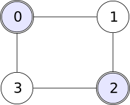
The doubled vertices form the separator \(S=\{0,2\}\). The cover sets are \(V_1=\{0,1,2\}\) and \(V_2=\{0,2,3\}\); their private vertices \(1,3\) have no connecting edge. The graph has only the 4 drawn edges, with no diagonal edge. Its precision is \[Q=\begin {pmatrix} 3&-1&0&-1\\-1&3&-1&0\\0&-1&3&-1\\-1&0&-1&3 \end {pmatrix}.\] Use \(V_1=(0,1,2)\), \(V_2=(0,2,3)\) and \(S=(0,2)\), with the listed coordinate orders. Each omitted vertex has precision \(3\), so the Schur formula gives \[\begin {aligned} \Lambda _1&=\begin {pmatrix} 8/3&-1&-1/3\\-1&3&-1\\-1/3&-1&8/3 \end {pmatrix},\\ \Lambda _2&=\begin {pmatrix} 8/3&-1/3&-1\\-1/3&8/3&-1\\-1&-1&3 \end {pmatrix},\\ \Lambda _S&=\begin {pmatrix}7/3&-2/3\\-2/3&7/3\end {pmatrix}. \end {aligned}\] Both triple laws have this same overlap marginal. Padding and subtracting gives \(Q\) entry by entry: each overlap diagonal is \(8/3+8/3-7/3=3\), and the induced overlap entry is \(-1/3-1/3+2/3=0\). The remaining edges retain weight \(-1\). The determinants are \(15,15,5\), respectively, so the glued normalization gives \(\det Q=15\cdot15/5=45\), agreeing with its eigenvalues \(1,3,3,5\). This uses one separator of a non-chordal cycle; it does not assert that arbitrary edge laws on that cycle glue.
Example 24.6. Compatible edge laws with no global extension [fdip-0067]AGENTDRAFTED
- November 1, 2026
Example 24.6. Compatible edge laws with no global extension [fdip-0067]AGENTDRAFTED
- November 1, 2026
On the four-cycle \(0,1,2,3,0\), prescribe centered Gaussian edge laws with unit variances and correlations \[\rho _{01}=\rho _{12}=\rho _{23}=\frac 9{10}, \qquad \rho _{30}=-\frac 9{10}.\] Each edge covariance has eigenvalues \(1/10,19/10\), hence is positive definite. All overlap singleton laws are \(N(0,1)\). Nevertheless there is no global positive-semidefinite covariance matrix with these entries, and therefore no global Gaussian extension.
Proof.
- November 1, 2026
Proof.
- November 1, 2026
In any joint law with these second moments, \[\|\phi _0-\phi _3\|_{L^2}=\sqrt {19/5}, \qquad \|\phi _i-\phi _{i+1}\|_{L^2}=\sqrt {1/5} \quad (i=0,1,2).\] But the first difference is the sum of the three consecutive differences. The triangle inequality would give \(\sqrt {19/5}\le 3\sqrt {1/5}\), contradicting \(19>9\). Any proposed positive-semidefinite covariance is a Gram matrix of real vectors and obeys the same norm inequality. Thus the obstruction already rules out semidefinite completion, without a nondegeneracy assumption.
The angular description gives another view of the same obstruction. Unit Gram vectors have consecutive angles \(\alpha =\arccos (9/10)\) and endpoint angle \(\pi -\alpha \). For unit vectors with successive angles \(\beta ,\gamma \) and \(\beta +\gamma \le \pi \), orthogonal decomposition along the middle vector and Cauchy–Schwarz give \[\langle u,w\rangle \ge \cos \beta \cos \gamma -\sin \beta \sin \gamma =\cos (\beta +\gamma ).\] Since arccosine decreases, the endpoint angle is at most \(\beta +\gamma \). If the sum exceeds \(\pi \), that bound is automatic. Iteration gives endpoint angle at most \(3\alpha \). But \(\alpha <\pi/4\), because \(9/10>1/\sqrt 2\); hence \(3\alpha <\pi -\alpha \), again a contradiction.
This example concerns the presheaf of laws on the edge cover: agreement on every overlap does not ensure existence. It is a concrete non-chordal obstruction of the kind distinguished by [grone1984positive, Theorem 7, p. 120]. It does not say that all data on a non-chordal graph fail to extend; the global four-cycle law in Example 24.5 supplies data that do extend.
Theorem 24.7. Chordal Gaussian gluing along a junction tree [fdip-0068]AGENTDRAFTED
- November 1, 2026
Theorem 24.7. Chordal Gaussian gluing along a junction tree [fdip-0068]AGENTDRAFTED
- November 1, 2026
A clique is a vertex subset whose distinct vertices are pairwise adjacent; a maximal clique is inclusion-maximal. A finite simple graph \(\Gamma \) on \(V\) is chordal if it has no induced cycle of length at least 4. Suppose centered positive-definite Gaussian laws \(\mu _K\) on its maximal cliques agree on every overlap. Then there is a unique centered positive-definite Gaussian law with these clique marginals that is Markov with respect to \(\Gamma \). Uniqueness is asserted within that Markov class.
The maximal cliques admit a junction tree: a tree \(\mathcal T\) whose nodes are the maximal cliques, such that the nodes containing any given vertex form a connected subtree. This is the running-intersection property. Write \(S_e=K\cap K'\) for the separator on an edge \(e=KK'\) and \(p_{S_e}\) for its common marginal density. Empty separators have density one. The glued law and precision are \[p(\phi )=\frac {\prod _Kp_K(\phi _K)} {\prod _{e\in E(\mathcal T)}p_{S_e}(\phi _{S_e})},\] \[Q=\sum _K\operatorname {pad}_K(\Lambda _K) -\sum _{e\in E(\mathcal T)} \operatorname {pad}_{S_e}(\Lambda _{S_e}).\] Separator terms are counted once per tree edge, including repetitions of the same vertex subset. For \(V=\varnothing \) the law is the unit mass and both products are empty.
Proof.
- November 1, 2026
Proof.
- November 1, 2026
We first justify the finite junction-tree construction. A vertex is simplicial when its neighbors form a clique. Every noncomplete chordal graph has two nonadjacent simplicial vertices. Here is an induction proof. In the connected case choose nonadjacent vertices \(a,b\) and an inclusion-minimal separator \(S\). Let \(C_a,C_b\) be their components in \(\Gamma \setminus S\). Minimality implies that each \(s\in S\) has a neighbor in both components: otherwise restoring that \(s\) would still leave \(a,b\) separated. If nonadjacent \(x,y\) belonged to \(S\), choose shortest \(x\)-to-\(y\) paths with internal vertices in \(C_a\) and in \(C_b\). Each path has no chord, and there are no edges between their interiors. Their union would be an induced cycle of length at least 4. Thus \(S\) is a clique.
Each induced graph \(C_a\cup S\) and \(C_b\cup S\) is smaller and chordal. If one is complete, any vertex in its component is simplicial. Otherwise induction gives two nonadjacent simplicial vertices; at most one lies in the clique \(S\), so choose one outside \(S\). Its full-graph neighbors still lie in that same induced graph, so it is simplicial in \(\Gamma \). The two choices are nonadjacent. In a disconnected graph choose a simplicial vertex in each of two components by the same induction; complete components pose no problem. Complete graphs have every vertex simplicial. This proves the assertion and allows repeated deletion of a simplicial vertex, a perfect elimination order.
Induct on that deletion to construct the clique tree. Remove a simplicial vertex \(v\), and write \(N\) for its neighbor clique. Unless no vertices remain, \(N\) lies in a maximal clique \(C\) of the remaining graph; when \(N=\varnothing \), choose any such \(C\). If \(N=C\), replace node \(C\) in its clique tree by \(C\cup \{v\}\). If \(N\subsetneq C\), attach \(N\cup \{v\}\) as a new leaf at \(C\). These are precisely the changes to the maximal cliques. In either case the nodes containing each old vertex remain connected, while \(v\) occurs only in the new node. A one-vertex graph starts the induction. Connecting different graph components in this way uses empty separators. This proves the required running-intersection property. The perfect-elimination characterization is also stated in [grone1984positive, Theorem 6, p. 119].
Now remove a leaf clique \(K\) of \(\mathcal T\) with neighbor \(C\) and separator \(S=K\cap C\). Running intersection says that \(A=K\setminus S\) occurs in no other clique, and that \(K\)'s intersection with the union of the remaining cliques is exactly \(S\). By induction glue the remaining clique laws; a one-clique tree starts with its prescribed law. The remaining law's marginal on \(S\) is the prescribed one, since it has the prescribed law on \(C\). The two-law theorem then glues in \(\mu _K\) by multiplication by \(p_K/p_S\). This proves normalization, positive definiteness, all clique marginals and the density formula. The precision formula follows at each step. Every nonzero summand is supported on a clique, so the precision is zero on all nonedges: the constructed law is Markov.
For uniqueness, \(S\) separates \(A\) from the remaining vertices outside \(S\): an edge out of \(A\) would belong to a maximal clique, but no other clique contains its endpoint in \(A\). Any Markov extension therefore factors across this separator by Theorem 24.3. Its marginal after removing \(A\) is again Markov for the induced remaining graph. Indeed the Schur correction from eliminating \(A\) is supported only on \(S\times S\), and \(S\) is a clique, so it creates no entry on a nonedge. Induction makes that remaining marginal unique; the separator factorization then makes the full law unique.
The positive-definite completion theorem of [grone1984positive, Theorem 7, p. 120, proof pp. 121–122] characterizes chordal graphs by existence for every compatible positive clique specification. The proof above additionally constructs the Markov extension and proves uniqueness within that class. Bare completion existence alone does not assert that all extensions are identical. Even for two isolated vertices, Example 24.2 has many positive completions and exactly one Markov completion.
Remark 24.8. What the gluing theorem establishes about descent [fdip-0069]AGENTDRAFTED
- November 1, 2026
Remark 24.8. What the gluing theorem establishes about descent [fdip-0069]AGENTDRAFTED
- November 1, 2026
The presheaf of Gaussian laws has an explicit domain, restriction maps and overlap compatibility. On the finite-subset poset with covers given by unions, it is not a sheaf: the two-singleton cover has non-unique extensions, and the four-cycle edge cover has compatible data with no extension. These are separate failures of uniqueness and existence.
The chordal theorem gives a precise replacement on a specified clique cover. It chooses the unique extension satisfying that graph's Markov condition and supplies its density and precision. A different graph or a different collection of local laws is a different problem. This does not turn fixed-graph Markov laws into a presheaf closed under every marginal restriction; Schur elimination can introduce precision edges.
The earlier factorization comparison separates scalar factorization, functorial factorization, localization and descent. The present result adds a concrete finite local-to-global theorem for laws, but no descent data for the objects and arrows of the background groupoid. A stack would require a specified site, a category fibred over it, sheaves of morphisms and effective object descent [stacks2017stacks, Definition 8.4.1], Tag 0268. No such stack assertion follows from the density gluing formula; stack-level gluing of background objects remains an additional question.
25. Connections, holonomy and twisted operators [fdip-006C]AGENTDRAFTED
- November 1, 2026
25. Connections, holonomy and twisted operators [fdip-006C]AGENTDRAFTED
- November 1, 2026
If local field frames can differ, how are neighboring values compared? An ordinary edge difference compares two values in the same field space. A connection first transports one endpoint value to the other. The resulting positive precision depends on this extra background data. Changing frames at the vertices changes its matrix by an isometry; transport around a cycle retains information that vertex frames cannot remove.
A spanning tree reduces this information to finitely many holonomies. For a complex line on a cycle, the determinant can then be computed exactly. A nontrivial twist can remove the constant zero mode, and the normalized complex Gaussian gives an explicit holonomy action on a supplied circle. Antiperiodic spatial differences provide a related example: exact kernel dimensions change, while the additional low-energy branches of the centered symbol remain.
Definition 25.1. A connection background and its positive precision [fdip-006D]AGENTDRAFTED
- November 1, 2026
Definition 25.1. A connection background and its positive precision [fdip-006D]AGENTDRAFTED
- November 1, 2026
Fix a finite or compact Hausdorff group \(G\) and a finite-dimensional real or complex representation \(\rho :G\to \operatorname {GL}(F)\), continuous in the compact case. Supply a positive inner product for which \(\rho \) is orthogonal or unitary. If necessary, start from any positive inner product and average it: \[\langle x,y\rangle _G =\int _G\langle \rho (g)x,\rho (g)y\rangle _0\,dg.\] Here \(dg\) is normalized right Haar measure; for a finite group it is the uniform average. Haar existence and inversion from left to right are given in [gleason2010haar, Theorem 4.3, pp. 6–9; Proposition 4.1, pp. 4–5]. Compactness makes its nonzero total mass finite, allowing normalization. Right invariance gives invariance of the displayed pairing. The integrand is continuous and strictly positive for \(x=y\ne 0\), so the average is positive. The invariant metric is part of the data used below.
On a finite incidence presentation, a connection assigns \(U_e\in G\) to every chosen oriented edge. Reversing that edge assigns \(U_{\bar e}=U_e^{-1}\). Set \(H=F^V\) and \(K=F^E\), with the sums of the supplied fiber inner products. Write \(U_e\) also for \(\rho (U_e)\) in operator formulas. For scalar weights \(w_e>0\) and mass \(m>0\), define \[\begin {aligned} (d_Uf)(e)&=f(h(e))-U_ef(s(e)),\\ W&=\operatorname {diag}(w_eI_F),\\ L_U&=d_U^*Wd_U,\qquad Q_U=L_U+m^2I_H. \end {aligned}\] The adjoint uses these declared inner products. Directly, \[\langle f,Q_Uf\rangle =\sum _e w_e\|f(h(e))-U_ef(s(e))\|^2+m^2\|f\|^2.\] Thus \(Q_U\ge m^2I_H>0\). This is the unitary connection version of the difference energy; the adjoint qualification is also explicit in [kenyon2011spanning, Section 3.3, p. 6].
At \(m=0\), the same sum shows \[\ker L_U=\ker d_U =\{f:f(h(e))=U_ef(s(e))\text { for every }e\}.\] Its elements are called parallel sections. The unpinned massless Gaussian is normalizable exactly when this space is zero: then \(L_U\) is positive definite; otherwise the density is constant along a nonzero kernel direction and its integral diverges. This is separate from the pinned construction. Nontrivial group holonomy need not eliminate all parallel vectors in a higher-dimensional or nonfaithful representation.
Mathlib's LinearMap.ker_adjoint_comp_self gives
\(\ker (A^*A)=\ker A\) for finite-dimensional inner-product spaces.
Apply it to \(A=W^{1/2}d_U\); positive weights make \(W^{1/2}\)
invertible. This supports the kernel identity, not the connection,
holonomy or normalizability assertions.
Proposition 25.2. Gauge covariance and transport of selected laws [fdip-006E]AGENTDRAFTED
- November 1, 2026
Proposition 25.2. Gauge covariance and transport of selected laws [fdip-006E]AGENTDRAFTED
- November 1, 2026
For a connection background, the gauge group \(G^V\) changes the frame independently at each vertex. For \(g=(g_v)_{v\in V}\), define \[\begin {aligned} (gU)_e&=g_{h(e)}U_eg_{s(e)}^{-1},\\ (G_Vf)_v&=\rho (g_v)f_v,\\ (G_Ea)_e&=\rho (g_{h(e)})a_e. \end {aligned}\] Then \[\begin {aligned} d_{gU}G_V&=G_Ed_U,\\ Q_{gU}&=G_VQ_UG_V^{-1},\\ \det Q_{gU}&=\det Q_U. \end {aligned}\] In particular, the massive spectra and Gaussian normalizers are gauge invariant.
Proof.
- November 1, 2026
Proof.
- November 1, 2026
On an edge with endpoints \(s,h\), \[\begin {aligned} (d_{gU}G_Vf)(e) &=\rho (g_h)f_h-\rho (g_hU_eg_s^{-1})\rho (g_s)f_s\\ &=\rho (g_h)(f_h-\rho (U_e)f_s). \end {aligned}\] This proves the first identity. Both \(G_V\) and \(G_E\) are isometries, and scalar weights imply \(G_E^*WG_E=W\). Taking adjoints in \(d_{gU}=G_Ed_UG_V^{-1}\) therefore gives \[d_{gU}^*Wd_{gU}=G_Vd_U^*Wd_UG_V^{-1}.\] The mass term commutes with \(G_V\). Multiplicativity of the determinant gives its invariance. The same isometry preserves real Euclidean volume, or the real volume underlying a complex Hermitian space, so changing variables also preserves the corresponding Gaussian integral.
For a fixed incidence presentation, \(U\mapsto gU\) is a group action: \(g_2(g_1U)=(g_2g_1)U\). Its action groupoid has connections as objects and gauge transformations as arrows. If a selector is included, use an orthogonal projector \(P\) on real \(H\), or a complex-linear orthogonal projector on complex \(H\), and transport it by \[P'=G_VPG_V^{-1}.\] The identity, composition and inverse obey this equation by conjugation. Together with relabelings that carry the connection values, these are the connection counterparts of selected-background arrows. The earlier scalar backgrounds and relabeling arrows are recovered with \(F=\mathbb R\), \(G=\{1\}\) and their original selector rank condition.
On the selected space \(X=\operatorname {im}P\), the compressed inverse is \(C_P=(PQ_U^{-1}P)|_X\). The restriction \(G_X:X\to \operatorname {im}P'\) satisfies \[C_{P'}=G_XC_PG_X^{-1}.\] Indeed insert the three conjugation identities for \(P'\), \(Q_{gU}^{-1}\) and \(P'\). Inversion transports the selected precision. For real fields this is exactly the selected Gaussian transport; for complex fields the Gaussian convention is specified in Example 25.6.
Unitarity is essential for this argument. A nonorthogonal matrix representation with an unchanged Euclidean metric need not satisfy \(G_E^*WG_E=W\); changing connection matrices alone would then fail to produce the asserted conjugacy.
Theorem 25.3. Graph connections are classified by holonomy [fdip-006F]AGENTDRAFTED
- November 1, 2026
Theorem 25.3. Graph connections are classified by holonomy [fdip-006F]AGENTDRAFTED
- November 1, 2026
Let \(\Gamma \) be a finite connected graph with chosen edge orientations and root \(o\). For a path traversing \(e_1,\ldots ,e_k\), use inverse edge values when traversing backwards and define its holonomy by \[U_{e_k}\cdots U_{e_1}.\] Thus the rightmost factor transports first. Use the same composition convention for loops: \(\beta \alpha \) first traverses \(\alpha \) and then \(\beta \). The gauge classes of \(G\)-valued connections are \[\operatorname {Hom}(\pi _1(\Gamma ,o),G)/G \;\cong \;G^{b_1}/G,\qquad b_1=|E|-|V|+1,\] where \(G\) acts by simultaneous conjugation. The second identification depends on a spanning tree and orientations of the remaining edges. This classifies group-valued connections, not their possibly nonfaithful representation images or the spectra of their precisions.
Proof.
- November 1, 2026
Proof.
- November 1, 2026
Choose a spanning tree \(T\). Each vertex \(v\) has a unique tree path from \(o\); let \(t_v\in G\) be its transport, with \(t_o=1\). Use the gauge \(g_v=t_v^{-1}\). If a tree edge runs from \(s\) to \(h\), its path transports satisfy \(t_h=U_et_s\), with the equivalent inverse identity when the rooted path traverses the edge backwards. Hence \[(gU)_e=t_h^{-1}U_et_s=1\qquad (e\in T).\] Every connection therefore has a representative with all tree values one. The remaining \(|E|-|T|=b_1\) edge values are unrestricted.
A gauge transformation carrying one such representative to another satisfies \(g_hg_s^{-1}=1\) on every tree edge. Tree connectivity forces all \(g_v\) to equal one element \(a\in G\). It conjugates every remaining edge value by \(a\). Conversely every simultaneous conjugation comes from this constant gauge. This proves the classification by \(G^{b_1}/G\), including the case of a tree, where \(b_1=0\).
Traversing a path and then its inverse gives cancelling group factors, so transport is unchanged by removing backtracking. The loops that run from \(o\) through the tree to the source of a non-tree edge, traverse it and return through the tree are a free basis of \(\pi _1(\Gamma ,o)\). This is [hatcher2002algebraic, Proposition 1A.2 and its proof, pp. 84–85]: contract the tree to obtain a wedge of \(b_1\) circles. Assigning arbitrary values to this free basis gives every group homomorphism. In tree gauge these values are precisely the non-tree edge values. A general gauge conjugates each rooted loop holonomy by \(g_o\), proving the first identification as well.
With two-cells attached, call a connection flat when the ordered holonomy around every attaching boundary is the identity in \(G\). Equivalently the graph homomorphism kills the normal subgroup generated by those boundaries. It therefore factors through the fundamental group of the resulting space. A representation \(\rho \) can send a nonidentity group element to the identity operator; operator flatness alone is therefore insufficient when \(\rho \) is nonfaithful.
In the representation on \(F\), a parallel section is determined by its root value \(x\in F\). Tree transport defines its other values, and each non-tree edge condition says that its rooted holonomy fixes \(x\). Consequently evaluation at \(o\) identifies the space of parallel sections with the common fixed space of the holonomy representation. This proves the massless-kernel criterion of Definition 25.1 in terms of cycle data.
Theorem 25.4. Determinants of a twisted cycle [fdip-006G]AGENTDRAFTED
- November 1, 2026
Theorem 25.4. Determinants of a twisted cycle [fdip-006G]AGENTDRAFTED
- November 1, 2026
Let \(C_n\), \(n\ge 3\), have vertices \(0,\ldots ,n-1\) and edges \(j\to j+1\) modulo \(n\). Take a complex line with unitary connection, positive weights \(w_j\), and total oriented holonomy \(u=\prod _jU_j=e^{i\theta }\). For \(L_\theta =d_U^*Wd_U\), \[\det L_\theta =\left (\prod _jw_j\right )(2-2\cos \theta ).\] For unit weights and \(c\ge 0\), let \(\omega \ge 0\) be determined by \(2\cosh \omega =2+c\). Then \[\det (cI+L_\theta )=2\cosh (n\omega )-2\cos \theta .\] The first formula is the cycle case of the weighted line-bundle matrix-tree formula, [kenyon2011spanning, Theorem 5, Section 7.1, p. 13]. Its unweighted precursor is [kenyon2011spanning, Theorem 1, p. 7]. Both cycle identities are proved directly below.
Proof.
- November 1, 2026
Proof.
- November 1, 2026
Use Theorem 25.3 to set \(U_0=\cdots =U_{n-2}=1\) and \(U_{n-1}=u\). The square incidence matrix has row equations \(f_{j+1}-f_j\) for \(j<n-1\) and \(f_0-uf_{n-1}\) for the last row. In its determinant expansion the only nonzero permutations choose all source entries or all head entries: choosing one head entry forces the next row to choose its head entry, and so around the cycle. Their signed sum is \(1-u\) up to an overall sign. Hence \[\det (d_U^*Wd_U) =|\det d_U|^2\det W =|1-u|^2\prod _jw_j.\] Since \(|1-e^{i\theta }|^2=2-2\cos \theta \), this proves the first formula, including trivial holonomy.
For unit weights introduce the unitary shift \[(T_\theta f)_j=\begin {cases} f_{j+1},&j<n-1,\\ u^{-1}f_0,&j=n-1. \end {cases}\] The last edge difference is \(u(T_\theta f-f)_{n-1}\), so its modulus is unchanged. Thus \(L_\theta =2I-T_\theta -T_\theta ^*\). The seam convention is \(f_n=u^{-1}f_0\); its modes and eigenvalues are \[\begin {aligned} p_k&=(2\pi k-\theta )/n,\qquad 0\le k<n,\\ f_k(j)&=n^{-1/2}e^{ip_kj},\\ L_\theta f_k&=(2-2\cos p_k)f_k. \end {aligned}\] Distinct modes are orthogonal because their ratios are nontrivial \(n\)-th roots of unity; the finite geometric sum vanishes. There are \(n\) modes, so they form a complete basis.
Put \(r=e^\omega \) and \(z_k=e^{ip_k}\). The numbers \(z_k\) are all roots of \(z^n=u^{-1}\). Since \[c+2-z-z^{-1}=r^{-1}(r-z)(r-z^{-1}),\] the product of the eigenvalues is \[\begin {aligned} \det (cI+L_\theta ) &=r^{-n}(r^n-u^{-1})(r^n-u)\\ &=r^n+r^{-n}-u-u^{-1}\\ &=2\cosh (n\omega )-2\cos \theta . \end {aligned}\] The computation remains valid at \(c=0\), when \(r=1\).
Example 25.5. An antiperiodic four-cycle has no parallel line section [fdip-006H]AGENTDRAFTED
- November 1, 2026
Example 25.5. An antiperiodic four-cycle has no parallel line section [fdip-006H]AGENTDRAFTED
- November 1, 2026
Give the unit four-cycle total holonomy \(u=-1\), or \(\theta =\pi \). In the tree gauge, three links are one and the final link is minus one. The cycle modes have momenta \(-\pi /4,\pi /4,3\pi /4,5\pi /4\), so \[\operatorname {spec}L_\pi =\{2-\sqrt 2,2-\sqrt 2,2+\sqrt 2,2+\sqrt 2\}.\] All 4 eigenvalues are positive, and \(\det L_\pi =((2-\sqrt 2)(2+\sqrt 2))^2=4\).

The arrows show the chosen orientation; labels are connection values, not edge weights, which are all one. The thick edge carries the remaining holonomy after the other three form a tree. A parallel section would have \(f_0=f_1=f_2=f_3\) along those tree edges and \(f_0=-f_3\) along the last edge, forcing zero. Thus the massless complex Gaussian exists without a pin. With trivial holonomy the constant line is a kernel instead. This is a change of background connection, distinct from conditioning a scalar Gaussian on pinned values.
Example 25.6. A normalized complex holonomy action on the circle [fdip-006I]AGENTDRAFTED
- November 1, 2026
Example 25.6. A normalized complex holonomy action on the circle [fdip-006I]AGENTDRAFTED
- November 1, 2026
Use the supplied unit-circle mesh, now with complex fields and total holonomy \(e^{i\theta }\). On \(\mathbb C^n\), take \[\langle z,w\rangle _n=\frac 1n\sum _j\overline {z_j}w_j, \qquad Q_{n,\theta }=n^2L_\theta +\mu I,\qquad \mu >0.\] Here \(L_\theta \) is the unit-weight twisted cycle, \(n\ge 3\), and the same factor \(n^2\) fixes the circle length scale. Let \(d\operatorname {vol}_n\) be the real volume induced by this Hermitian pairing. If \(z_j=x_j+iy_j\), then \[d\operatorname {vol}_n=n^{-n}\prod _jdx_j\,dy_j.\] Indeed \(z\mapsto z/\sqrt n\) is an orthonormal coordinate change in complex dimension \(n\), hence real dimension \(2n\).
Choose the complex Gaussian convention \[\begin {aligned} Z_n(\theta )&=\pi ^{-n}\int _{\mathbb C^n} e^{-\langle z,Q_{n,\theta }z\rangle _n} \,d\operatorname {vol}_n(z),\\ W_n(\theta )&=-\log Z_n(\theta ). \end {aligned}\] Unitary diagonalization gives one factor per eigenvalue \(\lambda >0\). Polar coordinates evaluate it: \[\begin {aligned} \pi ^{-1}\int _{\mathbb R^2}e^{-\lambda (x^2+y^2)}dx\,dy &=2\int _0^\infty e^{-\lambda r^2}r\,dr\\ &=\lambda ^{-1}. \end {aligned}\] Therefore \[Z_n(\theta )=(\det _{\mathbb C}Q_{n,\theta })^{-1}, \qquad W_n(\theta )=\log \det _{\mathbb C}Q_{n,\theta }.\] This complex convention has no factor \(1/2\) in the determinant action; the earlier real Gaussian action uses a different exponent and real field dimension.
Since \(Q_{n,\theta }=n^2(L_\theta +\mu n^{-2}I)\), define the explicitly subtracted finite action by \[\widetilde W_n(\theta )=W_n(\theta )-2n\log n.\] The cycle determinant gives \[\begin {aligned} \widetilde W_n(\theta ) &=\log (2\cosh (n\omega _n)-2\cos \theta ),\\ 2\cosh \omega _n&=2+\mu /n^2,\qquad \omega _n\ge 0. \end {aligned}\] Thus the removed term is independent of holonomy; it is part of the stated normalization, not a finite determinant omitted from the formula.
The identity \(\cosh \omega -1=2\sinh ^2(\omega /2)\) gives \(\omega _n=2\operatorname {arsinh}(\sqrt {\mu }/(2n))\). For \(t>0\), integrate the derivative \((\operatorname {arsinh}t)'=(1+t^2)^{-1/2}\) to obtain \[\frac 1{\sqrt {1+t^2}} \le \frac {\operatorname {arsinh}t}{t}\le 1.\] Consequently \(n\omega _n\to \sqrt \mu \). The positive limiting argument of the logarithm is at least \(2\cosh \sqrt \mu -2>0\), so \[\widetilde W_n(\theta )\longrightarrow W(\theta )=\log (2\cosh \sqrt \mu -2\cos \theta ).\] This is a direct limit of the normalized finite determinants, beyond the separate fixed-mode comparison; no interchange of an infinite product is used.
For \(\mu >0\), \(W(\theta )\) is minimized exactly at trivial holonomy \(\theta =0\) modulo \(2\pi \), since \(\cos \theta \le 1\). Equivalently the integrated matter factor \(e^{-W}\) is largest there. At \(\mu =0\) and nontrivial holonomy the same finite calculation gives \(W(\theta )=\log (2-2\cos \theta )\). At trivial holonomy there is a zero mode: the unpinned Gaussian integral diverges and this determinant action is undefined. Its formal logarithm of zero is not a normalized Gaussian action. The circle, its scale and the connection remain supplied data.
Example 25.7. Antiperiodic spatial Dirac modes [fdip-006J]AGENTDRAFTED
- November 1, 2026
Example 25.7. Antiperiodic spatial Dirac modes [fdip-006J]AGENTDRAFTED
- November 1, 2026
Keep the spatial Clifford module \(S=(\mathbb C^2)^{\otimes d}\), with \(\dim _{\mathbb C}S=2^d\), and periods \(N_j\ge 3\). Give scalar fields on the fundamental box \(0\le x_j<N_j\) the antiperiodic extension \[f(x+N_je_j)=-f(x)\qquad (1\le j\le d).\] The forward shift \(T_j^-\) uses this extension at a seam. It is a signed permutation, hence unitary in the counting pairing; shifts in different coordinates commute. They act on the lattice factor only, so they commute with the Clifford matrices on \(S\). Define \[D^- =\sum _{j=1}^d\gamma _j\otimes \frac {T_j^--(T_j^-)^{-1}}2.\] These are fixed flat line twists, each with holonomy minus one.
For labels \(0\le r_j<N_j\), set \[p_j=\frac {(2r_j+1)\pi }{N_j},\qquad \chi _r(x)=\left (\prod _jN_j\right )^{-1/2} e^{i\sum _jp_jx_j}.\] The exponential obeys the declared antiperiodic extension. Differences of two allowed momenta are periodic Fourier momenta, so the same geometric-sum proof as Theorem 16.2 makes these functions a complete orthonormal basis of fields on the box. On its momentum block, \[\begin {aligned} D^-(p)&=i\sum _j\gamma _j\sin p_j,\\ -D^-(p)^2&=\left (\sum _j\sin ^2p_j\right )I_S. \end {aligned}\] The square follows from the Clifford anticommutators and commuting coordinate shifts, exactly as in the untwisted calculation.
A block is zero precisely when every \(\sin p_j=0\); otherwise its inverse is \(-D^-(p)/(\sum _j\sin ^2p_j)\). Since \(0<p_j<2\pi \), the only possible zero is \(p_j=\pi \), which requires \(2r_j+1=N_j\). It occurs once when \(N_j\) is odd and never when it is even. Hence \[\dim _{\mathbb C}\ker D^-= \begin {cases} 2^d,&\text {all periods are odd},\\ 0,&\text {at least one period is even}. \end {cases}\] For two directions the comparison with Proposition 16.3 is \[\begin {array}{c|ccc} (N_1,N_2)&(4,4)&(4,3)&(3,3)\\\hline \dim \ker D&16&8&4\\ \dim \ker D^-&0&0&4 \end {array}\] These are dimensions in the specified reducible module, not physical species or chirality counts.
The twist changes exact zeros without removing the centered symbol's extra low-energy branches. For large \(N_j\), an allowed momentum lies within \(\pi /N_j\) of each corner coordinate \(0\) or \(\pi \), with distance to \(0\) understood modulo \(2\pi \). Thus \(|\sin p_j|\le \pi /N_j\) near every such corner. After restoring a fixed-length mesh spacing \(a_j=L_j/N_j\), the corresponding \(|\sin p_j|/a_j\) is bounded by \(\pi /L_j\); branches near the \(\pi \) corners remain at finite energy alongside the branch near zero. This does not say that the rescaled antiperiodic eigenvalues tend to zero at fixed circle lengths. The additional branches are the centered-difference doubling problem, whose sine symbol is discussed in [wingate2025lattice, Section 9.1, Equations (9.6)–(9.7), p. 20]. A boundary twist alone does not supply its Wilson-operator remedy.
Remark 25.8. Fixed connections and dynamical fields [fdip-006K]AGENTDRAFTED
- November 1, 2026
Remark 25.8. Fixed connections and dynamical fields [fdip-006K]AGENTDRAFTED
- November 1, 2026
A connection in this chapter is fixed background data. Gauge transformations compare its descriptions; taking their quotient does not prescribe a probability law on connections. The holonomy action integrates matter while retaining the connection as a parameter. To make the connection dynamical one must also specify its integration measure and action, and then integrate or sum over connection configurations.
The earlier induced action on weighted graphs likewise keeps the weights fixed. One could subsequently promote them to integration variables, but that is an additional model choice. Neither the fixed-weight action nor the present connection construction makes weights dynamical or supplies gravitational dynamics. A prescribed circle limit and a twisted spatial Dirac operator also do not supply a time direction, reflection positivity or Lorentzian reconstruction. These distinctions remain part of the open physical interfaces.
26. Finite gauge fields and an exact torus law [fdip-006L]AGENTDRAFTED
- November 1, 2026
26. Finite gauge fields and an exact torus law [fdip-006L]AGENTDRAFTED
- November 1, 2026
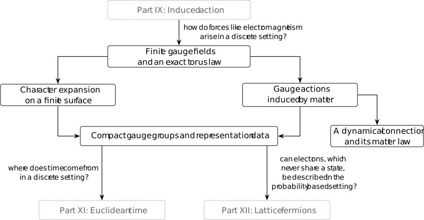
How can the transports used to compare neighboring fields themselves fluctuate? A connection background assigns a fixed transport to each edge; it is already gauge-field data. A law on those transports makes them dynamical. We now sum over them as field variables, while keeping the graph, its square faces and the group fixed. The faces are extra incidence data: the earlier graph alone does not specify them. A chosen unitary representation gives a Wilson action and a finite probability law with an explicit counting-measure convention.
Matter integration already distinguishes connections in the massive complex Gaussian on a supplied circle. Its normalized holonomy action \(W\) is minimized at trivial holonomy, so the integrated matter factor \(e^{-W}\) is largest there. That comparison leaves the circle and connection supplied. The finite law here is a further choice; transport alone does not derive a force such as electromagnetism.
Gauge averaging first determines which parts of an observable can contribute to its expectation. For the two-element group on a square torus, all plaquette signs can then be counted exactly. One global constraint and two remaining cycle holonomies account for the partition function's normalization. The resulting loop formula gives a pure-gauge area law in two dimensions; no matter field is included in that result.
Definition 26.1. Square faces on a finite graph [fdip-006M]AGENTDRAFTED
- November 1, 2026
Definition 26.1. Square faces on a finite graph [fdip-006M]AGENTDRAFTED
- November 1, 2026
A finite cubical 2-complex, in the square-cell convention used here, consists of a finite incidence presentation \((V,E,s,h)\), a finite set \(\mathcal P\) of squares, and a specified four-edge attaching walk for each square. Choose one orientation for each edge and one boundary orientation and starting vertex for each square. Its walk is \[\partial p=(e_{p,1}^{\epsilon _{p,1}},\ldots , e_{p,4}^{\epsilon _{p,4}}),\qquad \epsilon _{p,j}\in \{1,-1\},\] where an exponent \(-1\) means traversal against the chosen edge orientation. Consecutive endpoints match, including the last to the first.
Starting from the one-dimensional realization, attach one copy of \([0,1]^2\) for each \(p\), mapping its 4 sides to the specified traversed edges, and use the quotient topology. Boundary vertices or sides may be identified in this presentation, as in periodic quotients; no regularity or nonpositive-curvature condition is imposed. No higher-dimensional cubes are supplied. The squares and their attaching maps are additional data, just as the filled face is additional data in the triangle comparison.
The main example is the square torus with periods \(N_1,N_2\ge 3\). Its vertices are \[V=(\mathbb Z/N_1\mathbb Z)\times (\mathbb Z/N_2\mathbb Z).\] There are horizontal edges \(a_{x,y}:(x,y)\to (x+1,y)\) and vertical edges \(b_{x,y}:(x,y)\to (x,y+1)\), with indices read modulo the periods. The square at \((x,y)\) has boundary walk \[a_{x,y}\,b_{x+1,y}\,a_{x,y+1}^{-1}\,b_{x,y}^{-1}.\] This written order is the order of traversal. Put \[n=|V|=N_1N_2,\qquad |E|=2n,\qquad P=|\mathcal P|=n.\] The realization is the usual square grid on a torus. The periods ensure that each square has 4 distinct vertices and sides, although periodic identifications occur globally.
Definition 26.2. Plaquette transport and Wilson loops [fdip-006N]AGENTDRAFTED
- November 1, 2026
Definition 26.2. Plaquette transport and Wilson loops [fdip-006N]AGENTDRAFTED
- November 1, 2026
Let \(G\) be a finite group on a square complex. A connection is \(U\in G^E\), with \(U_{\bar e}=U_e^{-1}\) on a reversed edge. For a traversed path \(C=(e_1^{\epsilon _1},\ldots ,e_k^{\epsilon _k})\), define \[U_C=U_{e_k}^{\epsilon _k}\cdots U_{e_1}^{\epsilon _1}.\] The first transport acts on the right. The plaquette holonomy is \(U_p=U_{\partial p}\). The gauge group \(\mathcal G=G^V\) acts by \[(gU)_e=g_{h(e)}U_eg_{s(e)}^{-1}.\] Cancellation at successive vertices gives \[(gU)_C=g_{h(C)}U_Cg_{s(C)}^{-1}.\] For a closed path based at \(v\), this is conjugation by \(g_v\).
Choose a unitary representation \(\rho :G\to U(d)\) with \(d>0\), and let \(\chi _\rho (g)=\operatorname {Tr}\rho (g)\) be its character. The Wilson loop of a closed path is the unnormalized trace \[W_\rho (C)=\chi _\rho (U_C).\] It is gauge invariant. Changing the starting vertex conjugates the holonomy, so it does not change this trace. Reversing the path replaces \(U_C\) by \(U_C^{-1}\), hence replaces \(W_\rho (C)\) by its complex conjugate. In particular \(\operatorname {Re}W_\rho (C)\) is independent of the chosen boundary orientation. These are the transport and trace conventions of [wingate2025lattice, equations (6.14)–(6.19), pp. 7–8].
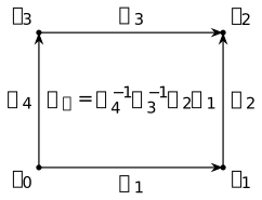
The arrows show the chosen edge orientations and the labels are connection values, not scalar weights. The boundary traversal is \[v_0\to v_1\to v_2\to v_3\to v_0.\] It uses the top and left edges backwards, accounting for both inverses.
Definition 26.3. The finite Wilson action and counting law [fdip-006O]AGENTDRAFTED
- November 1, 2026
Definition 26.3. The finite Wilson action and counting law [fdip-006O]AGENTDRAFTED
- November 1, 2026
For the finite connection data and a fixed real \(\beta \ge 0\), define the Wilson action \[S_W(U)=\beta \sum _{p\in \mathcal P} \left (1-\frac {\operatorname {Re}\chi _\rho (U_p)}d\right ).\] Since \(\rho (U_p)\) is unitary, its eigenvalues have modulus one and \(-d\le \operatorname {Re}\chi _\rho (U_p)\le d\). Thus \(S_W(U)\ge 0\). The action is gauge invariant and does not depend on starting vertices or boundary orientations.
Use unnormalized counting measure on each edge group, and therefore on \(G^E\). The partition function, probability and expectation are \[\begin {aligned} Z_W&=\sum _{U\in G^E}e^{-S_W(U)},\\ \mathbb P_W(U)&=Z_W^{-1}e^{-S_W(U)},\\ \langle F\rangle _W&=Z_W^{-1}\sum _{U\in G^E}F(U)e^{-S_W(U)}. \end {aligned}\] These finite sums have \(0<Z_W<\infty \). Matrix-valued observables are averaged entry by entry. The finite group and chosen representation are inputs to this law, alongside the square complex and \(\beta \).
The constant term in the action matters for the partition function. With \(P=|\mathcal P|\), put \[\begin {aligned} \mathcal Z(\beta ) &=\sum _{U\in G^E}\exp \left ( \frac \beta d\sum _p\operatorname {Re}\chi _\rho (U_p)\right ),\\ Z_W(\beta )&=e^{-\beta P}\mathcal Z(\beta ). \end {aligned}\] The two weights define the same normalized expectation. Replacing each edge's counting measure by uniform probability measure instead gives \(|G|^{-|E|}Z_W\); that is a different partition-function normalization, again with the same expectation. In particular \(Z_W(0)=|G|^{|E|}\). The action and expectation agree with the conventions in [wingate2025lattice, equations (6.20)–(6.21), p. 8]; that source uses normalized Haar integration for its compact-group setting, whereas the finite counting convention here is explicit.
Theorem 26.4. Finite gauge averaging [fdip-006P]AGENTDRAFTED
- November 1, 2026
Theorem 26.4. Finite gauge averaging [fdip-006P]AGENTDRAFTED
- November 1, 2026
For the finite Wilson law, define \[(\mathcal AF)(U)=\frac 1{|\mathcal G|} \sum _{g\in \mathcal G}F(gU),\qquad \mathcal G=G^V.\] Then \(\mathcal A\) projects onto gauge-invariant observables and \[\langle F\rangle _W=\langle \mathcal AF\rangle _W.\] In particular \(\langle F\rangle _W=0\) whenever \(\mathcal AF=0\). A general noninvariant observable may have a nonzero invariant part; only \(F-\mathcal AF\) is always forced to have zero expectation.
Proof.
- November 1, 2026
Proof.
- November 1, 2026
For each \(g\), the map \(U\mapsto gU\) is a bijection of \(G^E\) with inverse \(U\mapsto g^{-1}U\). Gauge invariance of the action and change of variable in a finite sum give \[\sum _U F(gU)e^{-S_W(U)}=\sum _U F(U)e^{-S_W(U)}.\] Divide by \(Z_W\) and average over \(g\). Reindexing \(g\mapsto gh\) gives \((\mathcal AF)(hU)=(\mathcal AF)(U)\). If \(F\) is already invariant then \(\mathcal AF=F\), proving \(\mathcal A^2=\mathcal A\) and the asserted range.
Let \(\sigma \) be a nontrivial irreducible complex representation of \(G\), and let \(e\) have distinct endpoints. Then \[\langle \sigma (U_e)\rangle _W=0.\] To see this, set \(R=|G|^{-1}\sum _{a\in G}\sigma (a)\). Reindexing shows that \(\sigma (b)R=R\) for every \(b\), so \(R\) maps into the fixed-vector space. It is the identity on that space. A nonzero fixed vector would span a trivial subrepresentation; irreducibility and nontriviality therefore make the fixed-vector space zero and \(R=0\). Averaging the gauge transformation at \(h(e)\) while fixing the other vertices now replaces \(\sigma (U_e)\) by \(R\sigma (U_e)=0\). The expectation is unchanged by this averaging, by the same finite change-of-variable proof. Distinct endpoints are essential here.
For a self-loop, the transformation is only conjugation. The one-loop example shows that its expectation need not vanish.
This is a direct finite averaging proof, related to
Maschke averaging. Mathlib's
Representation.isProj_averageMap proves projection onto
invariants for a finite group representation over a commutative ring
in which the group order is invertible. Over \(\mathbb C\), apply it
to the inverse-pullback representation
\((R_gF)(U)=F(g^{-1}U)\), or to \(\sigma \) above. This supports the
linear averaging step, not the Wilson probability or torus formulas.
Example 26.5. A self-loop with nonzero expectation [fdip-006T]AGENTDRAFTED
- November 1, 2026
Example 26.5. A self-loop with nonzero expectation [fdip-006T]AGENTDRAFTED
- November 1, 2026
For a self-loop \(e\), the transformation is only conjugation. In the square-cell convention, take one vertex, one loop and one square whose attaching walk traverses that loop 4 times. Use the finite Wilson law. With \(G=\{1,\omega ,\omega ^2\}\) and \(\omega =e^{2\pi i/3}\), use the one-dimensional representation \(\rho (U)=U\). Then \(U_p=U^4=U\), the gauge action is trivial, and \[\langle U\rangle _W =\frac {1-e^{-3\beta/2}}{1+2e^{-3\beta/2}}>0\qquad (\beta >0).\] Thus no general open-edge vanishing conclusion extends to self-loops.
Lemma 26.6. Plaquette signs and the two torus holonomies [fdip-006Q]AGENTDRAFTED
- November 1, 2026
Lemma 26.6. Plaquette signs and the two torus holonomies [fdip-006Q]AGENTDRAFTED
- November 1, 2026
On the square torus, let \(G=\mathbb Z_2=\{1,-1\}\) under multiplication, with \(n=|V|=P\) and \(|E|=2n\). The map sending a connection to its plaquette signs has image exactly \[\left \{(u_p)\in \{1,-1\}^{\mathcal P}:\prod _pu_p=1\right \}.\] Every such sign configuration has \(2^{n+1}\) preimages in \(G^E\). It consists of 4 gauge orbits, distinguished by two fundamental cycle holonomies.
Proof.
- November 1, 2026
Proof.
- November 1, 2026
Each edge occurs twice among the square boundaries, so \(\prod _pU_p=1\). Conversely, choose a spanning tree in the connected dual graph, whose vertices are squares and whose edges cross their shared primal edges. Root this tree and set all primal edge signs to \(1\). Process dual leaves towards the root. At each leaf, its unique remaining dual-tree edge crosses a primal edge shared with its parent. Flip that primal sign exactly when needed to give the leaf its prescribed plaquette sign, then remove the leaf. This changes only the leaf and its parent among the unprocessed squares and changes no previously fixed square. At the last square, the global product constraint forces the prescribed root sign. This constructs every even-parity plaquette pattern.
The plaquette map is a homomorphism between finite abelian groups. Multiplication by one preimage identifies its kernel with any nonempty fiber. There are \(2^{P-1}\) target patterns, hence each fiber has \[\frac {2^{|E|}}{2^{P-1}}=2^{n+1}\] elements. For a connected graph, a gauge transformation fixes an abelian connection exactly when \(g_{h(e)}=g_{s(e)}\) on every edge, that is, when all vertex values are the same. The stabilizer has two elements, so every gauge orbit has \(2^{n-1}\) elements. The fiber therefore contains \(2^{n+1}/2^{n-1}=4\) orbits.
Take a horizontal fundamental cycle in one row and a vertical one in one column. Multiply by \(-1\) every horizontal edge crossing the periodic seam from \(x=N_1-1\) to \(x=0\). Each plaquette contains zero or two such edges, so its sign is unchanged, while the horizontal cycle holonomy flips and the vertical one does not. The analogous vertical seam operation flips just the other holonomy. The two operations give 4 possibilities for these gauge-invariant signs. They are distinct gauge orbits, and the count above shows that they exhaust the 4 orbits in each plaquette fiber.
Theorem 26.7. The exact pure-gauge torus law [fdip-006R]AGENTDRAFTED
- November 1, 2026
Theorem 26.7. The exact pure-gauge torus law [fdip-006R]AGENTDRAFTED
- November 1, 2026
For the square torus, take \(G=\{1,-1\}\) in its one-dimensional sign representation and use the counting convention. With \(n=|V|=P\) and \(\beta \ge 0\), \[\begin {aligned} \mathcal Z(\beta ) &=2^{n+1}\,\frac {(2\cosh \beta )^P+(2\sinh \beta )^P}{2},\\ Z_W(\beta )&=e^{-\beta P}\mathcal Z(\beta ). \end {aligned}\] Let \(C\) be a simple contractible edge loop bounding a specified disk of \(A\) square faces, where \(0<A<P\). Put \(t=\tanh \beta \). Its Wilson loop is \(W(C)=U_C\in \{1,-1\}\), and \[\langle W(C)\rangle _W =\frac {t^A+t^{P-A}}{1+t^P}.\] The finite formula includes the complementary region through the second term.
Proof.
- November 1, 2026
Proof.
- November 1, 2026
Write \(u_p=U_p\). By the plaquette counting lemma, every pattern with \(\prod _pu_p=1\) has \(2^{n+1}\) preimages. The indicator of this constraint is \((1+\prod _pu_p)/2\). Therefore \[\begin {aligned} \mathcal Z(\beta ) &=\frac {2^{n+1}}2\sum _{u\in \{1,-1\}^{\mathcal P}} \left (1+\prod _pu_p\right )\prod _p e^{\beta u_p}\\ &=\frac {2^{n+1}}2 \left [(2\cosh \beta )^P+(2\sinh \beta )^P\right ]. \end {aligned}\] Here each unweighted one-sign sum is \(2\cosh \beta \) and each sign-weighted sum is \(2\sinh \beta \). The displayed Wilson action constant gives the formula for \(Z_W\).
Multiplying the plaquette signs inside the chosen disk cancels every interior edge twice and leaves exactly the boundary product, so \(W(C)=\prod _{p\text { inside }C}u_p\). Insert this product into the preceding constrained sum. The two terms in the unnormalized numerator, after removing the common factor \(2^{n+1}/2\), are \[\begin {aligned} &(2\sinh \beta )^A(2\cosh \beta )^{P-A},\\ &(2\cosh \beta )^A(2\sinh \beta )^{P-A}. \end {aligned}\] Divide by the corresponding partition function and then by \((2\cosh \beta )^P\). The common action constant cancels, proving the expectation formula.
Fix \(\beta >0\) and a finite disk loop while both torus periods grow, so \(A\) stays fixed and \(P\to \infty \). Then \(0<t<1\), giving \[\begin {aligned} \lim _{P\to \infty }\langle W(C)\rangle _W &=t^A=e^{-\sigma A},\\ \sigma &=-\log (\tanh \beta )>0. \end {aligned}\] This is an exact area law for this two-dimensional pure-gauge limit. It is not a claim for a matter-coupled law or for higher-dimensional lattices. At \(\beta =0\), the finite formula instead gives zero for these nonempty proper disk loops, and \(Z_W(0)=2^{2n}\).
Example 26.8. A three-by-three torus calculation [fdip-006S]AGENTDRAFTED
- November 1, 2026
Example 26.8. A three-by-three torus calculation [fdip-006S]AGENTDRAFTED
- November 1, 2026
For \(N_1=N_2=3\), there are 9 vertices, 18 edges and 9 plaquettes. The plaquette constraint permits only an even number \(k\) of negative plaquettes. There are \(\binom 9k\) such patterns and \(2^{10}=1024\) edge configurations for each pattern. The resulting numbers of edge configurations are \[\begin {array}{c|rrrrr} k&0&2&4&6&8\\\hline \text {count}&1024&36864&129024&86016&9216. \end {array}\] They sum to \(262144=2^{18}\), the number of all edge assignments.
Since \(\sum _pU_p=9-2k\), the partition polynomial is \[\begin {aligned} \mathcal Z(\beta )=1024\bigl (&e^{9\beta }+36e^{5\beta }+126e^\beta \\ &+84e^{-3\beta }+9e^{-7\beta }\bigr ),\\ Z_W(\beta )&=e^{-9\beta }\mathcal Z(\beta ). \end {aligned}\] At \(\beta =0\), this again gives \(2^{18}\). The factor \(e^{-9\beta }\) is necessary for the Wilson-action partition function even though it cancels from every normalized observable.
For \(\tanh \beta =1/2\), the exact loop formula gives \[\begin {aligned} \langle W(C_1)\rangle _W &=\frac {(1/2)+(1/2)^8}{1+(1/2)^9}=\frac {86}{171},\\ \langle W(C_2)\rangle _W &=\frac {(1/2)^2+(1/2)^7}{1+(1/2)^9}=\frac {44}{171}. \end {aligned}\] Here \(C_1\) bounds one square and \(C_2\) bounds two adjacent squares, each a simple disk boundary on this torus. These values include the finite-volume corrections; they are not yet \(t\) and \(t^2\).
27. Character expansion on a finite surface [fdip-006U]AGENTDRAFTED
- November 1, 2026
27. Character expansion on a finite surface [fdip-006U]AGENTDRAFTED
- November 1, 2026
The two-element torus law counts plaquette signs. For a noncommutative finite gauge group, irreducible characters replace those signs. Averaging each edge pairs two representation matrices; the remaining index sums count vertices. On a closed oriented surface, Euler characteristic then determines the power of each representation's dimension.
The face weight and the measure are explicit throughout. The quaternion group and the binary tetrahedral group give finite examples with the same two-dimensional spinor Wilson action. Their exact surface partition functions and one-face loop expectations depend on their different character tables. These are finite pure-gauge models; no continuum limit or matter field is assumed.
Definition 27.1. Finite surface gauge data and face weights [fdip-006V]AGENTDRAFTED
- November 1, 2026
Definition 27.1. Finite surface gauge data and face weights [fdip-006V]AGENTDRAFTED
- November 1, 2026
Let \(\Sigma \) be a connected closed oriented surface of genus \(g\), with a finite polygonal cell decomposition. Write \(V,E,\mathcal P\) for its vertices, edges and disk faces, and \(P=|\mathcal P|>0\). Each face has a nonempty cyclic boundary word. Every edge occurs exactly twice among all face boundaries, with opposite orientations; the two occurrences may belong to the same face. The link of each vertex is a circle. These surface conditions are stronger than the square-cell data: singular quotients are excluded. Loops and repeated boundary edges are allowed.
Choose one orientation per edge and a finite group \(G\). A connection is \(U\in G^E\), with the inverse assigned to a reversed traversal. Use the ordered-transport convention: if a face boundary successively traverses \(e_1^{\epsilon _1},\ldots , e_k^{\epsilon _k}\), its holonomy is \[U_p=U_{e_k}^{\epsilon _k}\cdots U_{e_1}^{\epsilon _1}.\] Orient all faces by the orientation of \(\Sigma \). Changing a starting vertex conjugates \(U_p\). A central function, or class function, is a function \(f:G\to \mathbb C\) satisfying \(f(khk^{-1})=f(h)\) for all \(h,k\in G\). It therefore defines the normalized partition sum \[Z_\Sigma (f)=\frac 1{|G|^{|E|}}\sum _{U\in G^E} \prod _{p\in \mathcal P}f(U_p).\] This uses uniform probability measure on each edge. Unnormalized counting gives \(|G|^{|E|}Z_\Sigma (f)\). A complex face weight is allowed for the algebraic identity; if \(f>0\), division by the partition sum defines a probability law.
For a fixed unitary representation \(\sigma \) of complex dimension \(d_\sigma >0\) and \(\beta \ge 0\), the Wilson action corresponds to \[f_\beta (h)=\exp \left [-\beta \left ( 1-\frac {\operatorname {Re}\chi _\sigma (h)}{d_\sigma }\right )\right ].\] The constant \(e^{-\beta }\) per face is part of this weight. For an oriented closed edge path \(C\), its normalized real Wilson loop is \[W_\sigma (C)=\frac {\operatorname {Re}\chi _\sigma (U_C)}{d_\sigma }.\] It is gauge invariant, independent of its starting vertex and unchanged by reversal. For a general central \(f\), reversal of the chosen surface orientation need not preserve the weight; the Wilson weight is inversion invariant.
Choose one unitary representative of each complex irreducible
representation, indexed by \(\widehat G\), with dimension \(d_\rho \).
The character basis gives the finite expansion
\[\begin {aligned}
f(h)&=\sum _{\rho \in \widehat G}c_\rho \chi _\rho (h),\\
c_\rho &=\frac 1{|G|}\sum _{h\in G}
f(h)\overline {\chi _\rho (h)}.
\end {aligned}\]
These coefficients are not divided by \(d_\rho \) in the expansion.
TauCeti's
TauCeti.ClassFunction.apply_eq_sum_characterPairing_mul_character
formalizes this finite class-function expansion. Its bilinear pairing
is \(|G|^{-1}\sum _h\chi _\rho (h)f(h^{-1})\); substitution by inversion
and unitarity give the displayed coefficient. This correspondence
concerns the expansion, not the surface partition theorem below.
Theorem 27.2. The finite surface character formula [fdip-006W]AGENTDRAFTED
- November 1, 2026
Theorem 27.2. The finite surface character formula [fdip-006W]AGENTDRAFTED
- November 1, 2026
For the surface data and coefficients, \[Z_\Sigma (f)=\sum _{\rho \in \widehat G} d_\rho ^{\,2-2g}\left (\frac {c_\rho }{d_\rho }\right )^P.\] The formula uses normalized counting on every edge. In particular, \(f\equiv 1\) gives \(Z_\Sigma (1)=1\); the unnormalized sum is \(|G|^{|E|}\).
Proof.
- November 1, 2026
Proof.
- November 1, 2026
First prove the required matrix orthogonality. For irreducible unitary representations \(\rho ,\tau \) and a linear map \(A:V_\tau \to V_\rho \), let \[\mathcal A(A)=\frac 1{|G|}\sum _{h\in G} \rho (h)A\tau (h)^{-1}.\] Changing the summation variable shows this is an intertwiner. Schur's lemma makes it zero when the representatives are inequivalent. For \(\rho =\tau \), it is scalar, and preservation of trace gives \(\mathcal A(A)=(\operatorname {tr}A/d_\rho )I\). Apply this to matrix units to obtain \[\frac 1{|G|}\sum _{h\in G} \rho (h)_{ij}\tau (h^{-1})_{kl} =\begin {cases} d_\rho ^{-1}\delta _{il}\delta _{jk},&\rho =\tau ,\\ 0,&\rho \ne \tau . \end {cases}\] This is a finite averaging argument; all sums below are finite.
Expand \(f\) on every face and each character as a matrix trace along the ordered boundary word. Label every face by an irreducible representation and every corner by the corresponding matrix index. An edge occurs in two face traces, once as \(\rho (U_e)\) and once as \(\tau (U_e^{-1})\). Averaging that edge gives the displayed orthogonality identity. If the adjacent faces differ, their labels must coincide for a nonzero contribution. The dual adjacency graph of a connected closed surface is connected, so one common label \(\rho \) remains on every face. A self-adjacent edge simply contracts two occurrences of this same label. Each edge contributes \(d_\rho ^{-1}\).
The two Kronecker deltas identify corner indices at the same endpoint of that edge. Around a vertex, the successive sectors form its circular link. Consequently all corners at that vertex have one common index, while no contraction equates indices at different vertices. Exactly one free index remains per vertex, contributing \(d_\rho ^{|V|}\). This also covers loops and repeated face edges: the circular link, rather than distinct face or edge names, determines the index cycle. The contribution of the common label is therefore \[c_\rho ^P d_\rho ^{|V|-|E|} =d_\rho ^{2-2g}\left (\frac {c_\rho }{d_\rho }\right )^P,\] using \(|V|-|E|+P=2-2g\). Sum over \(\rho \). For \(f=1\), character orthogonality makes the trivial coefficient one and all others zero.
The exceptional CW description of a sphere with one vertex, no edges and one face attached by a constant map lies outside the nonempty polygon convention. Its partition sum is directly \(f(1)\). The same expression still holds, since \(g=0\), \(P=1\) and \(f(1)=\sum _\rho d_\rho c_\rho \).
For \(G=\{1,-1\}\) and \(f(h)=e^{-\beta (1-h)}\), the two coefficients are \(c_+=e^{-\beta }\cosh \beta \) and \(c_-=e^{-\beta }\sinh \beta \). On the torus the normalized sum is \(c_+^P+c_-^P\). Multiplication by \(2^{|E|}\) recovers the exact square-torus partition function, since \(|E|=2P\). For a disk of \(A\) faces, insertion of its boundary Wilson sign multiplies the face weight by the sign on each interior face. This swaps \(c_+\) and \(c_-\) there. The same edge contraction then gives numerator \[c_-^A c_+^{P-A}+c_+^A c_-^{P-A}.\] Division by the partition sum recovers \((t^A+t^{P-A})/(1+t^P)\), with \(t=\tanh \beta \), under either counting convention.
For character convolution with normalized group integration, see equation (9) in [migdal1975recursion, p. 414]. Witten's Section 2.3 uses normalized Haar measure and character contractions in equations (2.44), (2.48), (2.50)–(2.51) [witten1991quantum, pp. 163–166]. His continuum construction uses heat-kernel face weights with area-dependent Casimir factors. The proof here is for a finite group and an arbitrary fixed central face weight. It does not assert subdivision invariance for the Wilson weight or transfer continuum conclusions to these finite models.
Example 27.3. Quaternion spinor gauge fields [fdip-006X]AGENTDRAFTED
- November 1, 2026
Example 27.3. Quaternion spinor gauge fields [fdip-006X]AGENTDRAFTED
- November 1, 2026
Take \(G=Q_8=\{\pm 1,\pm i,\pm j,\pm k\}\) in the unit quaternions and its defining complex spinor representation \(\sigma :Q_8\to SU(2)\). Its character is \(\chi _\sigma (h)=2\operatorname {Re}h\). The 4 linear characters factor through \(Q_8/\{\pm 1\}\cong C_2\times C_2\). The spinor has character norm \((2^2+(-2)^2)/8=1\), so is irreducible. These 5 inequivalent irreducibles are complete because \(4\cdot 1^2+2^2=8\). This is the quaternion representation already used in the group-algebra examples.
For the spinor Wilson weight, put \(q=e^{-\beta }\). Then \[f_\beta (1)=1,\qquad f_\beta (-1)=q^2,\qquad f_\beta (\pm i)=f_\beta (\pm j)=f_\beta (\pm k)=q.\] Its irreducible character coefficients are \[\begin {aligned} a&=\frac {1+q^2+6q}{8} &&\text {(trivial)},\\ b&=\frac {(1-q)^2}{8} &&\text {(each other linear character)},\\ c&=\frac {1-q^2}{4} &&\text {(spinor)}. \end {aligned}\] For a nontrivial linear character, the sum over the 6 noncentral units is \(-2\); for the spinor it is zero, while the central values are \(2,-2\). Substitution into the character inner product proves all three formulas. The surface theorem gives \[Z_\Sigma (f_\beta )=a^P+3b^P+ 2^{2-2g}\left (\frac c2\right )^P.\] At \(\beta =0\), only \(a=1\) remains. At the identity, \(a+3b+2c=1\), checking the coefficient normalization.
A one-face torus has one vertex and two loop edges \(x,y\). The square below identifies equally labelled sides in their arrow directions and all 4 corners. A positive boundary traversal is \(x,y,x^{-1},y^{-1}\). Writing \(A=U_x\) and \(B=U_y\), its holonomy is \(H=B^{-1}A^{-1}BA\).

The normalized Wilson loop is \(W_\sigma =\operatorname {Re}H\). Of the \(64\) ordered pairs \((A,B)\), exactly \(40\) commute: the two central elements have centralizer size 8 and the 6 others size 4. Their commutator is \(1\); the other \(24\) commutators are \(-1\). Hence the direct finite sum gives \[Z_{\mathbb T^2}(f_\beta )=\frac {5+3q^2}{8},\qquad \langle W_\sigma \rangle =\frac {5-3q^2}{5+3q^2}.\] The partition formula also follows from \(a+3b+c/2\). This single plaquette is the whole torus, not a disk bounded by a simple contractible loop of the earlier square-torus theorem. Its boundary word can have a nontrivial holonomy because the connection is not constrained to be flat.
Example 27.4. Binary tetrahedral spinor gauge fields [fdip-006Y]AGENTDRAFTED
- November 1, 2026
Example 27.4. Binary tetrahedral spinor gauge fields [fdip-006Y]AGENTDRAFTED
- November 1, 2026
Let \(G=2T\subset SU(2)\) be the 24 Hurwitz units. Use its defining complex spinor representation \(\sigma \), with \(\chi _\sigma (h)=2\operatorname {Re}h\), for both the Wilson action and the normalized Wilson loops of Definition 27.1. The complete character table has irreducibles \(1,\lambda ,\lambda ^2,\sigma ,\sigma \lambda , \sigma \lambda ^2,\tau \), with degrees \(1,1,1,2,2,2,3\). Their squared degrees sum to \(24\). The nonreal characters are kept separately as complex irreducibles here; no real isotypic multiplicity is substituted into the surface formula.
Put \(r=e^{-\beta /2}\) and \(\omega =(-1+i+j+k)/2\). In the class order of that table, \[\begin {array}{c|rrrrrrr} h&1&-1&i&\omega &-\omega &\omega ^2&-\omega ^2\\\hline |[h]|&1&1&6&4&4&4&4\\ f_\beta (h)&1&r^4&r^2&r^3&r&r^3&r \end {array}\] The resulting character coefficients are \[\begin {aligned} a&=\frac {1+r^4+6r^2+8r+8r^3}{24} &&(1),\\ b&=\frac {(1-r)^4}{24} &&(\lambda ,\lambda ^2),\\ c&=\frac {(1-r^2)(1+r^2+4r)}{12} &&(\sigma ),\\ d&=\frac {(1-r^2)(1-r)^2}{12} &&(\sigma \lambda ,\sigma \lambda ^2),\\ e&=\frac {(1-r^2)^2}{8} &&(\tau ). \end {aligned}\] To verify them, let \(s_j=\zeta ^j+\zeta ^{2j}\), where \(\zeta =e^{2\pi i/3}\). Thus \(s_0=2\) and \(s_1=s_2=-1\). The class-weighted inner products give \[\begin {aligned} c_{\lambda ^j}&=\frac {1+r^4+6r^2+4s_j(r+r^3)}{24},\\ c_{\sigma \lambda ^j}&=\frac {1-r^4+2s_j(r-r^3)}{12},\\ c_\tau &=\frac {3+3r^4-6r^2}{24}. \end {aligned}\] Factoring these expressions gives the displayed coefficients. They are nonnegative for \(\beta \ge 0\), and \(a+2b+2c+4d+3e=1\). At \(\beta =0\), only \(a=1\) remains; as \(\beta \to \infty \), each coefficient tends to its degree divided by \(24\), the character expansion of the identity indicator.
For the closed oriented surface, \[\begin {aligned} Z_\Sigma (f_\beta )={}&a^P+2b^P\\ &+2^{2-2g}\left [\left (\frac c2\right )^P +2\left (\frac d2\right )^P\right ]\\ &+3^{2-2g}\left (\frac e3\right )^P. \end {aligned}\] Unnormalized counting multiplies this by \(24^{|E|}\). These powers use complex irreducible dimensions; the quaternionic nature of the spinor does not change its complex degree two.
On the one-face torus, set \(g=1\), \(P=1\). Substitution gives \[Z_{\mathbb T^2}(f_\beta ) =a+2b+\frac c2+d+\frac e3 =\frac {7+16r^2+r^4}{24}.\] For its face loop, \(W_\sigma =\operatorname {Re}H\) and \(f_\beta (H)=e^{-\beta (1-W_\sigma )}\). Differentiating the finite sum therefore gives \[\langle W_\sigma \rangle =1+\frac {d}{d\beta }\log Z_{\mathbb T^2}(f_\beta ) =\frac {7-r^4}{7+16r^2+r^4}.\] This differs from the quaternion-group answer, despite using the same spinor trace convention. The calculation concerns the specified finite gauge group and plaquette; it does not identify the finite model with an \(SU(2)\) continuum theory.
28. Gauge actions induced by matter [fdip-006Z]AGENTDRAFTED
- November 1, 2026
28. Gauge actions induced by matter [fdip-006Z]AGENTDRAFTED
- November 1, 2026
A connection background determines a positive matter precision. Integrating out the matter field makes its determinant a function of that fixed connection. On a regular lattice, a convergent expansion writes this function as a sum over closed walks. The shortest walks enclosing a square produce a plaquette term, while walks winding around short periodic directions explain why the lattice periods matter.
Real and complex fields have different determinant exponents. Keeping those exponents and the reference volume explicit fixes both the induced coupling and the derivative interpreted as a current. The following statements are finite-volume identities and a controlled large-mass expansion. A joint probability law for matter and a varying connection requires an additional choice of gauge measure and action.
Definition 28.1. The determinant action of a fixed connection [fdip-0070]AGENTDRAFTED
- November 1, 2026
Definition 28.1. The determinant action of a fixed connection [fdip-0070]AGENTDRAFTED
- November 1, 2026
Use a connection background with its fixed invariant fiber metric and mass \(m>0\). Let \(\mathbb K=\mathbb R\) with an orthogonal representation, or \(\mathbb K=\mathbb C\) with a unitary representation. The matter space is \(\mathcal H=F^V\), and \(N=\dim _{\mathbb K}\mathcal H\) includes the fiber dimension. Write \(d\operatorname {vol}\) for the induced real volume on this space, of real dimension \(N\) or \(2N\), respectively. Set \[\begin {array}{c|cc} \mathbb K&\kappa &d\nu \\\hline \mathbb R&1/2&(2\pi )^{-N/2}d\operatorname {vol}\\ \mathbb C&1&\pi ^{-N}d\operatorname {vol} \end {array}\] and define the matter partition function and determinant action by \[\begin {aligned} Z_{\mathrm {mat}}(U) &=\int _{\mathcal H}e^{-\kappa \langle \phi ,Q_U\phi \rangle }\,d\nu (\phi ),\\ W(U)&=-\log Z_{\mathrm {mat}}(U). \end {aligned}\] The connection is fixed in this integral; only \(\phi \) is integrated.
Orthogonal or unitary diagonalization reduces the integral to positive eigenvalues \(\lambda _1,\ldots ,\lambda _N\). Each real coordinate contributes \(\lambda _j^{-1/2}\) by the real Gaussian integral; each complex coordinate contributes \(\lambda _j^{-1}\) by the complex integral. Therefore \[Z_{\mathrm {mat}}(U)=(\det _{\mathbb K}Q_U)^{-\kappa },\qquad W(U)=\kappa \log \det _{\mathbb K}Q_U.\] The determinant is positive even in the complex case, since \(Q_U\) is positive Hermitian. These reference measures make \(Z_{\mathrm {mat}}=1\) when \(Q_U=I\). The normalized matter law has density \(Z_{\mathrm {mat}}(U)^{-1}e^{-\kappa \langle \phi ,Q_U\phi \rangle }\) with respect to \(\nu \), and covariance \(Q_U^{-1}\) over the chosen field. In the complex convention this means \(\mathbb E[\phi \phi ^*]=Q_U^{-1}\).
A gauge transformation acts unitarily on \(\mathcal H\), and gauge covariance gives \(Q_{U^g}=T_gQ_UT_g^{-1}\). Thus \(W(U^g)=W(U)\). Unitary coordinate changes also preserve the declared real volume. The metric, mass, weights and graph remain supplied data; this determinant does not choose them or yet define a probability law on connections.
Theorem 28.2. A convergent expansion over closed walks [fdip-0071]AGENTDRAFTED
- November 1, 2026
Theorem 28.2. A convergent expansion over closed walks [fdip-0071]AGENTDRAFTED
- November 1, 2026
Let the vertices be \(\Lambda =\prod _{j=1}^d\mathbb Z/L_j\mathbb Z\), with \(L_j\ge 3\). Give each edge \((x,j):x\to x+e_j\) weight one and a unitary or orthogonal transport \(U_{x,j}\) on a fixed fiber. For the determinant action, put \(D=2d+m^2\), where \(m>0\), and let \(H_U\) be the covariant adjacency operator. Then \[Q_U=DI-H_U,\qquad \|H_U\|\le 2d<D,\] and \[W(U)=\kappa N\log D- \kappa \sum _{k\ge 1}\frac {\operatorname {tr}_{\mathbb K}(H_U^k)}{kD^k}.\] The series is absolutely convergent, uniformly over all such unitary connections. For \(K\ge 0\), its remainder after length \(K\) satisfies \[|R_K(U)|\le \frac {\kappa N}{K+1} \frac {(2d/D)^{K+1}}{1-2d/D}.\] Each trace is the sum of fiber holonomy traces over all based oriented closed nearest-neighbor walks of length \(k\).
Proof.
- November 1, 2026
Proof.
- November 1, 2026
Define the covariant shift \[(T_j\phi )(x)=U_{x-e_j,j}\phi (x-e_j).\] A permutation of sites and the unitary fiber maps preserve the norm, so \(T_j\) is unitary. Expanding the difference energy gives \[H_U=\sum _{j=1}^d(T_j+T_j^*),\qquad Q_U=(2d+m^2)I-H_U.\] Thus \(H_U\) is self-adjoint and the triangle inequality gives \(\|H_U\|\le 2d\). If its eigenvalues are \(h_1,\ldots ,h_N\), then \(|h_i|/D<1\). Apply the scalar Taylor series for \(\log (1-h_i/D)\) to \(\log \det Q_U=N\log D+\sum _i\log (1-h_i/D)\). There are finitely many eigenvalues and \[|\operatorname {tr}(H_U^k)|\le N(2d)^k,\] so the resulting trace series is absolutely convergent. For \(k\ge K+1\), bound \(1/k\le 1/(K+1)\) and sum the geometric tail. This proves the stated uniform remainder.
The matrix block from \(s(e)\) to \(h(e)\) in \(H_U\) is \(U_e\), and the reverse block is \(U_e^*\). Multiplying \(k\) blocks follows an oriented walk; the diagonal blocks are exactly the closed walks. The ordered product agrees with the transport convention, and taking the fiber trace gives the claimed expansion. Reverse walks pair adjoint products, so the total is real even for a complex fiber.
Mathlib's
Real.hasSum_pow_div_log_of_abs_lt_one states, for a real
\(x\) with \(|x|<1\),
\[\sum _{n\ge 0}\frac {x^{n+1}}{n+1}=-\log (1-x).\]
It supplies the scalar series used for each real eigenvalue. Spectral
reduction, the walk interpretation, the lattice norm bound and the
uniform trace remainder are the additional arguments above; the
formal declaration does not state this lattice expansion.
The numerical bound \(2d\) and scalar diagonal \(D\) use this regular lattice and its unit edge weights. For arbitrary weights or degrees one must change the diagonal decomposition and norm estimate; the displayed bound is not asserted unchanged.
Kazakov and Migdal integrate an adjoint matrix field in a different lattice model. Their Section 2, equations (3)–(4), gives a trace-log and loop weights involving \(|\operatorname {tr}U[\Gamma ]|^2\) [kazakov1992induced, p. 2]. This is a comparison with the closed-walk method. The finite real-scalar coefficient below follows from the present proof, not from their large-\(N\) analysis or a continuum identification.
Theorem 28.3. The induced scalar plaquette coefficient [fdip-0072]AGENTDRAFTED
- November 1, 2026
Theorem 28.3. The induced scalar plaquette coefficient [fdip-0072]AGENTDRAFTED
- November 1, 2026
On a square torus with both periods at least 6, take a real scalar field and \(G=\{1,-1\}\) in its sign representation. Use unit weights, \(m>0\), \(N=|\Lambda |\) and \(D=4+m^2\). For the plaquette holonomies, \[\begin {aligned} W(U)={}&C(D,N)-\frac 1{D^4}\sum _pU_p+R(U),\\ C(D,N)={}&\frac N2\log D-\frac N{D^2}-\frac {7N}{2D^4},\\ |R(U)|\le {}&\frac N{12}\frac {(4/D)^6}{1-4/D}. \end {aligned}\] Thus the fourth-order induced Wilson coefficient is \(\beta _{\mathrm {ind}}=(4+m^2)^{-4}>0\). The remainder is uniformly \(O(D^{-6})\) in the connection at fixed finite volume as \(D\to \infty \).
Proof.
- November 1, 2026
Proof.
- November 1, 2026
A torus walk of length at most 5 lifts to a walk in \(\mathbb Z^2\) whose displacement in each coordinate is a multiple of the corresponding period. Each displacement has absolute value at most 5, so both must be zero. Such a walk has even length. Consequently \[\operatorname {tr}H_U=\operatorname {tr}H_U^3 =\operatorname {tr}H_U^5=0.\] There are 4 two-step returns at each vertex, each traversing one edge and its inverse, so \(\operatorname {tr}H_U^2=4N\).
There are 36 four-step returns at each vertex of \(\mathbb Z^2\). Of them, 12 use one axis: on either axis there are 6 orderings of two positive and two negative steps. The other 24 use both axes: these are the permutations of the 4 distinct directions. Of those, 8 trace elementary squares; the other 16 retrace edges. All 28 retracing walks have holonomy one. Each plaquette has 4 choices of starting vertex and two orientations, which give the same sign \(U_p\). Hence \[\operatorname {tr}H_U^4=28N+8\sum _pU_p.\] Insert these traces into the closed-walk series, with \(\kappa =1/2\), and use its remainder bound with \(K=5\).
The exact matter factor can therefore be written \[e^{-W(U)}=e^{-C(D,N)} \exp \left (\beta _{\mathrm {ind}}\sum _pU_p\right )e^{-R(U)}.\] The displayed plaquette term favors positive holonomy. Higher closed walks remain in \(R\); the complete determinant is not replaced by a pure plaquette action. Winding walks of length 6 are permitted by the hypothesis and belong to the remainder. On an odd period such as 7, odd winding walks also occur at higher orders; the proof only asserts vanishing through length 5.
Example 28.4. Short periods add winding terms [fdip-0073]AGENTDRAFTED
- November 1, 2026
Example 28.4. Short periods add winding terms [fdip-0073]AGENTDRAFTED
- November 1, 2026
Start with all links equal to one on an \(L\times L\) square torus, then change one horizontal link to minus one. Keep the real scalar convention, \(D=4+m^2\), and write \(\Delta W=W(U_{\mathrm {flip}})-W(1)\). Two adjacent plaquettes change sign, so \(\Delta \sum _pU_p=-4\). For \(L\ge 6\), the induced plaquette theorem gives \[\Delta W=\frac 4{D^4}+O(D^{-6}),\qquad \frac {\Delta W}{4/D^4}\longrightarrow 1.\] The constants in the error bound may depend on the fixed volume.
For \(L=4\), there are also straight four-step walks winding around a periodic row or column. The changed edge lies in one horizontal winding cycle. It has 4 starting vertices and two orientations, so 8 based walks change holonomy from one to minus one. Their contribution to \(\Delta \operatorname {tr}H^4\) is \(-16\), in addition to the plaquettes' \(8(-4)=-32\). There are no odd closed walks because this torus is bipartite. The same convergent series therefore gives \[\Delta W=\frac 6{D^4}+O(D^{-6}),\qquad \frac {\Delta W}{4/D^4}\longrightarrow \frac 32.\] The extra leading term is winding holonomy, not a different local plaquette coefficient.
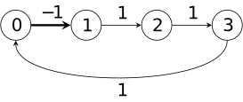
The diagram shows one horizontal row of the \(4\times 4\) torus; vertical edges are omitted. The curved edge is the periodic join. The four-step winding product is minus one, independently of the two neighboring plaquette products.
For \(L=5\), length-4 winding is absent, but each periodic row or column has straight winding walks of length 5. The changed row has 10 such based oriented walks, so \(\Delta \operatorname {tr}H^5=-20\). No other five-step return can wind: displacement 5 requires all 5 steps along that axis. The plaquette change remains \(\Delta \operatorname {tr}H^4=-32\). Consequently \[\Delta W=\frac 4{D^4}+\frac 2{D^5}+O(D^{-6}).\] Thus a period-5 hypothesis would leave an order \(D^{-5}\) term outside the claimed order \(D^{-6}\) remainder. This is why the preceding theorem requires both periods to be at least 6.
Proposition 28.5. A link current is an action derivative [fdip-0074]AGENTDRAFTED
- November 1, 2026
Proposition 28.5. A link current is an action derivative [fdip-0074]AGENTDRAFTED
- November 1, 2026
Use a complex scalar field on the unit-weight lattice of Theorem 28.2, with \(G=U(1)\), \(U_e=e^{iA_e}\) and \(m>0\). Fix an oriented edge \(e:s\to h\), and let its angle \(A_e\) vary while all other angles are fixed. For the complex matter law, write \[S_U(\phi )=\phi ^*Q_U\phi ,\qquad C_U=Q_U^{-1}.\] Define the sign of the link current by \[J_e(\phi ,U)=\frac {\partial S_U(\phi )}{\partial A_e} =2\operatorname {Im}(\overline {\phi _h}U_e\phi _s).\] Then \[\begin {aligned} \frac {\partial W}{\partial A_e} &=\operatorname {tr}_{\mathbb C} \left (C_U\frac {\partial Q_U}{\partial A_e}\right )\\ &=\mathbb E_U[J_e] =2\operatorname {Im}\bigl (U_e(C_U)_{s,h}\bigr ). \end {aligned}\] All expectations here condition on the fixed connection \(U\).
Proof.
- November 1, 2026
Proof.
- November 1, 2026
The only angle-dependent edge energy is \[|\phi _h-e^{iA_e}\phi _s|^2 =|\phi _h|^2+|\phi _s|^2 -2\operatorname {Re}(\overline {\phi _h}e^{iA_e}\phi _s).\] Its derivative is the displayed positive twice-imaginary-part expression, fixing the current sign. The matrix derivative has entries \(-iU_e\) in position \((h,s)\) and \(i\overline {U_e}\) in position \((s,h)\), and zero elsewhere. Since \(C_U\) is Hermitian, its trace pairing with that derivative is \(2\operatorname {Im}(U_e(C_U)_{s,h})\).
The determinant derivative used in the edge-variance identity applies equally to complex invertible matrices. Along this real parameter, \(Q_U\) stays positive Hermitian, so its determinant is positive and \[\frac {\partial }{\partial A_e}\log \det _{\mathbb C}Q_U =\operatorname {tr}_{\mathbb C} \left (Q_U^{-1}\frac {\partial Q_U}{\partial A_e}\right ).\] Finally, the complex Gaussian covariance gives \(\mathbb E_U[\overline {\phi _h}\phi _s]=(C_U)_{s,h}\). Substitution into the explicit current proves the expectation identity.
TauCeti's Matrix.fderiv_det_apply supplies
\(D\det (Q)[B]=\det (Q)\operatorname {tr}(Q^{-1}B)\) over a complete
nontrivially normed field when \(\det Q\) is a unit. Complex positive
definiteness supplies invertibility here. The logarithm, angle direction,
current sign and Gaussian expectation are the additional steps above;
the formal declaration does not state this current law.
For a differentiable real orthogonal family, the corresponding convention uses \(S=\frac 12\langle \phi ,Q\phi \rangle \), \(J=\partial S\) and \(W=\frac 12\log \det _{\mathbb R}Q\). Both sides then carry the same factor \(1/2\). In the complex convention used here, neither the action nor the log determinant has that factor.
29. A dynamical connection and its matter law [fdip-0075]AGENTDRAFTED
- November 2, 2026
29. A dynamical connection and its matter law [fdip-0075]AGENTDRAFTED
- November 2, 2026
The determinant action is a function of a fixed connection. A measure on connections turns that function into part of a joint law: one may first draw a connection and then draw a Gaussian matter field in it. Integrating over the matter changes the connection's probability, while conditioning on a connection recovers the background Gaussian law.
The matter determinant is at least its value on the identity connection, with equality exactly when every closed walk acts as the identity. A small square torus makes the joint law explicit. Its gauge orbits reduce the calculation to a finite sum of positive determinant weights. At zero bare gauge coupling, scalar matter already changes the plaquette expectation from zero to a strictly positive number. This finite comparison does not determine large-loop screening or an infinite-volume area law.
Definition 29.1. The joint gauge and real-matter measure [fdip-0076]AGENTDRAFTED
- November 1, 2026
Definition 29.1. The joint gauge and real-matter measure [fdip-0076]AGENTDRAFTED
- November 1, 2026
Fix the graph, positive edge weights and invariant fiber metric of a connection background. When using a Wilson action, also supply square faces and their attaching walks. Let \(G\) be a finite group, or a compact Hausdorff group supplied with a normalized bi-invariant Borel probability measure \(\mu _G\). In the finite case use uniform probability measure. Let \(\rho :G\to O(F)\) be a continuous orthogonal representation on a finite-dimensional real inner-product space; continuity is automatic for a finite group. The compact-group measure is assumed as part of the data here.
Put \(\mathcal H=F^V\), \(N=\dim _{\mathbb R}\mathcal H\) and \(d\mu (U)=\prod _{e\in E}d\mu _G(U_e)\). Choose \(m>0\) and write \(Q_U=L_U+m^2I\). Use a continuous real gauge-invariant action \(S_W(U)\), such as the Wilson action with its declared representation and coupling. With ordinary Lebesgue volume \(d\operatorname {vol}(\phi )\) in the fixed metric, define \[\begin {aligned} \mathfrak Z &=\int _{G^E}\int _{\mathcal H} e^{-S_W(U)-\frac 12\langle \phi ,Q_U\phi \rangle } \,d\operatorname {vol}(\phi )\,d\mu (U),\\ d\mathbb P(U,\phi ) &=\mathfrak Z^{-1} e^{-S_W(U)-\frac 12\langle \phi ,Q_U\phi \rangle } \,d\mu (U)\,d\operatorname {vol}(\phi ). \end {aligned}\] This is a law on both the connection and the real matter field.
The normalization is finite and positive. Indeed, \(Q_U\ge m^2I\), and the continuous action has a finite lower bound on compact \(G^E\). Thus the integrand is bounded by a constant times \(e^{-m^2\|\phi \|^2/2}\), which is integrable. It is everywhere positive. A gauge transformation preserves the edge measure by left and right invariance, the matter volume by orthogonality, and the quadratic form by gauge covariance. Hence the joint law is gauge invariant.
The edge measure differs from the unnormalized counting convention in Definition 26.3: for finite \(G\), replacing \(\mu \) by counting measure multiplies \(\mathfrak Z\) by \(|G|^{|E|}\) and leaves normalized expectations unchanged. The matter volume is also explicit: it has not been divided by \((2\pi )^{N/2}\).
Theorem 29.2. Integrating and conditioning the matter field [fdip-0077]AGENTDRAFTED
- November 1, 2026
Theorem 29.2. Integrating and conditioning the matter field [fdip-0077]AGENTDRAFTED
- November 1, 2026
For the joint law, let \(W(U)=\frac 12\log \det _{\mathbb R}Q_U\) and set \[Z_U=\int _{G^E}e^{-S_W(U)-W(U)}\,d\mu (U).\] Then \[\mathfrak Z=(2\pi )^{N/2}Z_U,\qquad d\mathbb P_U(U)=Z_U^{-1}e^{-S_W(U)-W(U)}\,d\mu (U).\] A conditional matter kernel is \[K_U(d\phi )=(2\pi )^{-N/2}(\det Q_U)^{1/2} e^{-\frac 12\langle \phi ,Q_U\phi \rangle } \,d\operatorname {vol}(\phi ),\] so, conditionally on \(U\), the field has law \(N(0,Q_U^{-1})\). In particular the induced action adds to the bare gauge action exactly, with no large-mass approximation.
Proof.
- November 1, 2026
Proof.
- November 1, 2026
The real Gaussian integral, converted from its normalized reference volume to ordinary volume, gives \[\int _{\mathcal H}e^{-\frac 12\langle \phi ,Q_U\phi \rangle } \,d\operatorname {vol}(\phi ) =(2\pi )^{N/2}e^{-W(U)}.\] Tonelli's theorem applies to the nonnegative joint density. Integrating first over \(\phi \) proves the normalization and marginal formulas. Dividing the fixed-\(U\) matter density by this Gaussian integral yields \(K_U\). Multiplying the two displayed densities recovers the joint density, proving the disintegration identity \[\mathbb P(dU,d\phi )=\mathbb P_U(dU)K_U(d\phi ).\] This explicitly chosen kernel supplies a conditional version at every connection.
Mathlib's MeasureTheory.lintegral_prod states Tonelli's
identity for an almost-everywhere measurable nonnegative extended-real
function, with an s-finite inner measure. The gauge probability and
finite-dimensional Lebesgue measure satisfy these measure conditions;
the density here is measurable. This is partial support for the
product-integration step, not for the Gaussian evaluation or the
marginal and conditional formulas derived above.
The selected Gaussian marginal and conditional propagator formulas therefore apply separately at each fixed \(U\). For example, in orthonormal retained and eliminated coordinates, write \[Q_U=\begin {pmatrix}A_U&B_U\\B_U^T&C_U\end {pmatrix},\qquad C_U>0.\] Then the retained precision at that connection is \(A_U-B_UC_U^{-1}B_U^T\), and \[\phi _{\mathrm {elim}}\mid (\phi _{\mathrm {ret}}=x,U) \sim N(-C_U^{-1}B_U^Tx,C_U^{-1}).\] These statements keep the connection in the conditioning data.
After averaging over \(U\), the matter law is generally a mixture of Gaussian laws, rather than one Gaussian law. Its covariance is \[\mathbb E_{\mathbb P_U}[Q_U^{-1}],\] by the conditional covariance identity and the zero conditional mean. Observing retained matter coordinates also reweights the distribution of \(U\) by their conditional likelihood. One cannot obtain the joint conditional law by keeping the original connection probabilities fixed and applying a single Gaussian formula.
Theorem 29.3. The matter determinant is smallest on the identity orbit [fdip-00A6]AGENTDRAFTED
- November 2, 2026
Theorem 29.3. The matter determinant is smallest on the identity orbit [fdip-00A6]AGENTDRAFTED
- November 2, 2026
The massive precision \(Q_U\) depends on the connection. Gauge covariance makes its determinant constant on orbits. The comparison below identifies the minimum. It is the value on the identity connection, attained exactly when every closed walk acts as the identity on the fiber.
Let \(F\) have dimension \(n\) over its scalar field, and let \(Q_1\) be the scalar massive precision of the same finite graph, the same positive edge weights, and the same mass \(m>0\). For every connection, \(\det Q_U\ge (\det Q_1)^n\). Equality holds if and only if every closed walk acts as the identity on \(F\). Every connection in the identity orbit has that property. So does every connection whose holonomy acts through the kernel of \(\rho \).
Proof.
- November 2, 2026
Proof.
- November 2, 2026
Write \(D\) for the positive diagonal operator on scalar functions with \(D_v=m^2+\sum _{e\ni v}w_e\), and write \(D_H\) for \(D\) acting separately on each fiber. The quadratic form in the connection background expands as \(\langle f,Q_Uf\rangle =\sum _v D_v\|f_v\|^2-\sum _e 2w_e\operatorname {Re}\langle f(h(e)),U_ef(s(e))\rangle \). The associated self-adjoint operator is \(Q_U=D_H-H_U\), where the only nonzero blocks of \(H_U\) are \(w_eU_e\) and \(w_eU_e^*\). Let \(K_U=D_H^{-1/2}H_UD_H^{-1/2}\). Then \(Q_U=D_H^{1/2}(I-K_U)D_H^{1/2}\), so \(\det Q_U=(\det D)^n\det (I-K_U)\). The identity connection has \(Q_I=Q_1\otimes I_F\), hence \((\det Q_1)^n=\det Q_I\). It is enough to compare \(I-K_U\) with \(I-K_I\).
The scalar adjacency \(A\) has the same off-diagonal weights. Its normalized operator \(K_1=D^{-1/2}AD^{-1/2}\) is self-adjoint, and \(K_I=K_1\otimes I_F\). The similar operator \(D^{-1}A\) has row sums \(\bigl (\sum _{e\ni v}w_e\bigr )/D_v<1\), because \(m>0\). The maximum absolute row sum is strictly less than \(1\), so the spectral radius of \(D^{-1}A\) is strictly less than \(1\). Since \(K_1=D^{1/2}(D^{-1}A)D^{-1/2}\), the operator \(K_1\) has the same spectral radius. Self-adjointness gives \(\|K_1\|=\rho (K_1)<1\).
The same comparison bounds the connection. For a section \(f\), set \(y_v=\|f_v\|\). Each fiber of \(H_U\) has operator norm \(w_e\), so \(\|(H_Uf)_v\|\le (Ay)_v\). Conjugating by \(D^{1/2}\) yields \(\|(K_Uf)_v\|\le (K_1y)_v\). Therefore \(\|K_Uf\|\le \|K_1y\|\le \|K_1\|\|f\|\), and \(\|K_U\|<1\). The eigenvalues of the self-adjoint operator \(K_U\) are real and lie in the open interval \((-1,1)\).
For every such eigenvalue, \(\log (1-\lambda )=-\sum _{k\ge 1}\lambda ^k/k\). Summing over eigenvalues gives \(\log \det (I-K_U)=-\sum _{k\ge 1}\frac 1k\operatorname {tr}(K_U^k)\). Expanding the trace in walks, a closed walk \(\gamma \) of length \(k\) contributes its positive weight \(w(\gamma )=\prod _{e\in \gamma }\frac {w_e}{\sqrt {D_{s(e)}D_{h(e)}}}\) times the trace of its holonomy. The holonomy is the ordered product of the fiber maps, with the first edge on the right, because parallel transport along \(e\) sends \(f(s(e))\) to \(U_ef(s(e))\). A unitary or orthogonal map has eigenvalues on the circle, so the real part of its trace is at most \(n\), with equality exactly when the map is the identity. The trace \(\operatorname {tr}(K_U^k)\) is real and equals the sum of those real parts against the walk weights. Hence \(\operatorname {tr}(K_U^k)\le \operatorname {tr}(K_I^k)=n\operatorname {tr}(K_1^k)\). Since each trace is at most the corresponding identity trace, \(\log \det (I-K_U)\ge \log \det (I-K_I)\). The logarithm is increasing, and \(\det (I-K_U)\ge \det (I-K_I)\). The powers of \(\det D\) cancel in the comparison. This is the asserted lower bound.
Equality of the determinants forces equality of the two series. For every \(k\ge 1\), \[\operatorname {tr}(K_U^k)=\operatorname {tr}(K_I^k).\] Their difference is the sum, over closed walks, of the positive weight times \(n-\operatorname {Re}\operatorname {tr}\operatorname {Hol}(\gamma )\). Each summand is nonnegative, so each vanishes. Every closed walk therefore acts as the identity on \(F\). Conversely, that condition makes every walk contribution agree with the identity connection, and the determinants agree.
These connections are exactly the identity orbit in the represented gauge group. Choose a root in each connected component and propagate \(\rho (U)\) along any walk from that root. The product is independent of the walk because every closed walk acts as the identity. The resulting vertex operators \(g_v\) satisfy \(U_e=g_{h(e)}g_{s(e)}^{-1}\). In the other direction, a gauge transform of the identity has determinant \(\det Q_I\) by the covariance already cited. A holonomy in the kernel of \(\rho \) is invisible to \(Q_U\): equality sees the action on \(F\), not a finer group element.
When \(F\) is real, the induced action \(W(U)=\frac 12\log \det Q_U\) of the joint law is therefore smallest exactly on this orbit. When \(F\) is complex, the same bound says that \((\det Q_U)^{-1}\) is largest there. The massless operator is outside the argument: its identity connection can be singular, and a nontrivial represented holonomy can leave a parallel section, so a zero determinant does not characterize the identity orbit.
On the three-by-three torus with unit weights and mass squared equal to \(1\), the all-positive connection lies on the identity orbit and attains the bound. The torus sum records that determinant.
Example 29.4. An exact matter-weighted sum on the three-by-three torus [fdip-0078]AGENTDRAFTED
- November 2, 2026
Example 29.4. An exact matter-weighted sum on the three-by-three torus [fdip-0078]AGENTDRAFTED
- November 2, 2026
On a connected graph, take \(G=\{1,-1\}\) acting by multiplication on the real line. Two gauges induce the same action precisely when their ratio is constant, so each orbit contains \(2^{|V|-1}\) connections. A spanning tree meets every vertex and contains no cycle. Requiring its edges to be positive selects one connection from each orbit. With \(b_1=|E|-|V|+1\) and with zero bare coupling, gauge invariance of the determinant converts the marginal into \[Z_U=2^{-b_1}\sum _s(\det Q_s)^{-1/2},\] where \(s\) runs through the sign patterns on the complementary edges.
Take the square torus with both periods three, \(G=\{1,-1\}\), real scalar matter, unit edge weights, \(m^2=1\) and bare coupling \(\beta =0\). Vertices are \((x,y)\) with coordinates in \(\mathbb Z/3\mathbb Z\); use horizontal edges \(a_{x,y}\) and vertical edges \(b_{x,y}\) in the orientations of that definition. There are 9 matter coordinates and 18 links.
Fix a spanning tree by requiring \[a_{0,y}=a_{1,y}=1\quad (y=0,1,2),\qquad b_{0,0}=b_{0,1}=1.\] These 8 edges connect every vertex without a cycle. Parameterize the 10 remaining links by \(s=(s_1,\ldots ,s_{10})\in \{1,-1\}^{10}\): \[\begin {aligned} (a_{2,0},a_{2,1},a_{2,2})&=(s_1,s_2,s_3),\\ (b_{1,0},b_{2,0},b_{1,1},b_{2,1})&=(s_4,s_5,s_6,s_7),\\ (b_{0,2},b_{1,2},b_{2,2})&=(s_8,s_9,s_{10}). \end {aligned}\] Let \(U_e(s)\) denote these assigned signs.
In the vertex order \((0,0),(1,0),(2,0),(0,1),\ldots ,(2,2)\), let \(E_{v,w}\) be a matrix unit and define \[\begin {aligned} H_s&=\sum _{e\in E}U_e(s)(E_{h(e),s(e)}+E_{s(e),h(e)}),\\ d_s&=\det (5I-H_s),\\ P_{x,y}(s)&=a_{x,y}b_{x+1,y}a_{x,y+1}b_{x,y},\\ k(s)&=\#\{(x,y):P_{x,y}(s)=-1\}. \end {aligned}\] The symbol \(s(e)\) in a matrix index is the edge's source vertex; the tuple \(s\) labels the 10 free signs. All subscripts on links are read modulo three. Every \(d_s\) is a positive integer.
For each connection there is a unique gauge transformation with value one at \((0,0)\) that makes the tree links positive: propagate its vertex values along the tree. The only remaining transformations fixing a connection are the two constant signs, since the graph is connected. Hence every gauge orbit has \(2^8\) elements and exactly one displayed representative. Gauge-invariant normalized edge sums therefore reduce to the following exact formulas: \[\begin {aligned} R&=\sum _{s\in \{1,-1\}^{10}}d_s^{-1/2},& Z_U&=2^{-10}R,\\ \langle P_{0,0}\rangle &=\frac {\sum _sP_{0,0}(s)d_s^{-1/2}}{R},& \mathfrak Z&=(2\pi )^{9/2}Z_U. \end {aligned}\] Here \(Z_U\) is the determinant-weighted edge integral, whereas \(\mathfrak Z\) includes ordinary matter volume.
The finite sums contain 1024 terms. They can be evaluated by forming the displayed integer matrix for each sign tuple and taking its determinant. At the all-positive tuple, the eigenvalues of \(5I-H_s\) are \(1\), 4 copies of \(4\), and 4 copies of \(7\), so \(d_s=4^4\cdot 7^4=614656\). This is the lower bound of the matter-determinant comparison. Grouping by the number of negative plaquettes gives the table. The matter probability in row \(k\) is \(R^{-1}\sum _{s:k(s)=k}d_s^{-1/2}\), and the probability without matter is the orbit count divided by \(1024\).
\[\begin {array}{c|r|c|c} k&\text {orbits}&\text {pure gauge }(\beta =0)&\text {with matter}\\\hline 0&4&0.00390625&0.00404317\\ 2&144&0.14062500&0.14286686\\ 4&504&0.49218750&0.49338270\\ 6&336&0.32812500&0.32522204\\ 8&36&0.03515625&0.03448524 \end {array}\]Translation invariance gives the same expectation at every plaquette. The pure-gauge torus law at \(\beta =0\) instead has \(\langle P_{0,0}\rangle =0\). No large-mass truncation was used in these finite sums.
Proposition 29.5. A finite loop comparison does not determine screening [fdip-0079]AGENTDRAFTED
- November 1, 2026
Proposition 29.5. A finite loop comparison does not determine screening [fdip-0079]AGENTDRAFTED
- November 1, 2026
On a square torus of periods at least three, use the joint law with \(G=\{1,-1\}\) acting by multiplication on the real field \(\phi \in \mathbb R^V\), unit weights, \(m>0\) and \(\beta =0\). For any simple nonempty closed edge cycle \(C\), its Wilson product \(W_C(U)=\prod _{e\in C}U_e\) has \[\langle W_C\rangle _{\mathrm {matter}}>0,\qquad \langle W_C\rangle _{\mathrm {pure}}=0.\] In particular, the strict positivity in the three-by-three example has a direct proof independent of rounding the determinant sums.
Proof.
- November 1, 2026
Proof.
- November 1, 2026
Put \(D=4+m^2\). For the real scalar convention, the joint Boltzmann factor at zero bare gauge coupling is \[\exp \left (-\frac D2\sum _v\phi _v^2\right ) \prod _{e\in E}\exp (U_e\phi _{s(e)}\phi _{h(e)}).\] Average the independent edge signs before integrating the matter. Since \[\frac 12\sum _{u=\pm 1}e^{ut}=\cosh t,\qquad \frac 12\sum _{u=\pm 1}u e^{ut}=\sinh t,\] the Wilson expectation is \(I_C/I_{\varnothing }\), where \[\begin {aligned} I_C={}&\int _{\mathbb R^V}e^{-\frac D2\sum _v\phi _v^2} \prod _{e\in C}\sinh (\phi _{s(e)}\phi _{h(e)})\\ &\qquad \qquad \cdot \prod _{e\notin C} \cosh (\phi _{s(e)}\phi _{h(e)})\,d\phi . \end {aligned}\] For \(C=\varnothing \), every edge contributes a hyperbolic cosine. For nonzero vertex coordinates, the sign of the numerator's product of hyperbolic sines is \[\prod _{e\in C}\operatorname {sgn}(\phi _{s(e)}\phi _{h(e)}) =\prod _{v\in C}\operatorname {sgn}(\phi _v)^2=1.\] Each cycle vertex occurs twice. All other factors are strictly positive, so the numerator integrand is positive off coordinate hyperplanes. Its absolute value is bounded by the denominator integrand because \(|\sinh t|\le \cosh t\). Positive mass makes the latter integrable by the joint-law bound. Both integrals are therefore finite and strictly positive. In the pure law, independent uniform edge signs give zero expectation for any nonempty product of distinct edges, proving the comparison.
Integrating matter has changed the connection law, so the exact pure-gauge formula cannot be reused unchanged. On tori with periods at least 6, the closed-walk calculation gives a separate controlled large-mass explanation: matter generates a positive plaquette coefficient and higher loop terms. Its order \(D^{-6}\) remainder is not being applied to the three-by-three example, where short winding cycles occur.
Neither the finite comparison nor the positive plaquette term establishes an asymptotic area law, a perimeter law or string breaking. Such a claim needs a specified family of volumes and loops, a limiting regime and control of the higher terms. Gliozzi and Rago study a different system: a three-dimensional two-element gauge group coupled to Ising matter taking only the values \(\pm 1\), rather than an unbounded Gaussian field. Their Section 3, equation (12), fixes that action; their analysis of Wilson-loop overlap with a broken-string state is model-specific context [gliozzi2004overlap, pp. 2, 5]. It does not supply a screening theorem for the present Gaussian law.
30. Compact gauge groups and representation data [fdip-007A]AGENTDRAFTED
- November 1, 2026
30. Compact gauge groups and representation data [fdip-007A]AGENTDRAFTED
- November 1, 2026
Replacing a finite gauge group by a compact group changes edge sums into normalized Haar integrals. Character orthogonality survives, but an infinite character expansion needs a convergence argument before it can be inserted into a surface partition function. The distinction between an \(L^2\) expansion and an absolutely convergent kernel is therefore part of the model.
For the circle group, Wilson and Villain weights give explicit Fourier coefficients. Matching one coefficient does not match the whole law. For matrix groups, a separate smooth-field calculation explains the classical small-spacing normalization of the Wilson action. Neither calculation constructs a quantum continuum limit.
Unit quaternions identify the compact group \(SU(2)\) and its binary polyhedral subgroups. A representation datum then specifies which group acts on which field and whether it also moves the substrate. These choices precede any physical comparison.
Theorem 30.1. Normalized Haar measure [fdip-007B]AGENTDRAFTED
- November 1, 2026
Theorem 30.1. Normalized Haar measure [fdip-007B]AGENTDRAFTED
- November 1, 2026
Every compact Hausdorff topological group \(G\) has a unique regular Borel probability measure \(\mu _G\) invariant under left translation. This is the normalized Haar theorem, used here as a cited statement; existence and uniqueness are not proved in these notes. The existence and uniqueness-up-to-scale statements are Theorems 4.3 and 4.6 in [gleason2010haar, pp. 6, 11]. Compactness permits normalization to total mass one.
The normalized measure is also invariant under right translation and inversion. Indeed, a right translate of \(\mu _G\) is another left-invariant regular probability measure, hence equals \(\mu _G\) by uniqueness. The pushforward under inversion is then left invariant, because inversion changes left translations into right translations; it too has total mass one and equals \(\mu _G\). These deductions explain why the same measure works with either orientation of an edge.
Every nonempty open set has positive Haar measure. If an open set had measure zero, choose a point in it; its left translates cover \(G\), and compactness gives a finite subcover, contradicting total mass one. Consequently a continuous function that vanishes \(\mu _G\)-almost everywhere vanishes everywhere.
For a finite group this measure is uniform counting. For \(U(1)=\{e^{i\theta }:\theta \in \mathbb R\}\), it is \(d\theta /(2\pi )\) on one period: translation invariance and total mass one identify this measure by uniqueness. Product Haar measure on the edge space \(G^E\) supplies the compact measure assumed in the joint matter law. For \(U(1)\) and \(SU(2)\), all spaces here are compact metrizable, so their Borel products have the usual product measurable structure.
Mathlib constructs Haar measure as
MeasureTheory.Measure.haarMeasure, normalized on a chosen
compact set with nonempty interior; for compact \(G\), choose that
set to be all of \(G\). The separate declaration
MeasureTheory.Measure.isHaarMeasure_eq_of_isProbabilityMeasure
asserts equality of two Haar probability measures on a locally compact
topological group with its Borel measurable structure. It has no
second-countability assumption. These are correspondences for the
construction and normalized uniqueness, respectively; the right and
inversion invariance arguments above are stated separately.
Theorem 30.2. Compact character expansions and surface integrals [fdip-007C]AGENTDRAFTED
- November 1, 2026
Theorem 30.2. Compact character expansions and surface integrals [fdip-007C]AGENTDRAFTED
- November 1, 2026
Let \(G\) be a compact Lie group with normalized Haar measure. Choose unitary representatives of its complex irreducibles, indexed by \(\widehat G\), with dimensions \(d_\rho \). The Peter–Weyl theorem says that the functions \(\sqrt {d_\rho }\rho (\cdot )_{ij}\) form an orthonormal basis of \(L^2(G)\). Its central subspace has orthonormal basis \(\chi _\rho \). Thus a central \(f\in L^2(G)\) has the expansion \[f=\sum _{\rho \in \widehat G}c_\rho \chi _\rho , \qquad c_\rho =\int _G f(h)\overline {\chi _\rho (h)}\,d\mu _G(h),\] with convergence in \(L^2\). This is a cited statement, namely Woit's Section 5, Theorem 1 and Corollary 1 [woit2012peterweyl, p. 6]. It does not assert pointwise or absolute convergence for an arbitrary \(L^2\) function.
For an inequivalent exhaustive family of finite-dimensional unitary
continuous models, TauCeti's
TauCeti.peterWeylBasis constructs the normalized
matrix-coefficient Hilbert basis, with its inner-product convention
for matrix coefficients. Over \(\mathbb C\), its coefficient
\(\langle \rho (g)e_a,e_b\rangle \) is the conjugate of the matrix
entry \(\rho (g)_{ba}\); conjugation, or reindexing by dual
representations, gives the equivalent entry-coordinate basis.
The separate TauCeti.characterBasis constructs
the actual character basis of the central \(L^2\) subspace.
Compact Hausdorff groups over \(\mathbb C\), hence the compact Lie
groups here, satisfy the stated hypotheses. These correspondences
support the two \(L^2\) basis statements, not the uniform absolute
convergence or surface integral established next.
Suppose now that \(f\) is continuous and central and that \[\sum _{\rho \in \widehat G}|c_\rho |d_\rho <\infty .\] Then its character expansion converges uniformly and absolutely. For the closed oriented polygonal surface, with \(P\) faces and genus \(g\), define the edge integral \[Z_\Sigma (f)=\int _{G^E}\prod _p f(U_p)\,d\mu (U).\] Under the displayed summability condition, \[Z_\Sigma (f)=\sum _{\rho \in \widehat G} d_\rho ^{2-2g}\left (\frac {c_\rho }{d_\rho }\right )^P,\] and this numerical series is absolutely convergent.
Proof.
- November 1, 2026
Proof.
- November 1, 2026
Unitarity gives \(|\chi _\rho (h)|\le d_\rho \). The sum of the uniform bounds is finite, so the character series has a continuous uniform limit. Peter–Weyl identifies that limit with \(f\) in \(L^2\); continuity and full support of Haar measure make the equality pointwise. Expanding a product over the finite face set gives a sum whose total absolute value is bounded uniformly by \[\left (\sum _\rho |c_\rho |d_\rho \right )^P.\] This bound is integrable against probability measure, justifying interchange of the full face-label sum and the edge integrals.
Haar averaging gives the same matrix orthogonality as finite averaging: for \(A:V_\tau \to V_\rho \), the integral \(\int _G\rho (h)A\tau (h)^{-1}\,d\mu _G(h)\) is an intertwiner. Schur's lemma and its trace make it zero for inequivalent representatives and \((\operatorname {tr}A/d_\rho )I\) for equal ones. The edge contractions and circular vertex links in the finite surface proof therefore leave one common face label and one free index per vertex. Their contribution is \(c_\rho ^P d_\rho ^{|V|-|E|}\), the displayed formula. Absolute convergence follows as well: the absolute values of these integrated terms are bounded by the integrals of the absolute face terms, whose total has just been bounded. In particular \(f=1\) still gives \(Z_\Sigma (1)=1\).
Definition 30.3. Convolution kernels with positive coefficients [fdip-007I]AGENTDRAFTED
- November 1, 2026
Definition 30.3. Convolution kernels with positive coefficients [fdip-007I]AGENTDRAFTED
- November 1, 2026
For a finite or compact Lie group \(G\), use the normalized Haar measure, irreducibles and dimensions of the character expansion. For convolution constructions, consider real continuous central kernels \(k\) with the separate hypotheses \[\begin {gathered} k(h)>0,\qquad k(h^{-1})=k(h),\\ k(h)=\sum _{\rho \in \widehat G}d_\rho a_\rho \chi _\rho (h), \qquad a_\rho >0,\qquad \sum _{\rho \in \widehat G}d_\rho ^2a_\rho <\infty . \end {gathered}\] The last condition gives uniform absolute convergence; inversion symmetry and reality impose the corresponding agreement of conjugate coefficients. The convention is \(c_\rho =d_\rho a_\rho \), not \(c_\rho =a_\rho \). These are assumptions on a kernel, not consequences of the Peter–Weyl theorem. In particular, pointwise positivity does not imply the coefficient condition, as the circle counterexample shows.
Example 30.4. A positive weight with a negative coefficient [fdip-007J]AGENTDRAFTED
- November 1, 2026
Example 30.4. A positive weight with a negative coefficient [fdip-007J]AGENTDRAFTED
- November 1, 2026
On \(U(1)\), take \(0<\epsilon <1\) and \[k(e^{i\theta })=1-\epsilon \cos \theta =1-\frac \epsilon 2 e^{i\theta }-\frac \epsilon 2 e^{-i\theta }.\] This is a real continuous central function, unchanged by inversion, and \(k\ge 1-\epsilon >0\). Its character coefficients at \(n=\pm 1\) are nevertheless \(-\epsilon /2\). Thus the pointwise and Fourier positivity assumptions in the kernel definition are distinct.
Proposition 30.5. Wilson and Villain coefficients on the circle [fdip-007D]AGENTDRAFTED
- November 1, 2026
Proposition 30.5. Wilson and Villain coefficients on the circle [fdip-007D]AGENTDRAFTED
- November 1, 2026
For \(G=U(1)\), use characters \(\chi _n(e^{i\theta })=e^{in\theta }\) with \(n\in \mathbb Z\) and normalized Haar measure \(d\theta /(2\pi )\). For \(\beta >0\), the Wilson weight \(w_\beta (\theta )=e^{\beta \cos \theta }\) has coefficients \[I_n(\beta )=\sum _{j=0}^\infty \frac {(\beta /2)^{2j+|n|}}{j!(j+|n|)!}>0, \qquad \sum _{n\in \mathbb Z}I_n(\beta )=e^\beta .\] Thus its character series is uniformly absolutely convergent. The Wilson action convention includes the additional constant factor \(e^{-\beta }\); this multiplies all coefficients but cancels from the normalized one-plaquette probability.
TauCeti's
Real.integral_exp_mul_cos_mul_cexp
proves the Wilson circle integral with exponent \(+in\theta \) and
unnormalized measure on \([-\pi ,\pi ]\). Replacing \(n\) by \(-n\)
and dividing by \(2\pi \) gives the coefficient convention here;
its Bessel value has the displayed power series. This correspondence
supports the Wilson coefficient identity, not the Villain formula
or the comparison of the two weights.
For \(\beta _V>0\), the Villain weight is the periodic Gaussian \[v_{\beta _V}(\theta )=\sum _{\ell \in \mathbb Z} \exp \left [-\frac {\beta _V}{2}(\theta -2\pi \ell )^2\right ].\] Its character coefficient is \[c_n^V=(2\pi \beta _V)^{-1/2} e^{-n^2/(2\beta _V)}.\] The coefficient series is again uniformly absolutely convergent and all coefficients are strictly positive. Dividing each weight by its zeroth coefficient normalizes its integral to one, giving \[\widehat c_n^W=\frac {I_n(\beta )}{I_0(\beta )},\qquad \widehat c_n^V=e^{-n^2/(2\beta _V)}.\] These normalized coefficients differ from the unnormalized \(c_\rho \) in the surface formula.
Proof.
- November 1, 2026
Proof.
- November 1, 2026
Put \(z=e^{i\theta }\). Multiply the two absolutely convergent series for \(\exp (\beta z/2)\) and \(\exp (\beta z^{-1}/2)\). The coefficient of \(z^n\) is the displayed \(I_n\); the total of all absolute coefficients is the product \(e^{\beta /2}e^{\beta /2}\). Every \(I_n\) is positive for \(\beta >0\).
For the periodic Gaussian, uniform Gaussian tail bounds on a period justify continuity and integration term by term. Unfolding its coefficient integral gives \[c_n^V=\frac 1{2\pi }\int _{\mathbb R} e^{-\beta _V x^2/2}e^{-inx}\,dx.\] For real \(t\), let \(J(t)\) be the integral without \(1/(2\pi )\) and with \(n\) replaced by \(t\). Gaussian domination permits differentiation under the integral. Integration by parts, with vanishing boundary terms, gives \(J'(t)=-(t/\beta _V)J(t)\). Since \(J(0)=\sqrt {2\pi /\beta _V}\), this proves the coefficient formula. The Gaussian coefficient bound is summable over \(n\). Its uniformly convergent Fourier series has the same coefficients as the continuous periodic Gaussian, so completeness of the character basis and continuity identify the two functions. Finally, the integral of a weight is its zeroth coefficient, which proves the normalization.
Both positive-parameter weights satisfy the positive-character kernel hypotheses: they are real, strictly positive, invariant under inversion, and have positive summable coefficients. For \(U(1)\) every irreducible dimension is one. This checks the kernel assumptions without asserting any transfer-operator or continuum conclusion.
Theorem 30.6. The matched Wilson and Villain laws differ [fdip-007E]AGENTDRAFTED
- November 2, 2026
Theorem 30.6. The matched Wilson and Villain laws differ [fdip-007E]AGENTDRAFTED
- November 2, 2026
A single \(U(1)\) plaquette has the normalized Wilson or Villain weight. Matching their fundamental Fourier coefficients determines a Villain coupling for every Wilson coupling. The two probability laws still differ.
For \(\beta >0\), write \(r(\beta )=I_1(\beta )/I_0(\beta )\) and \(\beta _V(\beta )=-\frac {1}{2\log r(\beta )}\). Then \(0<r(\beta )<1\), the matched Villain coefficient is \(r(\beta )^{n^2}\), and \[\frac {\widehat c_n^W}{\widehat c_n^V}\to \infty \] as \(|n|\to \infty \). In particular the two normalized weights are distinct, so they define distinct probability laws on the circle. The second Wilson coefficient is \(1-\frac {2r(\beta )}{\beta }\).
Proof.
- November 2, 2026
Proof.
- November 2, 2026
The series for \(I_1\) has positive terms, so \(r>0\). With normalized Haar measure, \[\int (1-\cos \theta )\,e^{\beta \cos \theta }\,\frac {d\theta }{2\pi } =I_0(\beta )-I_1(\beta ).\] The integrand is nonnegative and not identically zero, and the exponential is positive, so the integral is positive. Thus \(r<1\), the logarithm is negative, and \(\beta _V\) is positive. The Villain normalization in the coefficient note gives \(\widehat c_n^V=\exp (-n^2/(2\beta _V))\). Substituting the displayed \(\beta _V\) produces \(1/(2\beta _V)=-\log r\), hence \(\widehat c_n^V=r^{n^2}\).
The \(j=0\) term of the series for \(I_n(\beta )\), with \(n\ge 0\), is \((\beta/2)^n/n!\). Every term is positive, so \(I_n(\beta )\ge (\beta/2)^n/n!\). Therefore \(\widehat c_n^W=I_n(\beta )/I_0(\beta )\) satisfies \[\frac {\widehat c_n^W}{r^{n^2}} \ge \frac {(\beta/2)^n}{n!\,I_0(\beta )\,r^{n^2}}.\] For \(n\ge 1\), one has \(n!\le n^n\), so the logarithm of the right-hand side is at least \(n\log (\beta/2)-n\log n-\log I_0(\beta )-n^2\log r\). The last summand tends to \(+\infty \) because \(\log r<0\), and it dominates the remaining terms. The lower bound tends to infinity, and so does the ratio, as \(n\to +\infty \). The series in the coefficient note depends on \(|n|\), so \(I_n(\beta )=I_{-n}(\beta )\). The matched Villain coefficient \(r^{n^2}\) is likewise unchanged when \(n\) is replaced by \(-n\). The ratio at \(-n\) equals the ratio at \(n\), and the same limit holds as \(|n|\to \infty \).
The coefficient note identifies each normalized continuous weight with its Fourier series. Some coefficient of large order differs, so the weights differ as functions and as probability laws.
The same series gives the second coefficient. The identity \(\frac {2}{\beta }(\beta/2)^{2j+1}=(\beta/2)^{2j}\) rewrites \[\frac {2}{\beta }I_1(\beta ) =\sum _{j\ge 0}\frac {(\beta/2)^{2j}}{j!\,(j+1)!}.\] Subtracting from \(I_0\) cancels the \(j=0\) term. For \(j\ge 1\) the difference of the summands is \(\frac {(\beta/2)^{2j}\,j}{j!\,(j+1)!} =\frac {(\beta/2)^{2j}}{(j-1)!(j+1)!}\), which is the \(j-1\) term of \(I_2\). Hence \(I_0-I_2=\frac {2}{\beta }I_1\), and \(\widehat c_2^W=1-\frac {2r(\beta )}{\beta }\). At \(\beta =2\) this coefficient is \(1-r(2)\), while the matched Villain coefficient is \(r(2)^4\).
The comparison is a one-plaquette identity. It does not assert a many-plaquette continuum limit.
Proposition 30.7. The classical small-spacing Wilson action [fdip-007F]AGENTDRAFTED
- November 1, 2026
Proposition 30.7. The classical small-spacing Wilson action [fdip-007F]AGENTDRAFTED
- November 1, 2026
Fix a flat \(d\)-dimensional torus with \(d\ge 2\), a compact Lie group \(G\), and a unitary representation \(\rho :G\to U(r)\), \(r>0\). Choose smooth periodic Hermitian fields \(A_j(x)\) such that \(iA_j(x)\) lies in the image of the derived Lie-algebra representation. All derivative bounds are fixed as the mesh spacing \(a\to 0\); take meshes whose periods fit the torus. Define head-directed midpoint links \[U_j(x)=\exp \left (ia A_j(x+\tfrac a2 e_j)\right ).\] With the rightmost-first transport convention, the \(j\)-then-\(k\) plaquette is \[U_{jk}(x)=U_k(x)^*U_j(x+ae_k)^*U_k(x+ae_j)U_j(x).\] Its curvature convention is \[F_{jk}=\partial _jA_k-\partial _kA_j-i[A_j,A_k].\] The matrices \(F_{jk}\) are Hermitian.
For the Wilson action \[S_W(a)=\beta \sum _x\sum _{j<k} \left (1-\frac {\operatorname {Re}\operatorname {tr}U_{jk}(x)}r\right ),\] one has \[S_W(a)=\frac {\beta a^{4-d}}{2r} \int \sum _{j<k}\operatorname {tr}(F_{jk}(x)^2)\,dx +O(\beta a^{5-d}).\] This is a statement about evaluating a discrete action on a fixed smooth field. The constant in the remainder depends on that field, the fixed torus and the representation.
Proof.
- November 1, 2026
Proof.
- November 1, 2026
Taylor-expand the 4 midpoint values at \(x\) and use \(e^{iaA}=I+iaA-\tfrac 12a^2A^2+O(a^3)\). The terms of order \(a\) cancel. The variation of the two transverse links contributes \(ia^2(\partial _jA_k-\partial _kA_j)\); the products of first-order terms contribute \(a^2[A_j,A_k]\). The midpoint derivatives along each link cancel between opposite traversals. Hence, uniformly in \(x\), \[U_{jk}(x)=I+ia^2F_{jk}(x)+O(a^3).\] To obtain the real trace to the needed order, use the exact identity for a unitary \(r\times r\) matrix: \[1-\frac {\operatorname {Re}\operatorname {tr}U}{r} =\frac 1{2r}\operatorname {tr}\bigl ((U-I)^*(U-I)\bigr ).\] Substitution yields \[1-\frac {\operatorname {Re}\operatorname {tr}U_{jk}(x)}r =\frac {a^4}{2r}\operatorname {tr}(F_{jk}(x)^2)+O(a^5).\] There are \(O(a^{-d})\) plaquettes. After multiplication by \(a^d\), the Riemann sum for \(\sum _{j<k}\operatorname {tr}(F_{jk}^2)\) differs from its integral by \(O(a)\). Summing the uniform error and this Riemann-sum error proves the formula.
To fix a component convention, suppose the Hermitian generators in the chosen representation satisfy \[\operatorname {tr}(T_\alpha T_\gamma ) =T(\rho )\delta _{\alpha \gamma },\qquad T(\rho )>0.\] Write \(F_{jk}=\sum _\alpha F_{jk}^\alpha T_\alpha \) and fix \(g>0\). Choosing \[\beta =\frac {r a^{d-4}}{T(\rho )g^2}\] gives the classical limit \[\begin {aligned} S_W(a)&=\frac 1{2g^2}\int \sum _{j<k,\alpha }(F_{jk}^\alpha )^2\,dx+O(a)\\ &=\frac 1{4g^2}\int \sum _{j,k,\alpha }(F_{jk}^\alpha )^2\,dx+O(a). \end {aligned}\] The second sum counts both orders, with \(F_{kj}=-F_{jk}\) and \(F_{jj}=0\). The trace normalization is an explicit assumption; it must not be imposed on directions annihilated by a nonfaithful representation. For the fundamental representation of \(SU(r)\) with \(T(\rho )=1/2\), this is \(\beta =2r a^{d-4}/g^2\). For unit-charge \(U(1)\), \(r=T(\rho )=1\), giving \(\beta =a^{d-4}/g^2\).
The matrices \(A_j\) are those appearing in the link exponential; any coupling absorbed into them must be retained when comparing component conventions. Wingate's equation (6.20) and Exercise 2 [wingate2025lattice, p. 8] give the Wilson-action context and the four-dimensional fundamental normalization. The ordered expansion and error estimate above are derived with the convention stated here. They do not prove convergence of lattice probability measures, renormalization or the existence of a quantum continuum theory.
Proposition 30.8. Unit quaternions and binary rotation groups [fdip-007G]AGENTDRAFTED
- November 1, 2026
Proposition 30.8. Unit quaternions and binary rotation groups [fdip-007G]AGENTDRAFTED
- November 1, 2026
The unit quaternions are isomorphic to \(SU(2)\) by \[M(a+bi+cj+dk)= \begin {pmatrix}a+bi&c+di\\-c+di&a-bi\end {pmatrix}.\] Conjugation on the imaginary quaternions defines a surjective homomorphism \[\pi :SU(2)\longrightarrow SO(3),\qquad \pi (M(q))(v)=qvq^{-1},\qquad \ker \pi =\{1,-1\}.\] For the proper rotation groups \(R_T,R_O,R_I\) of the regular tetrahedron, octahedron and icosahedron, define \[2T=\pi ^{-1}(R_T),\qquad 2O=\pi ^{-1}(R_O),\qquad 2I=\pi ^{-1}(R_I).\] Their orders are respectively \(24,48,120\). Each quotient by \(\{1,-1\}\) is its indicated rotation group.
Proof.
- November 1, 2026
Proof.
- November 1, 2026
The images of \(i,j,k\) satisfy the quaternion multiplication relations, so \(M\) is an injective real-algebra homomorphism. Direct calculation gives \[M(q)^*M(q)=|q|^2I,\qquad \det M(q)=|q|^2.\] Conversely, a special unitary matrix of degree two has the form \[\begin {pmatrix}z&w\\-\overline w&\overline z\end {pmatrix}, \qquad |z|^2+|w|^2=1,\] by orthonormality of its columns and determinant one. Taking real and imaginary parts of \(z,w\) gives a unique unit quaternion. This proves the group identification.
Conjugation preserves imaginary quaternions and their norm, so gives an orthogonal map of \(\mathbb R^3\). Its determinant is one: it depends continuously on the unit quaternion, the sphere \(S^3\) is connected, and at \(q=1\) it equals one. A quaternion commuting with all of \(i,j,k\) is real, so the kernel on unit quaternions is \(\{1,-1\}\). More explicitly, for a unit imaginary quaternion \(n\) and \(q=\cos (\theta /2)+n\sin (\theta /2)\), quaternion multiplication gives \[qvq^{-1}=v\cos \theta +(n\times v)\sin \theta +n(n\cdot v)(1-\cos \theta ).\] This is rotation through \(\theta \) about \(n\). Every element of \(SO(3)\) has an axis: its real orthogonal eigenvalues include one, and its restriction to the perpendicular plane is a planar rotation. The displayed formula therefore proves surjectivity.
The proper rotations of a regular solid act transitively on its vertices. A rotation fixing a vertex must rotate its incident edges cyclically about the center-to-vertex axis; all those cyclic rotations are symmetries. The tetrahedron has 4 vertices with stabilizer order three; the octahedron has 6 with stabilizer order 4; the icosahedron has 12 with stabilizer order 5. Orbit–stabilizer therefore gives \(|R_T|=12\), \(|R_O|=24\), \(|R_I|=60\). Every rotation has exactly two lifts under \(\pi \), giving the stated binary group orders and quotients.
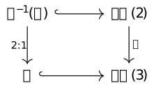
For any of the three rotation groups \(R\), the square records the subgroup and its central double cover. In particular, the Hurwitz-unit model of \(2T\) is this tetrahedral preimage. Its quaternion generators \(i,j,k\) and \((-1+i+j+k)/2\) preserve the 4 imaginary vectors \((1,1,1)\), \((1,-1,-1)\), \((-1,1,-1)\), \((-1,-1,1)\): the first generators change two coordinate signs, and the last cyclically permutes coordinates. Its 24 elements therefore exhaust the preimage. This identifies the group used in the finite spinor gauge example.
TauCeti's
Quaternion.unitaryEquivSpecialUnitaryGroup
formalizes precisely the group equivalence between unit Hamilton
quaternions and \(SU(2)\), using the displayed matrix map. This
correspondence does not assert the \(SO(3)\) quotient or the three
binary subgroup identifications; those have their separate arguments
above. A finite subgroup supplies an available group action, not a
physical interpretation of that action.
Definition 30.9. A representation datum for a field [fdip-007H]AGENTDRAFTED
- November 1, 2026
Definition 30.9. A representation datum for a field [fdip-007H]AGENTDRAFTED
- November 1, 2026
A representation datum specifies a finite discrete or compact Hausdorff group \(G\), a scalar field \(\mathbb K\in \{\mathbb R,\mathbb C\}\), a finite-dimensional fiber \(F\) over \(\mathbb K\), a continuous representation \(\rho :G\to GL_{\mathbb K}(F)\), and a separately chosen action \(\alpha :G\to \operatorname {Aut}(X)\) on the finite substrate \(X\). The substrate automorphisms preserve the graph, weights and any supplied oriented cell data, with orientation changes interpreted by the established inverse-transport convention. One must also specify a positive invariant real or Hermitian inner product on \(F\). The field itself is a map \(\phi :V\to F\).
An invariant inner product always exists for these groups. From any positive inner product \(h_0\), define \[h(v,w)=\int _G h_0(\rho (g)v,\rho (g)w)\,d\mu _G(g).\] The normalized Haar measure makes this invariant by a change of variable. The integral is finite by compactness, and \(h(v,v)>0\) for \(v\ne 0\), since \(\rho (g)v\ne 0\) for every \(g\). This proves existence of an invariant metric; it does not make that metric a canonical choice. A selected metric remains part of the background data.
The global action associated to the datum is \[(g\cdot \phi )(v)=\rho (g)\phi (\alpha (g)^{-1}v).\] The two actions have different roles. For a purely internal group, \(\alpha \) is trivial: the group acts on values without moving vertices. A local gauge transformation instead assigns an element \(g_v\) independently at each vertex and transforms links by \(U_e\mapsto g_{h(e)}U_eg_{s(e)}^{-1}\). It fixes the substrate; a global substrate action \(\alpha \) cannot simply be applied independently at each vertex.
If a field has an additional spin space \(S\), an internal action on \(S\otimes F\) is \(1_S\otimes \rho (g)\). Clifford operators \(\gamma _j\otimes 1_F\) then commute with that action because they act on different factors. An identification of internal and spin symmetries, or an action moving the substrate, needs extra compatible data; it is not implied by the abstract group name or by an inclusion in \(SU(2)\).
Example 30.10. Two fibers for binary tetrahedral symmetry [fdip-007K]AGENTDRAFTED
- November 1, 2026
Example 30.10. Two fibers for binary tetrahedral symmetry [fdip-007K]AGENTDRAFTED
- November 1, 2026
Take the binary tetrahedral group and a fixed finite substrate, with trivial substrate action in the representation datum. Its spinor datum uses \(\mathbb K=\mathbb C\), \(F=\mathbb C^2\) with its standard Hermitian metric, and the inclusion \(2T\subset SU(2)\). Its rotation datum uses \(\mathbb K=\mathbb R\), \(F=\mathbb R^3\) with its Euclidean metric, and the representation obtained through \(\pi :SU(2)\to SO(3)\).
The latter kills \(\{1,-1\}\), while the former is faithful. Thus these choices define different fibers and observables even though the abstract group and the substrate are the same. The spinor Wilson calculation uses the former. A choice of \(G\) alone would not select that representation.
31. Reflection positivity on a finite time lattice [fdip-007L]AGENTDRAFTED
- November 1, 2026
31. Reflection positivity on a finite time lattice [fdip-007L]AGENTDRAFTED
- November 1, 2026
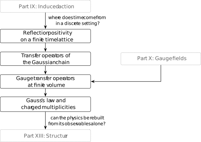
Where could time evolution come from when a law describes all lattice sites at once? Choose one direction to test as Euclidean time. Reflection positivity asks whether observables on one half of the lattice have a positive semidefinite pairing with their reflected partners. Quotienting the vectors of zero length and completing gives a Hilbert space. Reflection positivity is stronger than invariance of the probability law under reflection. The two-site Gaussian makes the sign of a crossing interaction visible.
The scalar result below uses a finite nearest-neighbor torus, reflection-invariant nonnegative weights and positive mass. Its proof first treats a bounded field range, then removes that cutoff. Site reflections retain shared boundary coordinates; link reflections split the sites into disjoint halves. Neither choice makes a time translation an operator on the resulting quotient without further assumptions.
A step of evolution therefore needs more than this positive pairing. The later Gaussian transfer operator uses a nearest-neighbor kernel with positive weight and mass and a specified reference measure; the gauge transfer construction specifies a positive character kernel and gauge projection. Their spectral hypotheses and normalizations permit a Hamiltonian logarithm. These are Euclidean transfer constructions, not an automatic normalized real-time probability evolution.
Definition 31.1. Reflections, halves and the positive-time domain [fdip-007M]AGENTDRAFTED
- November 1, 2026
Definition 31.1. Reflections, halves and the positive-time domain [fdip-007M]AGENTDRAFTED
- November 1, 2026
Let \(Y\) be a finite spatial torus with coordinate periods at least three, or a point. Put \(X=Y\times \mathbb Z/(2M)\), where \(M\ge 2\); the second coordinate is the chosen time direction. The nearest-neighbor graph joins sites differing by one coordinate step, with each undirected edge counted once. Time indices below are taken modulo \(2M\). Define the site reflection and link reflection by \[\theta _s(y,t)=(y,-t),\qquad \theta _\ell (y,t)=(y,1-t).\] Their positive halves and fixed sets are \[\begin {aligned} X_+^s&=Y\times \{0,\ldots ,M\},& X_0^s&=Y\times \{0,M\},\\ X_+^\ell &=Y\times \{1,\ldots ,M\},& X_0^\ell &=\varnothing . \end {aligned}\] In either case set \(X_-=\theta X_+\). Then \(X_+\cup X_-=X\) and \(X_+\cap X_-=X_0\); sites in \(X_0\) are fixed individually.
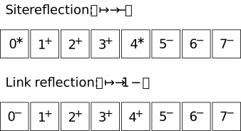
The diagram shows one time circle of length 8. A plus or minus marks an interior site of that half; a star marks a fixed site shared by both halves. Time \(7\) is adjacent to time \(0\). The boxes display membership in the halves, not separate field copies.
For a real scalar configuration \(\phi \in \mathbb R^X\), write \((\theta \phi )_v=\phi _{\theta v}\). On complex observables define \[(\Theta f)(\phi )=\overline {f(\theta \phi )}.\] Thus \(\Theta \) is an antilinear multiplicative involution. Let \(\mathcal A_+\) be the algebra of bounded complex measurable functions depending only on \(\phi |_{X_+}\). Let \(\mu \) be a probability measure on \(\mathbb R^X\). Reflection invariance means \(\theta _*\mu =\mu \). In addition, reflection positivity means \[B_\mu (f,f):=\int (\Theta f)f\,d\mu \ge 0 \qquad (f\in \mathcal A_+).\] The inequality includes the assertion that the integral is real. Under reflection invariance, \(B_\mu (f,g)=\int (\Theta f)g\,d\mu \) is Hermitian and conjugate-linear in its first argument. These are the complex-observable conventions corresponding to [friedli2017statistical, Definition 10.5, p. 441].
The larger positive-time domain is \(\mathcal H_+=L^2(\mathbb R^X,\mu ;\mathbb C)\) restricted to functions measurable in the coordinates of \(X_+\). It is a closed vector subspace, generally not an algebra under pointwise multiplication. Reflection invariance gives \[|B_\mu (f,g)|\le \|f\|_{L^2(\mu )}\|g\|_{L^2(\mu )}.\] Truncating the values of a function shows that \(\mathcal A_+\) is dense in \(\mathcal H_+\). Consequently positivity on \(\mathcal A_+\) extends to this domain. For a reflection-positive law, the quotient by \(\mathcal N=\{f:B_\mu (f,f)=0\}\), with the induced pairing, has a Hilbert-space completion. This definition supplies no translation operator on that quotient.
Lemma 31.2. A sufficient positive-half decomposition [fdip-007N]AGENTDRAFTED
- November 1, 2026
Lemma 31.2. A sufficient positive-half decomposition [fdip-007N]AGENTDRAFTED
- November 1, 2026
Let a finite set \(X\) have an involution \(\theta \) and halves \(X_-=\theta X_+\) with \(X_+\cup X_-=X\) and \(X_+\cap X_-=\operatorname {Fix}(\theta )=X_0\). Use the observable conventions of Definition 31.1; both torus reflections there have these properties. Let \(\nu \) be a probability measure supported on a compact interval of \(\mathbb R\), and put \(\mu _0=\bigotimes _{v\in X}\nu \). Suppose a real Hamiltonian has the form \[-H=A+\Theta A+\sum _{\alpha =1}^q C_\alpha \Theta C_\alpha ,\] where \(A,C_1,\ldots ,C_q\) are bounded real functions in \(\mathcal A_+\); the sum may be empty. Then the probability law \[d\mu =Z^{-1}e^{-H}\,d\mu _0,\qquad Z=\int e^{-H}\,d\mu _0\] is reflection invariant and reflection positive. This is the complex-observable version of [friedli2017statistical, Lemma 10.8, pp. 442–443].
Proof.
- November 1, 2026
Proof.
- November 1, 2026
First consider the product reference. Conditional on the field \(b=\phi |_{X_0}\) at the fixed sites, the two interiors are independent and have matching product laws under reflection. The boundary field is a single shared variable. For any bounded positive-half observable \(F\), therefore, \[\int (\Theta F)F\,d\mu _0 =\int \left |\int F(\phi _+,b)\,d\nu _+(\phi _+)\right |^2 \,d\nu _0(b)\ge 0.\] Here \(\nu _+\) is the product over \(X_+\setminus X_0\) and \(\nu _0\) the product over \(X_0\). When \(X_0\) is empty the outer integral is evaluation at the unique empty configuration. This also proves the product case of [friedli2017statistical, Lemma 10.7, p. 442].
The displayed decomposition is invariant under reflection because its functions are real and multiplication commutes. The reference law is invariant as well. Boundedness makes \(0<Z<\infty \) and permits uniform absolute expansion of the crossing exponential. For \(f\in \mathcal A_+\), this gives \[\begin {aligned} ZB_\mu (f,f) &=\sum _{n\in \mathbb N^q}\frac 1{n!} B_{\mu _0}\left (fe^A C^n,fe^A C^n\right ),\\ n!&=\prod _\alpha n_\alpha !,\qquad C^n=\prod _\alpha C_\alpha ^{n_\alpha }. \end {aligned}\] Every summand is nonnegative by the conditional product identity. The sum converges absolutely by the bounded exponential majorant, so the claimed positivity follows.
Theorem 31.3. Reflection positivity of a massive scalar lattice [fdip-007O]AGENTDRAFTED
- November 1, 2026
Theorem 31.3. Reflection positivity of a massive scalar lattice [fdip-007O]AGENTDRAFTED
- November 1, 2026
On the nearest-neighbor torus of Definition 31.1, choose either reflection \(\theta \). Give every undirected edge a nonnegative weight \(w_e\) with \(w_{\theta e}=w_e\), and fix \(m>0\). The real scalar law \[\begin {aligned} H(\phi )&=\frac 12\sum _{e=\{u,v\}}w_e(\phi _u-\phi _v)^2 +\frac {m^2}{2}\sum _{v\in X}\phi _v^2,\\ d\mu (\phi )&=Z^{-1}e^{-H(\phi )} \prod _{v\in X}d\phi _v \end {aligned}\] is reflection invariant and reflection positive on \(\mathcal A_+\) and its positive-time \(L^2\) domain. Every polynomial in the positive-half field coordinates belongs to that domain. This is the massive scalar precision with zero-weight edges omitted. It uses ordinary differences, equivalently trivial transport in the connection energy.
Proof.
- November 1, 2026
Proof.
- November 1, 2026
Since \(H(\phi )\ge (m^2/2)\|\phi \|^2\), the normalizer is finite and positive, and every polynomial moment exists. Reflection is a permutation of the coordinates, preserves Lebesgue measure and preserves \(H\) by the weight hypothesis. This proves invariance separately from positivity.
For a site reflection, no nearest-neighbor edge joins \(X_+\setminus X_0\) directly to \(X_-\setminus X_0\). Partition the terms of \(H\) into \(H_+\), those supported in \(X_+\) but not wholly in \(X_0\); their reflected partners \(H_-=\Theta H_+\); and \(H_0\), those supported wholly in \(X_0\). Include onsite mass terms in the same partition. Because reflection fixes every boundary coordinate, \[-H=A+\Theta A,\qquad A=-H_+-\tfrac 12H_0.\] In particular the boundary terms are counted once.
For a link reflection the halves are disjoint. The only crossing edges are the time bonds at the two cuts, and each has the form \(e=\{v,\theta v\}\) with a unique \(v\in X_+\). Its contribution to \(-H\) is \[-\frac {w_e}{2}\phi _v^2 -\frac {w_e}{2}\phi _{\theta v}^2 +w_e\phi _v\phi _{\theta v}.\] Put its first term into \(A\), its second into \(\Theta A\), and write the last as \(C_e\Theta C_e\), where \(C_e=\sqrt {w_e}\phi _v\). All within-half edge energies and onsite mass terms are assigned to their own half, with a minus sign. Reflection invariance of the weights then gives the positive-half decomposition.
For \(R>0\), restrict every coordinate to \([-R,R]\) and use the uniform probability on this interval as the product reference. On that cube the functions \(A,C_e\) are bounded, so the lemma proves reflection positivity of the normalized cutoff law \(\mu _R\). The constant reference-density factor cancels from normalization; thus \(\mu _R\) is exactly \(\mu \) conditioned on \(\max _v|\phi _v|\le R\). For bounded \(f,g\), dominated convergence in the integrable Gaussian density gives \[B_{\mu _R}(f,g)\longrightarrow B_\mu (f,g).\] For polynomials the same argument uses a polynomial times the dominating massive Gaussian. In particular positivity survives the limit. Finally, bounded value truncations are dense in \(\mathcal H_+\); the norm bound in Definition 31.1 extends the pairing and its positivity to all of that domain.
Compare [friedli2017statistical, pp. 443–444], Examples 10.9–10.10, for the half decompositions. The cutoff argument above supplies the noncompact Gaussian step. Arbitrary inhomogeneous weights need not respect the chosen reflection. Arbitrary fixed connections need not have the displayed nonnegative crossing terms. Neither case is asserted by this theorem.
Example 31.4. The two-site reflection Gram matrix [fdip-007P]AGENTDRAFTED
- November 1, 2026
Example 31.4. The two-site reflection Gram matrix [fdip-007P]AGENTDRAFTED
- November 1, 2026
Take two real field coordinates \(x,y\), interchanged by reflection, and the centered Gaussian precision \[Q=\begin {pmatrix}a&-w\\-w&a\end {pmatrix}, \qquad a>|w|.\] The positive-half observables depend on \(x\). The covariance is \[G=Q^{-1} =\frac 1{a^2-w^2}\begin {pmatrix}a&w\\w&a\end {pmatrix}.\] For \(a=2,w=1\), this becomes \[G=\begin {pmatrix}2/3&1/3\\1/3&2/3\end {pmatrix}.\] The energy has positive mass squared \(a-w=1\) and crossing weight \(w=1\), so the same cutoff criterion proves reflection positivity.
For \(f_0=1,f_1=x,f_2=x^2\), the reflection Gram matrix is \[\left (B_\mu (f_j,f_k)\right )_{j,k=0}^2 =\begin {pmatrix} 1&0&2/3\\ 0&1/3&0\\ 2/3&0&2/3 \end {pmatrix}.\] Odd Gaussian moments vanish, and \(\mathbb E[x^2y^2]=(2/3)^2+2(1/3)^2=2/3\) by the four-factor Gaussian calculation. The leading principal minors are \(1\), \(1/3\) and \(2/27\), so this finite Gram matrix is positive definite. Positivity of this one matrix is an illustration; the criterion proves the claim for all positive-half observables.
TauCeti's
TauCeti.Probability.integral_mul_mul_mul_multivariateGaussian
proves the fourth-moment identity for a finite coordinate index set
and a positive-semidefinite covariance, including repeated indices.
Apply it with the displayed \(G\) and indices \(x,x,y,y\).
This correspondence supports the moment calculation; the reflected
pairing and its Gram-matrix positivity are computed here.
If instead \(a=2,w=-1\), the precision remains positive definite and its Gaussian remains reflection invariant. But \[B_\mu (x,x)=\mathbb E[xy]=-\frac 13<0.\] Thus reflection invariance and ordinary Gaussian positivity do not imply reflection positivity. The witness \(x\) is square-integrable; bounded value truncations also have a negative pairing once the cutoff is large enough, by continuity of \(B_\mu \).
Example 31.5. Reflection positivity without a quotient time shift [fdip-007Q]AGENTDRAFTED
- November 1, 2026
Example 31.5. Reflection positivity without a quotient time shift [fdip-007Q]AGENTDRAFTED
- November 1, 2026
On time sites \(\mathbb Z/6\), let \(\phi _t\) be independent centered real Gaussians with variances \[(v_0,v_1,v_2,v_3,v_4,v_5)=(1,1,2,3,3,2).\] Use the link reflection \(\theta (t)=1-t\) and positive half \(X_+=\{1,2,3\}\). Since \(v_{\theta t}=v_t\), the product law is reflection invariant. The halves are independent and their laws agree under reflection, so for every positive-half square-integrable \(F\), \[B_\mu (F,F)=|\mathbb E_\mu F|^2\ge 0.\] This proves reflection positivity directly, without a translation-invariance assumption.
Define a one-step shift of a coordinate expression by replacing each \(\phi _t\) by \(\phi _{t+1}\). On expressions whose sites remain in \(X_+\), this at least gives another positive-half function. In particular, \[F=\phi _1^2-1,\qquad \tau F=\phi _2^2-1\] both belong to the positive-time \(L^2\) domain. Their pairings are \[B_\mu (F,F)=0,\qquad B_\mu (\tau F,\tau F)=1.\] Indeed their expectations are \(v_1-1=0\) and \(v_2-1=1\). The centering constant is part of the shifted expression and does not change from \(1\) to \(v_2\).
Thus a zero vector in the reflection quotient would be sent to a nonzero one. The shift cannot descend even on this pair of positive-half polynomials. A transfer operator requires additional structure; reflection positivity alone does not construct it.
Remark 31.6. The scalar result and the gauge transfer question [fdip-007R]AGENTDRAFTED
- November 1, 2026
Remark 31.6. The scalar result and the gauge transfer question [fdip-007R]AGENTDRAFTED
- November 1, 2026
The sufficient criterion here comes from the compact-spin argument of Friedli–Velenik [friedli2017statistical, Lemma 10.8, pp. 442–443], with an explicit Gaussian cutoff passage. It concerns an ordinary scalar field with a chosen reflection. The classical small-spacing expansion of the Wilson action supplies no reflection-positive probability law by itself. Nor does integrating matter into a connection marginal establish such a property.
For gauge fields, the positive-character kernel conditions give a different starting point for an explicit finite-volume transfer construction. One must specify the convolution kernel, gauge projection and time-boundary convention and prove the operator properties. The failure of a quotient shift explains why those steps cannot be replaced by reflection positivity alone.
Osterwalder–Seiler [osterwalder1978gauge] provides historical context for gauge and fermion positivity. It is cited here for that context only; no theorem or proof from it is used to extend the scalar result. General gauge–fermion reflection positivity, an infinite-time vacuum construction and continuum reconstruction require separate hypotheses and arguments. Time here remains a chosen lattice direction, rather than an additional field observable.
32. Transfer operators of the Gaussian chain [fdip-007S]AGENTDRAFTED
- November 1, 2026
32. Transfer operators of the Gaussian chain [fdip-007S]AGENTDRAFTED
- November 1, 2026
A nearest-neighbor Gaussian energy factors into kernels between successive time slices. Composing those kernels gives a transfer operator; closing the chain gives its trace. For a single real field per slice, Hermite functions diagonalize the operator exactly. The leading eigenvalue fixes the normalization needed before its logarithm becomes a nonnegative Hamiltonian.
The construction uses positive weight and mass, Lebesgue measure on each field coordinate and a unit time step. It supplies the operator structure that reflection positivity alone does not determine. The cycle determinant and periodic covariance give independent finite-dimensional checks of its partition function and field correlations.
Definition 32.1. The one-step Gaussian kernel [fdip-007T]AGENTDRAFTED
- November 1, 2026
Definition 32.1. The one-step Gaussian kernel [fdip-007T]AGENTDRAFTED
- November 1, 2026
Fix \(w>0\) and \(m>0\). On \(\mathcal H=L^2(\mathbb R,dx;\mathbb C)\), define the Gaussian transfer operator by \[\begin {aligned} K(x,y)&=\exp \left [-\frac w2(x-y)^2 -\frac {m^2}{4}(x^2+y^2)\right ],\\ (Tf)(x)&=\int _{\mathbb R}K(x,y)f(y)\,dy. \end {aligned}\] The reference measure is exactly Lebesgue measure \(dy\); no normalizing factor is included in \(K\). This is the one-coordinate instance of the slice-kernel construction in [wingate2025lattice, Eqs. (5.1)–(5.3), p. 4].
Write \(a=w/2+m^2/4\), so \(K(x,y)=e^{-a(x^2+y^2)+wxy}\) and \(2a>w\). Thus \(K\in L^2(\mathbb R^2)\). Cauchy–Schwarz makes \(T\) bounded, and symmetry of the real kernel makes it self-adjoint. An integral operator with a square-integrable kernel is Hilbert–Schmidt: in an orthonormal basis \((e_n)\), its squared norm of this kind is \(\|T\|_{\mathrm {HS}}^2=\sum _n\|Te_n\|^2\) (the value is independent of the basis). Here it equals \(\int |K|^2\). Approximation of \(K\) by finite sums of products of one-variable square-integrable functions also shows that \(T\) is compact. Operator positivity will follow from its explicit spectrum in Theorem 32.2.
For \(N\ge 3\), let \(x_N=x_0\) and define the periodic chain by \[\begin {aligned} H_N(x)&=\frac w2\sum _{j=0}^{N-1}(x_{j+1}-x_j)^2 +\frac {m^2}{2}\sum _{j=0}^{N-1}x_j^2,\\ Z_N&=\int _{\mathbb R^N}e^{-H_N(x)}\,d^Nx,\qquad d\mu _N=Z_N^{-1}e^{-H_N(x)}\,d^Nx. \end {aligned}\] Each undirected edge of the ordinary cycle \(C_N\) occurs once. Splitting each onsite mass term between its two incident edges gives \[e^{-H_N(x)}=\prod _{j=0}^{N-1}K(x_j,x_{j+1}).\] Positive mass makes \(0<Z_N<\infty \). The identity \(Z_N=\operatorname {Tr}T^N\) is proved in Theorem 32.4.
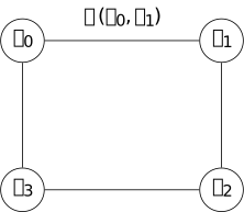
The four-cycle illustrates the kernel product. Every edge contributes the same function \(K\) of its endpoints. Each site's two mass contributions add to \(m^2x_j^2/2\); closing the last edge identifies \(x_4\) with \(x_0\).
Theorem 32.2. Hermite diagonalization [fdip-007U]AGENTDRAFTED
- November 1, 2026
Theorem 32.2. Hermite diagonalization [fdip-007U]AGENTDRAFTED
- November 1, 2026
For the Gaussian transfer operator, define \[\begin {aligned} \cosh \omega &=1+\frac {m^2}{2w},& \omega &>0,\\ q&=e^{-\omega },& s&=w\sinh \omega ,\\ \lambda _0&=\sqrt {\frac {2\pi }{w}}e^{-\omega /2}. \end {aligned}\] Define the probabilists' Hermite polynomials \(\operatorname {He}_n\) by the generating function \[e^{uz-z^2/2} =\sum _{n=0}^\infty \operatorname {He}_n(u)\frac {z^n}{n!},\] and put \[h_n^s(x)=\left (\frac {s}{\pi }\right )^{1/4} \frac {\operatorname {He}_n(\sqrt {2s}\,x)}{\sqrt {n!}} e^{-sx^2/2}.\] These functions form an orthonormal basis of \(L^2(\mathbb R,dx;\mathbb C)\), and \[Th_n^s=\lambda _0q^nh_n^s\qquad (n\ge 0).\] Consequently \(T\) is positive, injective and trace class, with \(\|T\|=\lambda _0\) and \(\operatorname {Tr}T=\lambda _0/(1-q)\). The normalized operator \(\widehat T=T/\lambda _0\) is an injective positive contraction.
Proof.
- November 1, 2026
Proof.
- November 1, 2026
First establish the basis. Integrating two generating functions against \(e^{-sx^2}\) gives \[\begin {aligned} &\int _{\mathbb R}e^{-sx^2} e^{\sqrt {2s}\,xz-z^2/2} e^{\sqrt {2s}\,xt-t^2/2}\,dx\\ &\hspace {20mm}=\sqrt {\frac \pi s}\,e^{zt}. \end {aligned}\] Differentiation at \(z=t=0\) proves orthogonality with precisely the displayed normalization. Every such differentiation is justified by a polynomial times an integrable Gaussian, uniformly for the complex parameters in a compact set.
For completeness, suppose \(f\in L^2\) is orthogonal to every \(h_n^s\). Since \(\operatorname {He}_n\) has degree \(n\) and leading coefficient one, all moments of \(g(x)=f(x)e^{-sx^2/2}\) vanish. Cauchy–Schwarz shows that \(g\in L^1\) and that \[F(z)=\int _{\mathbb R}g(x)e^{zx}\,dx\] is entire: on every compact set of complex \(z\), all derivative integrands have an integrable majorant of the form \(|f(x)|\,|x|^k e^{-sx^2/2+R|x|}\). All Taylor coefficients of \(F\) vanish, so \(F=0\); in particular the Fourier transform of \(g\) vanishes. To see the needed uniqueness directly, convolve \(g\) with a normalized Gaussian. The Gaussian Fourier integral and Fubini express this convolution as an integral of its zero Fourier transform, hence it is zero. As the Gaussian variance tends to zero, these convolutions tend to \(g\) in \(L^1\), by continuity of translations in \(L^1\) and dominated convergence. Thus \(g=0\) almost everywhere and \(f=0\). The orthonormal family is complete.
Now diagonalize the kernel. With \(a=w\cosh \omega /2\), the identities \(s=w\sinh \omega \) and \(a+s/2=w/(2q)\) give, by completing the square in \(y\), \[\begin {aligned} &\int _{\mathbb R}K(x,y)e^{-sy^2/2} e^{\sqrt {2s}\,yz-z^2/2}\,dy\\ &\hspace {8mm}=\lambda _0e^{-sx^2/2} e^{\sqrt {2s}\,xqz-q^2z^2/2}. \end {aligned}\] The constant is \(\sqrt {\pi /(a+s/2)}=\sqrt {2\pi q/w}=\lambda _0\). Differentiating \(n\) times at zero, again under a Gaussian majorant, gives \(Th_n^s=\lambda _0q^nh_n^s\).
If \(f=\sum _n c_nh_n^s\), boundedness and completeness give \[Tf=\sum _{n=0}^\infty \lambda _0q^nc_nh_n^s\] in \(L^2\). Every eigenvalue is strictly positive, which proves positivity and injectivity. Their maximum is \(\lambda _0\). For a positive compact operator, being trace class means that these eigenvalues have finite sum; here the sum is \(\lambda _0/(1-q)\). This proves all operator assertions. It also gives the Mehler kernel expansion \[K(x,y)=\sum _{n=0}^\infty \lambda _0q^nh_n^s(x)h_n^s(y)\] in \(L^2(\mathbb R^2)\): the squared Hilbert–Schmidt norm of the tail is \(\lambda _0^2\sum _{n>r}q^{2n}\) after truncation at \(r\). This convergence statement suffices for the operator identity.
The calculation is a direct diagonalization of
Definition 32.1. TauCeti's
TauCeti.hermiteHilbertBasis and
TauCeti.coe_hermiteHilbertBasis
supply the complete orthonormal Hermite basis at \(s=1\), with
exactly the probabilists' normalization used here. The unitary
dilation \(f(x)\mapsto s^{1/4}f(\sqrt {s}\,x)\) gives the displayed
basis for general \(s>0\). These references support the basis;
the kernel eigenvalues and transfer properties are proved above.
Example 32.3. A transfer norm greater than one [fdip-007X]AGENTDRAFTED
- November 1, 2026
Example 32.3. A transfer norm greater than one [fdip-007X]AGENTDRAFTED
- November 1, 2026
Take \(w=3/2\) and \(m^2=4/5\) in Theorem 32.2. Then \[\begin {aligned} \cosh \omega &=\frac {19}{15},& s&=\frac {\sqrt {34}}5,\\ q&=\frac {19-2\sqrt {34}}{15},& \lambda _0&=\sqrt {\frac {4\pi q}{3}}. \end {aligned}\] Numerically \(\omega \approx 0.714971\) and \(\lambda _0\approx 1.431497\). In particular \(\|T\|=\lambda _0>1\). This inequality does not depend on rounding: \(\sqrt {34}<6\) gives \(q>7/15\), and \(\pi >3\) gives \(\lambda _0^2>28/15>1\).
All eigenvalues are nevertheless positive: \(\lambda _n=\lambda _0q^n\). Dividing by the leading eigenvalue gives \(\widehat T h_n^s=q^nh_n^s\) and \(\|\widehat T\|=1\). The lowest mode label \(n=0\) refers to the Gaussian function \(h_0^s\), not to a constant function on \(\mathbb R\); the latter does not belong to Lebesgue \(L^2\). Thus the normalization is a genuine scalar factor in the operator, fixed by the chosen reference measure.
Theorem 32.4. Periodic traces and field correlations [fdip-007V]AGENTDRAFTED
- November 1, 2026
Theorem 32.4. Periodic traces and field correlations [fdip-007V]AGENTDRAFTED
- November 1, 2026
Use the kernel and parameters of Definition 32.1 and Theorem 32.2. For every integer \(N\ge 1\), \[\operatorname {Tr}T^N =\frac {\lambda _0^N}{1-q^N} =\frac {(2\pi /w)^{N/2}}{2\sinh (N\omega /2)}.\] For \(N\ge 3\), this equals the periodic Gaussian normalizer \(Z_N\). If \(f_0,\ldots ,f_{N-1}\) are bounded complex measurable functions and \(M_f\) denotes multiplication by \(f\), then \[\mathbb E_{\mu _N}\prod _{j=0}^{N-1}f_j(x_j) =\frac {\operatorname {Tr} (M_{f_0}T M_{f_1}T\cdots M_{f_{N-1}}T)}{Z_N}.\] In particular, bounded two-point observables have the usual cyclic trace expression with \(T^{N-t}\) and \(T^t\).
For \(N\ge 3\) and the unbounded coordinate observable, let \(Xf(x)=xf(x)\) on its domain \(\{f\in L^2:xf\in L^2\}\). For integers \(0\le t\le N\), initially on finite Hermite sums, put \[A_t=T^{t/2}XT^{(N-t)/2}.\] It has a unique Hilbert–Schmidt extension. The precise coordinate trace formula is \[\begin {aligned} \mathbb E_{\mu _N}[x_0x_t] &=\frac {\operatorname {Tr}(A_t^*A_t)}{Z_N}\\ &=\frac {q^t+q^{N-t}}{2s(1-q^N)}, \qquad x_N=x_0. \end {aligned}\] Here \(\operatorname {Tr}(A_t^*A_t)\) supplies the meaning of the frequently written unbounded expression \(\operatorname {Tr}(T^{N-t}XT^tX)\).
Proof.
- November 1, 2026
Proof.
- November 1, 2026
The eigenvalues in Theorem 32.2 give the first trace by a geometric sum. The remaining expression uses \(\lambda _0=\sqrt {2\pi /w}\,q^{1/2}\) and \(q^{-N/2}-q^{N/2}=2\sinh (N\omega /2)\). On the ordinary cycle, the precision is \(Q_N=m^2I+wL_{C_N}\). The twisted-cycle determinant at trivial holonomy, with the scalar factor \(w\) restored, gives \[\det Q_N=w^N\bigl (2\cosh (N\omega )-2\bigr ).\] The real Gaussian integral therefore gives exactly the same \(Z_N\). The trace identity for \(N=1,2\) remains an operator identity; no ordinary simple-cycle identification is used for those two periods.
For bounded insertions, \(M_fT\) is Hilbert–Schmidt. The product of two such operators is trace class; multiplying by the remaining bounded factors preserves this property. The Hilbert–Schmidt kernel trace identity \[\operatorname {Tr}(AB)=\int _{\mathbb R^2}A(x,y)B(y,x)\,dx\,dy\] follows by expanding the two kernels in an orthonormal basis and taking their \(L^2\) pairing. Applying it to the cyclic product and composing the intervening kernels yields \[\operatorname {Tr}(M_{f_0}T\cdots M_{f_{N-1}}T) =\int _{\mathbb R^N}\prod _j f_j(x_j) \prod _jK(x_j,x_{j+1})\,d^Nx.\] All repeated integrals are absolutely convergent: the absolute integrand is bounded by \(\prod _j\|f_j\|_\infty \) times the integrable massive Gaussian. The kernel factorization in Definition 32.1 proves the asserted expectation.
For the coordinate insertion, the Hermite generating function gives the recurrence \[Xh_n^s=\frac {\sqrt {n+1}\,h_{n+1}^s +\sqrt n\,h_{n-1}^s}{\sqrt {2s}},\] where the second term is zero at \(n=0\). Consequently the matrix of \(A_t\) has only two adjacent diagonals. Summing their squared entries gives \[\begin {aligned} \|A_t\|_{\mathrm {HS}}^2 &=\frac {\lambda _0^N}{2s} \frac {q^t+q^{N-t}}{(1-q^N)^2}. \end {aligned}\] The sum is finite also at \(t=0,N\). Thus the operator on the dense finite Hermite span extends uniquely to a Hilbert–Schmidt operator. Thus \(A_t^*A_t\) is positive trace class and its trace is this squared norm. Division by \(Z_N\) gives the displayed value. Finally, the periodic covariance calculation, with \(s=w\sinh \omega \), gives this same value for \((Q_N^{-1})_{0t}\). Gaussian covariance therefore identifies it with \(\mathbb E_{\mu _N}[x_0x_t]\), including the periodic endpoint. No cyclic manipulation of an undefined unbounded product is used.
This finite periodic calculation makes the trace notation of [wingate2025lattice, Eq. (5.4), p. 4] explicit for the Gaussian chain. That source subsequently takes an infinite-time limit; the identities here hold at finite \(N\). The Ising transfer and Markov-chain comparison in [friedli2017statistical, Section 3.10.4, p. 139] concerns a different state space and is background for the transfer interpretation, not a premise for this Gaussian proof.
Corollary 32.5. The oscillator Hamiltonian [fdip-007W]AGENTDRAFTED
- November 1, 2026
Corollary 32.5. The oscillator Hamiltonian [fdip-007W]AGENTDRAFTED
- November 1, 2026
For the normalized transfer operator \(\widehat T=T/\lambda _0\) of Theorem 32.2, the transfer Hamiltonian is the spectral logarithm \(H=-\log \widehat T\). Explicitly, if \(f=\sum _{n\ge 0}c_nh_n^s\), its domain and action are \[\begin {aligned} D(H)&=\left \{f:\sum _{n=0}^\infty (n\omega )^2|c_n|^2<\infty \right \},\\ Hf&=\sum _{n=0}^\infty n\omega c_nh_n^s. \end {aligned}\] It is nonnegative and self-adjoint, with eigenvalues \(n\omega \). Its zero eigenspace is the line spanned by \(h_0^s\), and its mass gap is \(\omega \). It is unbounded even though \(\widehat T\) is bounded and injective.
On the finite Hermite span, it has the differential expression \[Hf=\frac \omega {2s} \left (-f''+s^2x^2f-sf\right ).\] The closure of this expression on that span is the above spectral operator. This is the harmonic oscillator with its ground energy subtracted. The time step has length one; a specified step \(a_t>0\) instead gives \(H/a_t\) and gap \(\omega /a_t\).
Proof.
- November 1, 2026
Proof.
- November 1, 2026
The unitary coefficient map \(f\mapsto (c_n)\) identifies \(\widehat T\) with multiplication by \(q^n>0\) on \(\ell ^2\). Its negative logarithm is multiplication by \(n\omega \) on the stated maximal domain. A real diagonal operator on that domain is self-adjoint; its quadratic form is nonnegative. The listed eigenspaces, spectrum and gap follow directly, and \(\|Hh_n^s\|=n\omega \) proves unboundedness. Finite coefficient truncations converge both in norm and after applying \(H\), so the finite Hermite span is a core.
Differentiating the Hermite generating function and comparing coefficients gives \(\operatorname {He}_n''(u)-u\operatorname {He}_n'(u) +n\operatorname {He}_n(u)=0\). Substitution into the definition of \(h_n^s\) yields \[-(h_n^s)''+s^2x^2h_n^s=(2n+1)s\,h_n^s.\] The displayed differential expression therefore acts as \(n\omega \) on every basis vector. The core statement proves that its closure is exactly \(H\).
TauCeti's
TauCeti.hermiteFunction_oscillator
proves the pointwise differential identity at \(s=1\) for the
same normalized Hermite functions. Dilation gives the identity
above for \(s>0\); the spectral logarithm, its domain and the
closure statement are supplied by the preceding argument.
The logarithmic prescription follows [wingate2025lattice, Eq. (5.5), p. 4], with the leading transfer eigenvalue removed explicitly. It constructs the Hamiltonian for a Gaussian model of finite spatial volume. No limit in time, spatial volume or lattice spacing is needed.
33. Gauge transfer operators at finite volume [fdip-007Y]AGENTDRAFTED
- November 1, 2026
33. Gauge transfer operators at finite volume [fdip-007Y]AGENTDRAFTED
- November 1, 2026
A positive character expansion turns a temporal plaquette weight into a positive operator on spatial link fields. Multiplication by half of the spatial weight on each side gives a transfer operator. Gauge averaging selects its physical states and retains the temporal links when the time direction closes into a circle.
The construction uses a finite spatial graph, normalized Haar measure and the positive kernel hypotheses. It proves finite periodic-time trace identities, a spectral Hamiltonian and link-reflected positivity for bounded spatial observables. The Gaussian transfer construction supplies the scalar comparison; reflection positivity by itself does not supply these operator and translation data.
Definition 33.1. Spatial link fields and their transfer kernel [fdip-007Z]AGENTDRAFTED
- November 1, 2026
Definition 33.1. Spatial link fields and their transfer kernel [fdip-007Z]AGENTDRAFTED
- November 1, 2026
Let \(G\) be a finite group, \(U(1)\) or \(SU(2)\), with normalized Haar measure. Fix a finite incidence presentation with vertex set \(V_s\), oriented edge set \(E_s\) and source and target maps \(s,t:E_s\to V_s\). The spatial configuration space and link Hilbert space are \[X=G^{E_s},\qquad \mathcal H_{\mathrm {link}}=L^2(X,dU;\mathbb C),\] where \(dU\) is product Haar probability measure. The gauge action of \(K=G^{V_s}\) is \[(h\cdot U)_e=h_{t(e)}U_eh_{s(e)}^{-1},\qquad (R_hf)(U)=f(h^{-1}\cdot U).\] Haar invariance makes every \(R_h\) unitary.
Choose a real continuous central kernel \(k\) satisfying the positive coefficient conditions: \[\begin {gathered} k(g)>0,\qquad k(g^{-1})=k(g),\\ k(g)=\sum _{\rho \in \widehat G}d_\rho a_\rho \chi _\rho (g), \qquad a_\rho >0,\qquad \sum _{\rho \in \widehat G}d_\rho ^2a_\rho <\infty . \end {gathered}\] All irreducible representations here are complex and unitary. The expansion is uniformly absolutely convergent. Pointwise positivity and coefficient positivity are separate hypotheses.
Let \(V:X\to \mathbb R\) be continuous and gauge invariant, and set \(b(U)=e^{-V(U)/2}\). Compactness makes \(b\) and \(b^{-1}\) bounded. If \(M_b\) denotes multiplication by \(b\), define \[\begin {aligned} c(U,U')&=\prod _{e\in E_s}k(U_eU_e'^{-1}),\\ (C_kf)(U)&=\int _Xc(U,U')f(U')\,dU',\\ T&=M_bC_kM_b. \end {aligned}\] This is the pure-gauge transfer operator for the specified data. Its integral kernel is \(b(U)c(U,U')b(U')\). The spatial potential may be a sum of Wilson plaquette terms, but the definition only needs its stated invariance and continuity.
The factorization separates the two spatial half-weights from the temporal convolution. It parallels the gauge factors in [luscher1977transfer, Eqs. (17), (20)–(21), p. 287]; the source comparison distinguishes this pure-gauge model from that paper's gauge and fermion construction.
Example 33.2. Positive temporal weights for signs and phases [fdip-0081]AGENTDRAFTED
- November 1, 2026
Example 33.2. Positive temporal weights for signs and phases [fdip-0081]AGENTDRAFTED
- November 1, 2026
The transfer kernel conditions have elementary examples. For \(G=\mathbb Z_2=\{1,-1\}\) and \(\beta >0\), take \(k(u)=e^{\beta u}\). The two characters are \(1\) and \(u\), and \[k(u)=\cosh \beta +u\sinh \beta .\] Thus \(a_{\mathrm {triv}}=\cosh \beta >0\) and \(a_{\mathrm {sgn}}=\sinh \beta >0\). Both dimensions are one, so the coefficient sum is \(e^\beta \). The function is real, strictly positive and invariant under inversion.
For \(G=U(1)\), the Wilson and Villain weights give two choices: \[\begin {aligned} k_W(e^{i\theta })&=e^{\beta \cos \theta }, &a_n^W&=I_n(\beta ),\\ k_V(e^{i\theta })&=\sum _{\ell \in \mathbb Z} e^{-\beta _V(\theta -2\pi \ell )^2/2}, &a_n^V&=\frac {e^{-n^2/(2\beta _V)}}{\sqrt {2\pi \beta _V}}. \end {aligned}\] Here \(\beta ,\beta _V>0\) and \(n\in \mathbb Z\). All coefficients are positive and summable; all characters have dimension one. The cited calculation proves the series, continuity and inversion symmetry. Each function is strictly positive from its definition, so every hypothesis is met. These are unnormalized weights; no zeroth coefficient has been divided out.
At \(\beta =0\), the sign or Wilson weight is constant and its nontrivial Fourier coefficients vanish. The resulting convolution kills nonconstant modes, so strict coefficient positivity cannot be removed from the injectivity assertion in Theorem 33.4.
Proposition 33.3. A positive coefficient expansion on SU(2) [fdip-0082]AGENTDRAFTED
- November 1, 2026
Proposition 33.3. A positive coefficient expansion on SU(2) [fdip-0082]AGENTDRAFTED
- November 1, 2026
Let \(f\) be the defining two-dimensional representation of \(SU(2)\) and \(\beta >0\). Then \[k(g)=e^{\beta \chi _f(g)}\] satisfies the transfer kernel conditions. More precisely, if \(m_\rho (n)\) is the multiplicity of \(\rho \) in \(f^{\otimes n}\), then \[\begin {aligned} c_\rho &=\sum _{n=0}^\infty \frac {\beta ^n}{n!}m_\rho (n)>0,\\ a_\rho &=\frac {c_\rho }{d_\rho },\qquad \sum _\rho d_\rho ^2a_\rho =e^{2\beta }. \end {aligned}\] This is the tensor-power argument used in [luscher1977transfer, Proposition 1, p. 288], with strict occurrence and absolute convergence justified below.
Proof.
- November 1, 2026
Proof.
- November 1, 2026
The matrix description of SU(2) writes its elements as \[g=\begin {pmatrix}z&w\\-\overline w&\overline z\end {pmatrix}, \qquad |z|^2+|w|^2=1.\] Hence \(\chi _f(g)=2\operatorname {Re}z\) is real, \(\chi _f(g^{-1})=\chi _f(g)\), and \(k\) is continuous, central and strictly positive. Every tensor power is unitary; invariant orthogonal complements decompose it into irreducibles. Therefore \[\chi _f(g)^n=\sum _\rho m_\rho (n)\chi _\rho (g), \qquad \sum _\rho m_\rho (n)d_\rho =2^n.\] Expanding the exponential and using nonnegative multiplicities gives \[\sum _\rho d_\rho c_\rho =\sum _{n=0}^\infty \frac {\beta ^n2^n}{n!}=e^{2\beta }.\] Since \(|\chi _\rho (g)|\le d_\rho \), this also justifies rearranging the series uniformly and proves the claimed expansion. It remains to show that no \(c_\rho \) is zero.
Consider the algebra of finite linear combinations of matrix
coefficients of the powers \(f^{\otimes n}\), including \(n=0\).
Products are coefficients of tensor products, so this is a unital
algebra of continuous functions. The entries of \(g\) distinguish
its points. Their complex conjugates are again entries up to a
sign, by the displayed matrix form, so the algebra is closed under
complex conjugation. The complex Stone–Weierstrass theorem makes
it uniformly dense in \(C(SU(2),\mathbb C)\). Here that analytic
theorem is used as a cited statement: a conjugation-closed unital
subalgebra of continuous complex functions on a compact space is
dense if it separates points. Its exact formal statement is
ContinuousMap.starSubalgebra_topologicalClosure_eq_top_of_separatesPoints.
The reference supplies this density theorem, not the representation
argument that follows.
If an irreducible \(\rho \) occurred in no tensor power, Schur orthogonality from the Peter–Weyl theorem would make all its matrix coefficients orthogonal to this algebra. Choose a nonzero such coefficient \(u\). Uniform density gives algebra functions converging uniformly, hence in normalized Haar \(L^2\), to \(u\). Orthogonality would then give \(\|u\|_2^2=0\), a contradiction. Thus \(m_\rho (n)>0\) for some \(n\), and \(\beta >0\) makes \(c_\rho >0\). Dividing by \(d_\rho \) proves all remaining coefficient assertions.
Theorem 33.4. Positivity and trace class of the gauge transfer operator [fdip-0080]AGENTDRAFTED
- November 1, 2026
Theorem 33.4. Positivity and trace class of the gauge transfer operator [fdip-0080]AGENTDRAFTED
- November 1, 2026
For the spatial transfer data, \(C_k\) and \(T=M_bC_kM_b\) are bounded, self-adjoint, positive, injective and trace class. Both commute with every gauge operator \(R_h\). If \[\kappa =\sum _\rho d_\rho ^2a_\rho =k(1),\] then \[\operatorname {Tr}C_k=\kappa ^{|E_s|},\qquad \operatorname {Tr}T\le \|b\|_\infty ^2\kappa ^{|E_s|}.\] Positive means \(\langle f,Tf\rangle \ge 0\); in fact this pairing is strictly positive for every nonzero \(f\). It does not assert a uniform positive lower bound on the spectrum.
Proof.
- November 1, 2026
Proof.
- November 1, 2026
For one edge, use the normalized matrix-entry basis \(\phi _{\rho ij}(U)=\sqrt {d_\rho }\rho (U)_{ij}\) of the Peter–Weyl theorem. Unitarity gives \[k(UU'^{-1})=\sum _{\rho ,i,j} a_\rho \phi _{\rho ij}(U)\overline {\phi _{\rho ij}(U')}.\] Indeed, the matrix-entry sum is \(d_\rho \operatorname {Tr}(\rho (U)\rho (U')^*)\). Schur orthogonality therefore makes convolution act by \(a_\rho \) on this block. The tensor products of these bases over the finitely many edges give an orthonormal basis \((\phi _I)\) of \(\mathcal H_{\mathrm {link}}\), with eigenvalues \[\alpha _I=\prod _{e\in E_s}a_{\rho _e}>0,\qquad \sum _I\alpha _I=\kappa ^{|E_s|}<\infty .\] The operator assertions about \(C_k\), including injectivity and its trace, follow directly from this complete diagonalization. Here trace class for a positive compact operator has the meaning used in the Gaussian spectrum: its eigenvalues are summable.
For clarity, write the rank-one operator \(|v\rangle \langle v|\) as \(f\mapsto v\langle v,f\rangle \), with the inner product linear in its second variable. Then \[T=\sum _I\alpha _I |b\phi _I\rangle \langle b\phi _I|.\] The trace norm is \(\|A\|_1=\operatorname {Tr}((A^*A)^{1/2})\); for a positive operator it equals its trace. Trace class means this norm is finite. Each summand is positive and its trace norm is \(\alpha _I\|b\phi _I\|_2^2\). Their sum is at most \(\|b\|_\infty ^2\sum _I\alpha _I\), so the series converges in trace norm and proves positivity, self-adjointness, compactness and the trace bound. For \(f\ne 0\), bounded invertibility of \(M_b\) gives \(bf\ne 0\); hence \[\langle f,Tf\rangle =\langle bf,C_kbf\rangle >0.\] This proves injectivity as well.
Under a simultaneous gauge change of \(U,U'\), \[(h\cdot U)_e(h\cdot U')_e^{-1} =h_{t(e)}(U_eU_e'^{-1})h_{t(e)}^{-1}.\] Centrality of \(k\) and invariance of product Haar measure show \(C_kR_h=R_hC_k\). Gauge invariance of \(b\) gives the same commutation for \(M_b\) and \(T\).
The coefficient calculation is a direct application of
Peter–Weyl orthogonality. TauCeti's
TauCeti.peterWeylBlockAveraging_eq_starProjection
identifies character averaging with the corresponding orthogonal
block projection. Its kernel is \(d_\rho \overline {\chi _\rho }\)
and its matrix-coefficient convention is the conjugated one
explained in Theorem 30.2. Reindexing by dual representations
aligns the conventions; reality and inversion symmetry give
\(a_{\overline \rho }=a_\rho \). This correspondence concerns the
block projection, while the positive weighted sum and spatial
multipliers are proved above.
The factorization proof follows the idea of [luscher1977transfer, Proposition 1, p. 288], under the explicit pure-gauge hypotheses of Definition 33.1.
Theorem 33.5. Gauge projection and periodic-time traces [fdip-0083]AGENTDRAFTED
- November 1, 2026
Theorem 33.5. Gauge projection and periodic-time traces [fdip-0083]AGENTDRAFTED
- November 1, 2026
For the spatial transfer data, normalized gauge averaging is the orthogonal projection \[\begin {aligned} (Pf)(U)&=\int _K f(h^{-1}\cdot U)\,dh,\\ \mathcal H_{\mathrm {phys}} &=\{f:R_hf=f\text { for every }h\in K\}=P\mathcal H_{\mathrm {link}}. \end {aligned}\] This defines the physical Hilbert space of neutral states. The restriction \(T_{\mathrm {phys}}=T|_{\mathcal H_{\mathrm {phys}}}\) is positive, injective and trace class. It is nonzero since constants belong to \(\mathcal H_{\mathrm {phys}}\). For every integer \(N\ge 1\), \[Z_N=\operatorname {Tr}_{\mathrm {phys}}T_{\mathrm {phys}}^N =\operatorname {Tr}_{\mathrm {link}}(PT^N)>0.\] The gauge projector is part of the periodic trace.
There is an explicit lattice integral for \(Z_N\). Put \(U_N=U_0\), take independent variables \(U_j\in X\) and \(h_j\in K\) for \(0\le j<N\), and define \[\begin {aligned} B_{j,e}&=U_{j,e}h_{j,s(e)}U_{j+1,e}^{-1}h_{j,t(e)}^{-1},\\ \mathcal W_N(U,h)&= \prod _{j=0}^{N-1}e^{-V(U_j)} \prod _{j=0}^{N-1}\prod _{e\in E_s}k(B_{j,e}). \end {aligned}\] Then, with normalized product Haar measures, \[Z_N=\int _{X^N\times K^N}\mathcal W_N(U,h)\,dU\,dh.\] Thus \(Z_N^{-1}\mathcal W_N\,dU\,dh\) is a probability law. The temporal link \(h_{j,v}\) transports from time \(j+1\) back to time \(j\). For \(N=1,2\), the formula retains the indexed temporal steps; it does not identify them with edges of an ordinary simple cycle.
For independent gauge changes \(g_j\in K\), with \(g_N=g_0\), the transformations are \[\begin {aligned} U_j&\longmapsto g_j\cdot U_j,\\ h_{j,v}&\longmapsto g_{j,v}h_{j,v}g_{j+1,v}^{-1}. \end {aligned}\] Each \(B_{j,e}\) is conjugated by \(g_{j,t(e)}\). Therefore the weight and measure are invariant. If \(f_j:X\to \mathbb C\) are bounded measurable gauge-invariant functions, multiplication by \(f_j\) preserves \(\mathcal H_{\mathrm {phys}}\), and \[\mathbb E_N\prod _{j=0}^{N-1}f_j(U_j) =\frac {\operatorname {Tr}_{\mathrm {phys}} (M_{f_0}T_{\mathrm {phys}}\cdots M_{f_{N-1}}T_{\mathrm {phys}})}{Z_N}.\] This is a finite periodic-time identity for the specified spatial observables, with the temporal links integrated as above.
Proof.
- November 1, 2026
Proof.
- November 1, 2026
Fubini and Jensen define \(P\) on \(L^2\) and give \(\|P\|\le 1\). Haar invariance gives \(P^2=P\); inversion of \(h\) gives \(P^*=P\). Translating the averaging variable shows that its image is fixed by each \(R_h\), while averaging a fixed vector leaves it unchanged. These are Hilbert-space equalities; no common pointwise representative for all group elements is required. By Theorem 33.4, \(T\) commutes with \(P\). Its restriction is therefore positive and trace class, and \(\langle f,Tf\rangle >0\) for nonzero physical \(f\) proves injectivity there. Set \(S=PT=PTP\) on the full link space. It acts as \(T_{\mathrm {phys}}\) on the physical space and as zero on its orthogonal complement, so \(S^N=PT^N\) has the asserted physical trace.
Averaging the first variable of the kernel of \(T\) gives the continuous kernel of \(S\): \[L(U,U')=b(U)b(U')\int _K \prod _e k(U_eh_{s(e)}U_e'^{-1}h_{t(e)}^{-1})\,dh.\] To obtain this expression, use invariance of \(b\) and move \(h_{t(e)}^{-1}\) from the front of the kernel argument to its end by centrality. Every factor is strictly positive.
The diagonal trace formula, including the case \(N=1\), can be justified directly. The rank-one expansion in Theorem 33.4 gives \[S=\sum _I\alpha _I |P(b\phi _I)\rangle \langle P(b\phi _I)|\] in trace norm. Its kernel expansion converges uniformly when summed over finite sets of representation blocks. For one edge, unitarity gives \[\sum _{i,j}|\phi _{\rho ij}(U)|^2=d_\rho ^2.\] For the finite edge product, the diagonal sum over a tail of blocks is therefore the corresponding tail of \(\sum _I\alpha _I=\kappa ^{|E_s|}\), uniformly in \(U\). Cauchy–Schwarz gives the same bound off the diagonal. Multiplying by \(b\) and averaging in both variables preserve uniform convergence. Integrating the diagonal term by term consequently gives \[\int _XL(U,U)\,dU =\sum _I\alpha _I\|P(b\phi _I)\|_2^2 =\operatorname {Tr}S.\] Multiplication by a bounded function permits the same argument for \(\operatorname {Tr}(M_fS)\).
For \(N\ge 2\), the Hilbert–Schmidt kernel trace identity of Theorem 32.4 gives \[\operatorname {Tr}(M_{f_0}S\cdots M_{f_{N-1}}S) =\int _{X^N}\prod _j f_j(U_j)L(U_j,U_{j+1})\,dU.\] All kernels are bounded on compact spaces, so repeated integrals are absolutely convergent. The same formula for \(N=1\) was proved by the diagonal expansion. Gauge-invariant multiplication commutes with \(P\); hence this full-space trace equals the physical-space trace in the statement. Expanding each \(L\) with an independent \(h_j\) gives \(\mathcal W_N\), because the two adjacent factors \(b(U_j)\) combine to \(e^{-V(U_j)}\). Taking every \(f_j=1\) proves the partition function; general \(f_j\) prove the expectation identity. Strict positivity and compactness of the weight give \(0<Z_N<\infty \). The displayed gauge transformation conjugates \(B_{j,e}\) by direct cancellation, which proves the final invariance assertion.
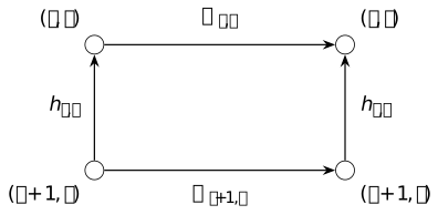
The temporal plaquette based at \((j,t)\) is traversed down the right edge, backwards along the bottom, up the left edge and then along the top. With the transport order, the first transport acts on the right and the product is exactly \(B_{j,e}\). Temporal averaging is retained at every step, so no periodic gauge-fixing assumption removes \(P\).
Example 33.6. Why the periodic trace needs gauge projection [fdip-0084]AGENTDRAFTED
- November 1, 2026
Example 33.6. Why the periodic trace needs gauge projection [fdip-0084]AGENTDRAFTED
- November 1, 2026
Take a graph with one edge and two distinct vertices, with \(G=\mathbb Z_2\), \(V=0\) and the sign kernel \(k(u)=e^{\beta u}\), \(\beta >0\). The link space has orthonormal basis \(1,u\), with \[T1=(\cosh \beta )1,\qquad Tu=(\sinh \beta )u.\] The two endpoint gauge transformations act by \(u\mapsto h_tuh_s\). Their action is transitive on the two link configurations. Thus the gauge projector satisfies \(P1=1\) and \(Pu=0\), and the physical space consists exactly of constants.
For every \(N\ge 1\), the projected and unprojected traces are \[\begin {aligned} \operatorname {Tr}(PT^N)&=(\cosh \beta )^N,\\ \operatorname {Tr}(T^N)&=(\cosh \beta )^N+(\sinh \beta )^N. \end {aligned}\] They are different because \(\beta >0\). In the temporal-link integral, each independent endpoint average gives \[\frac 14\sum _{h_s,h_t=\pm 1} e^{\beta U h_sU'h_t}=\cosh \beta .\] The remaining normalized link integrals contribute one, reproducing the projected answer. Dropping \(P\) would retain the nonphysical sign mode and change this finite periodic law.
Corollary 33.7. The physical spectral Hamiltonian [fdip-0085]AGENTDRAFTED
- November 1, 2026
Corollary 33.7. The physical spectral Hamiltonian [fdip-0085]AGENTDRAFTED
- November 1, 2026
For the physical transfer operator, let \(\lambda _0=\|T_{\mathrm {phys}}\|>0\) and fix a time step \(a_t>0\). There is an orthonormal eigenbasis \((\psi _j)\) with \(0<\lambda _j\le \lambda _0\), including an eigenvector at \(\lambda _0\). Define \[\widehat T=\frac {T_{\mathrm {phys}}}{\lambda _0},\qquad E_j=\frac 1{a_t}\log \frac {\lambda _0}{\lambda _j}.\] The transfer Hamiltonian is \(H=-a_t^{-1}\log \widehat T\), with the explicit domain and action \[\begin {aligned} D(H)&=\left \{f=\sum _jc_j\psi _j: \sum _jE_j^2|c_j|^2<\infty \right \},\\ Hf&=\sum _jE_jc_j\psi _j. \end {aligned}\] It is nonnegative and self-adjoint, and \(e^{-a_tH}=\widehat T\). If the physical Hilbert space is infinite dimensional, \(H\) is unbounded. This assertion does not specify the multiplicity of its zero eigenspace.
Proof.
- November 1, 2026
Proof.
- November 1, 2026
The spectral theorem for compact self-adjoint operators applies to the positive trace-class operator of Theorem 33.5. Injectivity removes its zero eigenspace, so the positive eigenvectors form a complete orthonormal basis. Its nonzero norm is an eigenvalue. In the finite-dimensional case the list is finite; otherwise its eigenvalues tend to zero.
The eigenspace-density assertion is formalized by
ContinuousLinearMap.orthogonalComplement_iSup_eigenspaces_eq_bot:
for a compact symmetric operator on a complete real or complex
inner-product space, the span of all eigenspaces has zero orthogonal
complement. This reference supplies that spectral premise; the
logarithm, its domain and its core are addressed below.
Under the unitary coefficient map \(f\mapsto (c_j)\), the normalized transfer is multiplication by \(\lambda _j/\lambda _0\). Its spectral logarithm is therefore multiplication by the real nonnegative sequence \(E_j\) on the stated maximal domain. This diagonal operator is self-adjoint; finite coefficient truncations form a core. Exponentiating on the basis proves the transfer identity. If the list is infinite, \(\lambda _j\to 0\) implies \(E_j\to \infty \), proving unboundedness.
This is the same normalization and domain construction as the Gaussian oscillator, without its explicit eigenvalues. It supplies a Hamiltonian at finite spatial volume. A unique vacuum, limits in time or volume, and a continuum field theory are separate questions, not conclusions of this spectral construction.
Theorem 33.8. Link reflection as a trace square [fdip-0086]AGENTDRAFTED
- November 1, 2026
Theorem 33.8. Link reflection as a trace square [fdip-0086]AGENTDRAFTED
- November 1, 2026
Use the periodic gauge law with \(N=2m\), \(m\ge 1\). Reflect time by \(\theta (j)=1-j\) modulo \(2m\); the positive half is \(\{1,\ldots ,m\}\). As in the scalar definition, this is a link reflection: its cuts lie between times \(0,1\) and \(m,m+1\).
Let \(\mathcal A_+\) consist of finite linear combinations of functions \[F(U)=\prod _{j=1}^m f_j(U_j),\] where each \(f_j:X\to \mathbb C\) is bounded, measurable and gauge invariant. These form an algebra of spatial observables. For such a product, on \(\mathcal H_{\mathrm {phys}}\) define \[A_F=T_{\mathrm {phys}}^{1/2}M_{f_1}T_{\mathrm {phys}} M_{f_2}\cdots T_{\mathrm {phys}}M_{f_m} T_{\mathrm {phys}}^{1/2},\] where for \(m=1\) this means \(T_{\mathrm {phys}}^{1/2}M_{f_1}T_{\mathrm {phys}}^{1/2}\). Extend this assignment linearly to finite sums. Then \(A_F\) is Hilbert–Schmidt and \[\mathbb E_{2m}\left [\overline {F(\theta U)}F(U)\right ] =\frac {\operatorname {Tr}(A_F^*A_F)}{Z_{2m}}\ge 0, \qquad (\theta U)_j=U_{1-j}.\] The temporal links have already been integrated in the periodic trace identity. No assertion about arbitrary observables involving individual temporal links is included.
Proof.
- November 1, 2026
Proof.
- November 1, 2026
The positive trace-class operator \(T_{\mathrm {phys}}\) has a Hilbert–Schmidt square root. Every multiplication operator here is bounded, as are all intervening transfer factors, so \(A_F\) is Hilbert–Schmidt; the same holds for a finite sum.
For products \(F=\prod _j f_j(U_j)\) and \(G=\prod _j g_j(U_j)\), the adjoint reverses the order and conjugates each multiplier. The bounded trace formula and cyclicity of a trace-class product give \[\operatorname {Tr}(A_F^*A_G) =Z_{2m}\,\mathbb E_{2m} \left [\overline {F(\theta U)}G(U)\right ].\] The cyclic order of the multipliers is \[\overline f_m,\ldots ,\overline f_1,g_1,\ldots ,g_m,\] with one full transfer between adjacent entries. They occur at times \(m+1,\ldots ,2m,1,\ldots ,m\), where \(2m=0\); hence \(f_j\) is conjugated at time \(1-j\). There are exactly \(2m\) transfer factors after the adjacent half-powers combine.
Expanding finite sums proves the same sesquilinear identity for all \(F,G\in \mathcal A_+\). If two product-sum presentations define the same function, their difference has zero expectation against its reflected conjugate, and the identity makes the corresponding difference of operators have Hilbert–Schmidt norm zero. Thus \(A_F\) is independent of that presentation. Taking \(G=F\) proves the trace-square identity and positivity.
This proof uses the explicitly positive operator of Theorem 33.4 and the exact finite-time law of Theorem 33.5. It does not reverse the argument to reconstruct a transfer operator from an arbitrary reflection-positive law; the scalar quotient obstruction shows why that distinction matters.
Remark 33.9. The scope of the finite gauge construction [fdip-0087]AGENTDRAFTED
- November 1, 2026
Remark 33.9. The scope of the finite gauge construction [fdip-0087]AGENTDRAFTED
- November 1, 2026
The positive convolution theorem and projected finite-time trace law concern a specified pure-gauge model on a finite spatial graph. Their assumptions are the strictly positive, summable character coefficients of Definition 33.1, not reflection positivity alone. The trace-square theorem applies to the stated algebra of bounded gauge-invariant spatial observables.
Lüscher's construction includes \(SU(N)\) gauge fields and Wilson fermions. Proposition 1 proves self-adjointness, boundedness, gauge invariance and strict positivity of its transfer operator. Its factorization and argument using tensor characters motivate the pure-gauge proof here. The fermion factors require the stated hopping assumptions, including \(0<K_{\mathrm {hop}}<1/6\); \(K_{\mathrm {hop}}\) is that paper's hopping parameter, not the spatial gauge group \(K\) used here. See [luscher1977transfer, pp. 286–288, Proposition 1].
Proposition 2 in [luscher1977transfer, p. 289] identifies time-ordered expectations under its specified gauge fixing and boundary conditions: periodic gauge fields and anticyclic fermions in time. The qualification on periodic temporal gauge appears in footnote 3 on p. 285. The direct projected integral of Theorem 33.5 retains temporal averaging, rather than using that gauge-fixing identification as a finite-periodic premise.
The spectral Hamiltonian has its stated maximal domain; boundedness of the transfer operator does not make its logarithm bounded. No unique-vacuum or continuum reconstruction claim is required. In particular, the joint Gaussian matter law and lattice fermion operators need their own transfer and positivity hypotheses.
34. Gauss's law and charged multiplicities [fdip-0088]AGENTDRAFTED
- November 1, 2026
34. Gauss's law and charged multiplicities [fdip-0088]AGENTDRAFTED
- November 1, 2026
The gauge transfer operator acts on all spatial link fields, while its physical trace uses gauge-invariant states. Temporal gauge explains the residual symmetry behind this constraint. With external charges, invariance applies to the link field together with its charge factors; it does not select a whole isotypic component of the link space.
The neutral projector is normalized averaging. Charged invariant tensors instead identify with a space of intertwiners. A single permutation-group link distinguishes a four-dimensional isotypic component from a one-dimensional charged space. A two-by-two sign lattice then counts neutral states by its gauge orbits. All graphs and time intervals here are finite.
Definition 34.1. Temporal gauge and the residual spatial action [fdip-0089]AGENTDRAFTED
- November 1, 2026
Definition 34.1. Temporal gauge and the residual spatial action [fdip-0089]AGENTDRAFTED
- November 1, 2026
Use the spatial graph and link space \(X=G^{E_s}\) and \(\mathcal H_{\mathrm {link}}=L^2(X,dU;\mathbb C)\). On a finite open time interval with slices \(0,\ldots ,N\), the temporal link \(h_{j,v}\) transports from \(j+1\) to \(j\) at spatial vertex \(v\). Allow independent gauge changes at all slices. For slice gauge changes \(g_j\in K\), where \(K=G^{V_s}\), it transforms as \[h_{j,v}\longmapsto g_{j,v}h_{j,v}g_{j+1,v}^{-1}.\] Temporal gauge means \(h_{j,v}=1\) on these temporal edges. Choose \(g_{0,v}\) and recursively set \(g_{j+1,v}=g_{j,v}h_{j,v}\) to reach this gauge.
A transformation preserving temporal gauge satisfies \(g_{j+1,v}=g_{j,v}\). Its remaining freedom is one spatial gauge transformation \(g\in K\), independent of time. This is the residual gauge action: \[(g\cdot U)_e=g_{t(e)}U_eg_{s(e)}^{-1},\qquad (R_gf)(U)=f(g^{-1}\cdot U).\] These are the same unitary operators used in the transfer construction, now interpreted on a time slice.
On a periodic time circle, the closure \(g_{N,v}=g_{0,v}\) changes the conclusion. The ordered temporal holonomy is \[H_v=h_{0,v}h_{1,v}\cdots h_{N-1,v}.\] The recursion closes exactly when \(H_v=1\). In general one can set the first \(N-1\) temporal links to one, but the last becomes \(g_{0,v}H_vg_{0,v}^{-1}\). Thus an arbitrary periodic field does not admit a gauge with every temporal link equal to one. The projected periodic trace keeps its temporal averaging and does not require such a gauge.
Kogut and Susskind's 1975 Hamiltonian formulation of Wilson's lattice gauge theories [kogut1975hamiltonian] provides historical context for this subject. The finite residual action above follows directly from the displayed transformation law; the state constraints below are established by averaging and representation theory.
Theorem 34.2. Neutral Gauss's law as an averaging constraint [fdip-008A]AGENTDRAFTED
- November 1, 2026
Theorem 34.2. Neutral Gauss's law as an averaging constraint [fdip-008A]AGENTDRAFTED
- November 1, 2026
For the residual action, the neutral Gauss constraint requires \[R_gf=f\qquad \text {for every }g\in K.\] Its solution space is the physical Hilbert space \(\mathcal H_{\mathrm {phys}}=\mathcal H_{\mathrm {link}}^K\). The orthogonal projector onto it is \[P=\int _KR_g\,dg,\] with normalized Haar measure. For a finite group \(G\), this is \[P=\frac 1{|G|^{|V_s|}}\sum _{g\in G^{V_s}}R_g.\] For the positive gauge transfer operator, \(TP=PT\); hence time evolution preserves the constraint.
Proof.
- November 1, 2026
Proof.
- November 1, 2026
For finite \(G\), left translation permutes the sum, so \(R_hPf=Pf\) for every \(h\). If \(f\) is invariant, every summand is \(f\), so \(Pf=f\). These facts prove \(P^2=P\) and identify its image. Unitarity gives \(R_g^*=R_{g^{-1}}\); inversion permutes the sum, proving \(P^*=P\). Thus \(P\) is the orthogonal projector.
For compact \(G\), the same identities use normalized Haar invariance, inversion and Fubini. The integral on \(L^2\), its boundedness and its image were proved in Theorem 33.5; that theorem applies here without a finite-group assumption. The transfer operator commutes with every \(R_g\) by Theorem 33.4, so it commutes with the average.
The finite algebraic projection statement is
Representation.isProj_averageMap. It assumes an
invertible group order in the coefficient ring, as holds over
\(\mathbb C\). Unitarity gives the orthogonality used here;
the compact Haar and transfer assertions have the separate proofs
just cited. Maschke averaging uses a related finite
average to produce invariant complements.
For a finite configuration set \(X\), an invariant function is exactly a function constant on each gauge orbit. Consequently \[\dim _{\mathbb C}\mathcal H_{\mathrm {phys}}=|X/K|.\] Indeed, the orbit indicators have disjoint support and form a basis. For Haar probability on a finite set, dividing each indicator by the square root of its orbit's probability makes this basis orthonormal.
Theorem 34.3. Charged invariant tensors and multiplicity spaces [fdip-008B]AGENTDRAFTED
- November 1, 2026
Theorem 34.3. Charged invariant tensors and multiplicity spaces [fdip-008B]AGENTDRAFTED
- November 1, 2026
Let \((R,\rho )\) be a specified finite-dimensional continuous unitary representation of the residual group \(K\) over \(\mathbb C\). Its complex linear dual \(R^*\) carries \((\rho ^*(g)\lambda )(v)=\lambda (\rho (g)^{-1}v)\). The charged physical space for this charge datum is \[\mathcal H_{\mathrm {phys}}(R) =(\mathcal H_{\mathrm {link}}\otimes R^*)^K,\] where \(g\) acts as \(R_g\otimes \rho ^*(g)\). Since \(R\) is finite dimensional, the Hilbert tensor product here is a finite orthogonal sum of copies of \(\mathcal H_{\mathrm {link}}\).
There is a canonical unitary identification \[\mathcal H_{\mathrm {phys}}(R) \cong \operatorname {Hom}_K(R,\mathcal H_{\mathrm {link}}) =:\mathcal M_R.\] Here \(\operatorname {Hom}_K\) consists of the linear maps \(F\) satisfying \(R_gF=F\rho (g)\) for every \(g\); its inner product is \(\langle F,G\rangle _{\mathrm {HS}}=\operatorname {Tr}(F^*G)\), linear in the second argument. The transfer operator \(T\otimes I\) preserves charged physical states and corresponds to \(F\mapsto TF\).
Suppose further that \(R\) is irreducible and put \(d=\dim R\). Its isotypic component in this complex Hilbert setting is \(\mathcal H_R\), defined as the closed span of all images \(F(R)\) with \(F\in \mathcal M_R\). Then \[\begin {aligned} R\otimes \mathcal M_R&\longrightarrow \mathcal H_R,\\ v\otimes F&\longmapsto \sqrt d\,F(v) \end {aligned}\] is a unitary representation isomorphism, with trivial \(K\)-action on \(\mathcal M_R\). The charged physical space is \(\mathcal M_R\), whereas \(\mathcal H_R\) includes the additional factor \(R\). In finite dimension, their dimensions are respectively \(\dim \mathcal M_R\) and \(d\dim \mathcal M_R\).
Proof.
- November 1, 2026
Proof.
- November 1, 2026
For an elementary tensor define \[\Phi (x\otimes \lambda )(v)=\lambda (v)x.\] If \(e_1,\ldots ,e_d\) is an orthonormal basis of \(R\) with dual basis \(e_1^*,\ldots ,e_d^*\), the inverse is \[F\longmapsto \sum _{i=1}^dF(e_i)\otimes e_i^*.\] Evaluating on the basis proves both inverse identities. The map \(\Phi \) is basis independent, so its inverse is as well. Its norm is the Hilbert–Schmidt norm \(\|F\|_{\mathrm {HS}}^2=\sum _i\|F(e_i)\|^2\), proving that \(\Phi \) is unitary.
Under \(\Phi \), the tensor action becomes \[F\longmapsto R_gF\rho (g)^{-1}.\] Indeed, apply both sides to \(v\) on an elementary tensor. Its fixed points are exactly the intertwiners, which proves the charged identification. The invariant subspace is closed, so \(\mathcal M_R\) is a Hilbert space. Since \(TR_g=R_gT\), postcomposition by \(T\) preserves intertwiners and corresponds to \(T\otimes I\).
For irreducible \(R\), unitarity and the intertwining identities show that \(F^*G:R\to R\) commutes with \(\rho (K)\). Complex Schur's lemma gives \[F^*G=\frac {\operatorname {Tr}(F^*G)}d I_R =\frac {\langle F,G\rangle _{\mathrm {HS}}}d I_R.\] One elementary proof of the lemma chooses an eigenvalue of a commuting complex endomorphism: its nonzero invariant eigenspace must be all of an irreducible representation. Therefore \[\langle F(v),G(w)\rangle =\frac 1d\langle v,w\rangle \langle F,G\rangle _{\mathrm {HS}}.\] Extending by linearity in finite sums proves that \(\sqrt d\) times evaluation is isometric. Its range is closed, and contains every \(F(R)\); by the definition of \(\mathcal H_R\), it is onto. The intertwining identity makes it equivariant. This proves the stated isotypic factorization and its normalization.
The algebraic tensor-to-map equivalence is formalized by
Representation.Equiv.dualTensorHom: its source order is
\(R^*\otimes \mathcal H_{\mathrm {link}}\), so first swap our two
factors. It requires finite-dimensional \(R\), with no dimension
restriction on \(\mathcal H_{\mathrm {link}}\).
The fixed-map step is formalized by
Representation.invariantsEquivIntertwiningMap for the
conjugation action on linear maps. The Hilbert–Schmidt isometry and
\(\sqrt d\) normalization are the direct arguments above. The earlier
real isotypic projectors and
multiplicity matrices concern whole representation
components; a projector onto such a component does not by itself
impose the charged tensor constraint.
For reducible charge data, first choose an irreducible orthogonal decomposition \(R=\bigoplus _\lambda R_\lambda \otimes \mathbb C^{n_\lambda }\). Applying the intertwiner identification to each summand gives \[\mathcal M_R\cong \bigoplus _\lambda \operatorname {Hom}(\mathbb C^{n_\lambda },\mathcal M_{R_\lambda }).\] This is an isomorphism of vector spaces. If all these spaces are finite dimensional and \(m_\lambda =\dim \mathcal M_{R_\lambda }\), then \(\dim \mathcal M_R=\sum _\lambda n_\lambda m_\lambda \). For the trivial one-dimensional charge, the construction recovers the neutral space.
Example 34.4. One permutation-group link has four isotypic states but one charged state [fdip-008C]AGENTDRAFTED
- November 1, 2026
Example 34.4. One permutation-group link has four isotypic states but one charged state [fdip-008C]AGENTDRAFTED
- November 1, 2026
Take one oriented edge with distinct source and target and \(G=S_3\). Then \(\mathcal H_{\mathrm {link}}=L^2(S_3)\) has complex dimension \(6\). Order the gauge factors as \(K=S_3^{\mathrm {target}}\times S_3^{\mathrm {source}}\); their function action is \[(R_{(h_t,h_s)}f)(U)=f(h_t^{-1}Uh_s).\] Let \(V=\{(z_1,z_2,z_3)\in \mathbb C^3:z_1+z_2+z_3=0\}\) carry the standard unitary permutation representation \(\rho \). Use the charge datum \[R=V_{\mathrm {target}}\otimes V_{\mathrm {source}}^*.\] It has dimension \(4\).
The standard representation is irreducible: a three-cycle has two distinct eigenlines on \(V\), with eigenvalues \(e^{2\pi i/3}\) and \(e^{-2\pi i/3}\), and a transposition exchanges them. Thus neither line is invariant under \(S_3\). The external tensor product \(R\) is also irreducible under \(K\). To see this, expand an endomorphism in a basis of \(\operatorname {End}(V^*)\). Commutation with the first factor and Schur's lemma make it \(I\otimes B\); commutation with the second factor makes \(B\) scalar. Any invariant subspace has a commuting orthogonal projector, so it is zero or all of \(R\).
The inverse matrix-coefficient map is \[\begin {aligned} \Psi :R&\longrightarrow L^2(S_3),\\ \Psi (v\otimes \lambda )(U) &=\sqrt 2\,\lambda (\rho (U^{-1})v). \end {aligned}\] Schur orthogonality makes this map isometric for normalized counting measure. Its order of duals is checked directly: \[R_{(h_t,h_s)}\Psi (v\otimes \lambda ) =\Psi (\rho (h_t)v\otimes \rho ^*(h_s)\lambda ).\] Thus its four-dimensional image is a copy of the specified charge representation, with the target and source conventions as stated.
The finite Peter–Weyl decomposition gives the bilateral decomposition \[L^2(S_3)\cong (\mathbf 1\otimes \mathbf 1) \oplus (\operatorname {sgn}\otimes \operatorname {sgn}) \oplus (V\otimes V^*).\] Indeed, the trivial, sign and standard representations are inequivalent, and their squared dimensions sum to \(1+1+4=6=|S_3|\), so their orthogonal coefficient spaces exhaust \(L^2(S_3)\). Hence the standard bilateral type has multiplicity one. By the charged-space theorem, \[\dim \mathcal H_R=4,\qquad \dim \mathcal H_{\mathrm {phys}}(R) =\dim \operatorname {Hom}_K(R,L^2(S_3))=1.\] The four-dimensional isotypic component is therefore not the charged physical space. Isotypic projectors separate representation types; invariant charge tensors supply the Gauss constraint.
Example 34.5. Thirty-two neutral states on a two-by-two sign torus [fdip-008D]AGENTDRAFTED
- November 1, 2026
Example 34.5. Thirty-two neutral states on a two-by-two sign torus [fdip-008D]AGENTDRAFTED
- November 1, 2026
Let the spatial vertices be \(V_s=(\mathbb Z/2\mathbb Z)^2\). For each vertex \(x\) and direction \(i\in \{1,2\}\), retain a separate edge \(e_{x,i}\) from \(x\) to \(x+\hat i\). There are 4 vertices and 8 indexed edges. In a period-two direction, \(e_{x,i}\) and \(e_{x+\hat i,i}\) have opposite endpoints but are distinct edges. The underlying graph is a multigraph with two parallel edges on each side of a square, not an ordinary four-cycle.
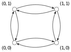
Each directed arc is one indexed edge. Horizontal and vertical arcs represent positive steps in the first and second coordinates, respectively; modulo two, both directions are positive coordinate steps. No face or plaquette constraint is imposed on the spatial link configurations in this example.
Take \(G=\mathbb Z_2\), written additively as \(\mathbb F_2\). A link configuration is \(u\in \mathbb F_2^{E_s}\), so \[\dim _{\mathbb C}\mathcal H_{\mathrm {link}}=2^8=256.\] A gauge function \(a\in \mathbb F_2^{V_s}\) acts by \[u_e\longmapsto u_e+a_{t(e)}+a_{s(e)}.\] The corresponding incidence map \(\delta :\mathbb F_2^{V_s}\to \mathbb F_2^{E_s}\) has kernel the constant functions: vanishing on every edge forces equal values along every path, and the graph is connected. Thus \(\dim \ker \delta =1\), \(\operatorname {rank}\delta =3\) and \(|\operatorname {im}\delta |=8\).
Every gauge orbit is a coset of \(\operatorname {im}\delta \), with 8 elements. The orbit basis therefore gives \[\dim _{\mathbb C}\mathcal H_{\mathrm {phys}} =\frac {256}{8}=32=2^5.\] The exponent is the cycle rank of this multigraph, \(b_1=|E_s|-|V_s|+1=8-4+1=5\). Equivalently, choose a spanning tree with three edges and set their additive link values to zero successively from a root. The remaining 5 chord values are free; the residual constant gauge function changes none of them. This supplies the same 32 representatives. The result counts neutral states of the link Hilbert space; it does not impose a flatness condition or identify opposite indexed edges.
35. Grassmann variables and finite fermion integrals [fdip-008E]AGENTDRAFTED
- November 1, 2026
35. Grassmann variables and finite fermion integrals [fdip-008E]AGENTDRAFTED
- November 1, 2026
Can electrons, which never share a state, be described in the probability-based setting? The spatial Dirac operator has a real matrix in its chosen basis and is skew-adjoint, so its real restriction satisfies \(D^T=-D\). For commuting real coordinates \(x\), transposition gives \(x^TDx=-x^TDx=0\). The weight \(e^{-x^TDx/2}\) is therefore constant, and adding a scalar mass leaves only \(m x^Tx\) in \(x^T(D+mI)x\): this quadratic expression loses the spatial operator.
Electrons are fermions: their multiparticle amplitudes change sign when two identical particles are exchanged [etingof2024mathematical, v2, Section 9.1, pp. 121-122]. Exclusion concerns the same complete one-particle state, including spin, not merely the same spatial orbital. The exterior algebra encodes the alternating sign through generators satisfying \(\psi _i\psi _j=-\psi _j\psi _i\) and \(\psi _i^2=0\) over \(\mathbb R\) or \(\mathbb C\). These are Grassmann variables. Their use here is an algebraic model of that sign rule, not a derivation of electron physics or a claim that measured fermion outcomes lack ordinary probabilities.
Integrating commuting Gaussian fields produces inverse powers of a determinant. For Grassmann variables, ordered top-coefficient extraction instead gives a determinant for independent paired variables and a Pfaffian for an alternating quadratic form. Two generators fix the signs before the general identities; the normalized Wick rule additionally requires invertibility. This algebraic integration is not a positive measure. Its relation to the earlier Clifford algebra is a vector-space comparison. Elimination, covariant lattice Dirac operators and their doubling problem are the later questions.
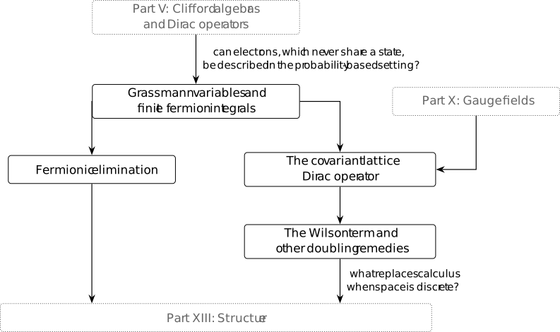
Definition 35.1. Ordered Berezin coefficients [fdip-008F]AGENTDRAFTED
- November 1, 2026
Definition 35.1. Ordered Berezin coefficients [fdip-008F]AGENTDRAFTED
- November 1, 2026
Let \(V\) be an \(N\)-dimensional vector space over \(\mathbb k=\mathbb R\) or \(\mathbb C\), with an ordered basis \(\xi _1,\ldots ,\xi _N\) of \(V^*\). The Grassmann algebra on these generators is the exterior algebra \(\Lambda (V^*)\). Multiplication is written by juxtaposition, so \[\xi _i\xi _j=-\xi _j\xi _i,\qquad \xi _i^2=0.\] Its basis consists of \(1\) and the increasing words \(\xi _{i_1}\cdots \xi _{i_r}\) with \(i_1<\cdots <i_r\); its dimension is \(2^N\). A word of length \(r\) has degree \(r\). Elements of even degree commute with every homogeneous element; two homogeneous elements of degrees \(r,s\) commute with sign \((-1)^{rs}\).
The Berezin integral with reversed top order is the linear functional \[I_\xi (f)=\text {coefficient of }\xi _N\cdots \xi _1 \text { in }f.\] Thus \(I_\xi (\xi _N\cdots \xi _1)=1\) and it vanishes on all lower degrees. Relative to the increasing top coefficient it has the sign \((-1)^{N(N-1)/2}\). For \(N=0\) it is the identity on \(\mathbb k\). This is the purely odd coefficient definition of [etingof2024mathematical, v2, Definition 9.6, p. 128], with the top order stated explicitly.
For \(n\) complex pairs, take \(2n\) independent generators \(\psi _1,\bar \psi _1,\ldots ,\psi _n,\bar \psi _n\) and use the paired functional \[J_n(f)=\text {coefficient of } \psi _1\bar \psi _1\cdots \psi _n\bar \psi _n \text { in }f.\] The bars label independent generators, not complex conjugates. The symbols \(I_\xi \) and \(J_n\) keep these two top-order conventions distinct. They are coefficient functionals, not positive measures on ordinary field configurations.
For a positive-degree nilpotent element \(q\), define
\(e^q=\sum _{r\ge 0}q^r/r!\); only finitely many terms survive.
For a quadratic \(q\) in \(N\) generators, terms with \(2r>N\)
vanish. No analytic convergence is involved. The ordered
monomial basis is supplied formally by
Module.Basis.ExteriorAlgebra; this supports the
algebraic coordinates, not the Berezin or Gaussian identities.
Example 35.2. Two generators fix the integration signs [fdip-008G]AGENTDRAFTED
- November 1, 2026
Example 35.2. Two generators fix the integration signs [fdip-008G]AGENTDRAFTED
- November 1, 2026
Take two generators and the alternating matrix \[A=\begin {pmatrix}0&a\\-a&0\end {pmatrix}.\] Anticommutation gives \[\tfrac 12\xi ^TA\xi =a\xi _1\xi _2.\] Since \((\xi _1\xi _2)^2=0\), \[e^{-\frac 12\xi ^TA\xi } =1-a\xi _1\xi _2=1+a\xi _2\xi _1.\] The reversed coefficient therefore gives \(I_\xi (e^{-\xi ^TA\xi/2})=a\). Selecting the increasing word \(\xi _1\xi _2\) instead would give \(-a\).
For one independent complex pair and any \(k\in \mathbb C\), \[e^{-k\bar \psi \psi }=1-k\bar \psi \psi =1+k\psi \bar \psi ,\qquad J_1(e^{-k\bar \psi \psi })=k.\] Both calculations use only the finite expansion and the ordered functionals in the definition, including when \(a=0\) or \(k=0\).
Theorem 35.3. Paired Grassmann integration gives a determinant [fdip-008H]AGENTDRAFTED
- November 1, 2026
Theorem 35.3. Paired Grassmann integration gives a determinant [fdip-008H]AGENTDRAFTED
- November 1, 2026
For any complex \(n\times n\) matrix \(K\), use the independent generators and paired top order. Then \[J_n\left (e^{-\bar \psi K\psi }\right )=\det K, \qquad \bar \psi K\psi =\sum _{i,j=1}^n\bar \psi _iK_{ij}\psi _j.\] No invertibility or positivity assumption is needed. The empty case has \(J_0(1)=1\), equal to the determinant of the empty matrix.
Proof.
- November 1, 2026
Proof.
- November 1, 2026
Move each barred generator to the right and put \[q_i=\sum _{j=1}^nK_{ij}\psi _j\bar \psi _i, \qquad -\bar \psi K\psi =\sum _iq_i.\] Each \(q_i^2=0\), because every term repeats \(\bar \psi _i\). The \(q_i\) have even degree and commute, so finite expansion gives \[e^{\sum _iq_i}=\prod _{i=1}^n(1+q_i).\] Only \(q_1\cdots q_n\) can contribute to the top degree. A nonzero term in that product chooses every unbarred generator once, hence is indexed by a permutation \(\sigma \in S_n\).
The associated word is \(\psi _{\sigma (1)}\bar \psi _1\cdots \psi _{\sigma (n)}\bar \psi _n\). Moving all barred factors to the right gives \((-1)^{n(n-1)/2}\). Sorting the unbarred factors gives \(\operatorname {sgn}(\sigma )\). Returning the bars to the paired top order gives the same first sign again. Their product is \(\operatorname {sgn}(\sigma )\). Thus the required coefficient is \[\sum _{\sigma \in S_n}\operatorname {sgn}(\sigma ) \prod _{i=1}^nK_{i,\sigma (i)}=\det K.\]
Selecting the grouped top word \(\psi _1\cdots \psi _n\bar \psi _1\cdots \bar \psi _n\) would instead give \((-1)^{n(n-1)/2}\det K\). There is a local ordering discrepancy in [etingof2024mathematical, v2, Proposition 9.10, p. 131]: the volume displayed immediately before the proposition is interleaved, whereas its printed determinant sign is the grouped one under Definition 9.6's coefficient rule. For \(n=2,K=I\), the exponential is \((1+\psi _1\bar \psi _1)(1+\psi _2\bar \psi _2)\); its interleaved coefficient is \(+1\) and its grouped coefficient is \(-1\). The direct expansion above fixes the convention used here.
Definition 35.4. The Pfaffian records signed pairings [fdip-008I]AGENTDRAFTED
- November 1, 2026
Definition 35.4. The Pfaffian records signed pairings [fdip-008I]AGENTDRAFTED
- November 1, 2026
Let \(A^T=-A\) be a \(2m\times 2m\) matrix over \(\mathbb R\) or \(\mathbb C\). A perfect matching of \(\{1,\ldots ,2m\}\) partitions it into pairs \((i_1,j_1),\ldots ,(i_m,j_m)\), written with \(i_r<j_r\) and \(i_1<\cdots <i_m\). Let \(\varepsilon (M)\) be the sign of the permutation with word \(i_1,j_1,\ldots ,i_m,j_m\). The Pfaffian is \[\operatorname {Pf}(A) =\sum _M\varepsilon (M)\prod _{r=1}^m A_{i_rj_r}.\] The empty Pfaffian is \(1\). This is the matching formula in [etingof2024mathematical, v2, Section 9.9, pp. 130-131].
Grouping matchings by the partner \(j\) of \(1\) gives \[\operatorname {Pf}(A)= \sum _{j=2}^{2m}(-1)^j A_{1j} \operatorname {Pf}(A_{\widehat 1\widehat j}),\] where the indicated two rows and columns are deleted, retaining the original order. Indeed, moving \(j\) immediately after \(1\) crosses \(j-2\) entries. In dimensions two and 4 this reads \[\operatorname {Pf}\begin {pmatrix}0&a\\-a&0\end {pmatrix}=a,\] \[\operatorname {Pf}(A)=A_{12}A_{34}-A_{13}A_{24}+A_{14}A_{23}.\] Each term pairs every index exactly once; unlike a determinant expansion, it sums over pairings rather than all permutations.
Theorem 35.5. An odd quadratic integral is a Pfaffian [fdip-008J]AGENTDRAFTED
- November 1, 2026
Theorem 35.5. An odd quadratic integral is a Pfaffian [fdip-008J]AGENTDRAFTED
- November 1, 2026
Let \(A^T=-A\) on \(2m\) generators and use the reversed top coefficient. Then \[I_\xi \left (e^{-\frac 12\xi ^TA\xi }\right ) =\operatorname {Pf}(A).\] This holds for singular as well as invertible \(A\). If \(A\) is invertible, then \(\operatorname {Pf}(A)\ne 0\).
Proof.
- November 1, 2026
Proof.
- November 1, 2026
Put \(\Omega =\sum _{i<j}A_{ij}\xi _i\xi _j =\xi ^TA\xi/2\). In \(\Omega ^m\), a nonzero top word uses each generator exactly once. The even two-letter factors commute; every matching appears in \(m!\) orders. Reordering its word to \(\xi _1\cdots \xi _{2m}\) gives its matching sign. Therefore \[\frac {\Omega ^m}{m!} =\operatorname {Pf}(A)\xi _1\cdots \xi _{2m}.\] The top term of \(e^{-\Omega }\) is \((-1)^m\Omega ^m/m!\). Reversing \(2m\) generators has sign \((-1)^{m(2m-1)}=(-1)^m\); the two signs cancel. This proves the integral identity, without an inverse.
For the nonvanishing assertion, regard \(A\) as a nondegenerate alternating form on the vector space dual to the generators. Choose a nonzero \(u\) and then \(v\) with \(A(u,v)=1\). The plane they span is nondegenerate, and its orthogonal complement for \(A\) is a direct complement on which \(A\) remains nondegenerate. Induction gives a basis of such pairs. In the dual basis \(\alpha _1,\beta _1,\ldots ,\alpha _m,\beta _m\), \[\Omega =\sum _{r=1}^m\alpha _r\beta _r,\qquad \frac {\Omega ^m}{m!}=\alpha _1\beta _1\cdots \alpha _m\beta _m\ne 0.\] An invertible change of generators multiplies a top word by a nonzero determinant. The displayed top coefficient is therefore nonzero in the original basis as well, proving \(\operatorname {Pf}(A)\ne 0\). The zero-dimensional case is \(1\).
In [etingof2024mathematical, v2, Proposition 9.9, p. 131], the increasing top order accompanies a positive quadratic exponent. Replacing \(A\) by \(-A\) contributes \((-1)^m\) to the Pfaffian, and reversing the top order contributes the same sign. Thus the convention conversion agrees with the direct proof.
Theorem 35.6. The odd Wick rule pairs inverse alternating entries [fdip-008K]AGENTDRAFTED
- November 1, 2026
Theorem 35.6. The odd Wick rule pairs inverse alternating entries [fdip-008K]AGENTDRAFTED
- November 1, 2026
Let \(A^T=-A\) be an invertible \(2m\times 2m\) matrix. Its nonzero Pfaffian defines the normalized linear functional \[W_A(f)=\frac {I_\xi (f e^{-\xi ^TA\xi/2})} {\operatorname {Pf}(A)}.\] For linear Grassmann elements \(\lambda _a=\sum _i\ell _{ai}\xi _i\), put \(C_{ab}=\ell _aA^{-1}\ell _b^T\). For every \(r\ge 0\), \[W_A(\lambda _1\cdots \lambda _{2r})=\operatorname {Pf}(C),\] where \(C\) is the \(2r\times 2r\) alternating matrix just defined. Every odd product has value zero. Repeated or dependent \(\lambda _a\) are allowed. The inverse formula requires invertible \(A\); it asserts no singular extension.
Proof.
- November 1, 2026
Proof.
- November 1, 2026
Define the left derivative on a monomial by \[\partial _i(\xi _{j_1}\cdots \xi _{j_s}) =\sum _{a=1}^s(-1)^{a-1}\delta _{i,j_a} \xi _{j_1}\cdots \widehat {\xi _{j_a}}\cdots \xi _{j_s}.\] This respects the exterior relations. Splitting the removed positions between two factors gives the graded product rule \[\partial _i(fg)=(\partial _i f)g+(-1)^s f(\partial _i g)\] when \(f\) is homogeneous of degree \(s\). It lowers degree, so \(I_\xi (\partial _i h)=0\) for every \(h\).
Write \(E=e^{-\xi ^TA\xi/2}\). Differentiating its finite series, using that its quadratic exponent is even, gives \[\partial _iE=-\sum _jA_{ij}\xi _jE.\] For odd homogeneous \(f\), the product rule and coefficient of the total derivative imply \[\begin {aligned} 0&=I_\xi ((\partial _i f)E+f\sum _jA_{ij}\xi _jE),\\ \sum _jA_{ij}W_A(\xi _jf)&=W_A(\partial _i f). \end {aligned}\] The second line uses \(f\xi _j=-\xi _jf\). Multiplying by \(A^{-1}\) gives \[W_A(\xi _kf)=\sum _i(A^{-1})_{ki}W_A(\partial _i f).\]
Apply this to \(f=\lambda _2\cdots \lambda _{2r}\) and expand \(\lambda _1\). The derivative removes its \(a\)-th listed factor with sign \((-1)^{a-2}\), yielding \[\begin {aligned} W_A(\lambda _1\cdots \lambda _{2r}) &=\sum _{a=2}^{2r}(-1)^a C_{1a}\\ &\quad \cdot W_A(\lambda _2\cdots \widehat {\lambda _a} \cdots \lambda _{2r}). \end {aligned}\] Starting from \(W_A(1)=1\), this is exactly the Pfaffian recursion. Odd products have odd degree, while \(E\) has only even degrees and the selected top degree \(2m\) is even; hence their integrals vanish.
The left derivative is contraction by the coordinate functional
\(\xi _j\mapsto \delta _{ij}\). TauCeti's
TauCeti.ExteriorAlgebra.contractLeft_ιMulti
gives the alternating deletion formula. At zero quadratic form,
CliffordAlgebra.contractLeft_mul
gives the product rule: the grade involution acts by \((-1)^s\)
in degree \(s\). These support the contraction identities;
the Berezin normalization and Wick recurrence are the direct
argument above.
For \(A=\left (\begin {smallmatrix}0&a\\-a&0\end {smallmatrix}\right )\) with \(a\ne 0\), the two-generator calculation gives \(W_A(\xi _1\xi _2)=-1/a=(A^{-1})_{12}\). This checks the inverse-pairing sign. In [etingof2024mathematical, v2, Theorem 9.11, p. 132], the increasing top order gives normalization \(\operatorname {Pf}(-A)\). Changing the volume multiplies both numerator and normalization by the same sign, leaving this normalized Wick rule unchanged.
Remark 35.7. Exterior symbols preserve vectors, not Clifford products [fdip-008L]AGENTDRAFTED
- November 1, 2026
Remark 35.7. Exterior symbols preserve vectors, not Clifford products [fdip-008L]AGENTDRAFTED
- November 1, 2026
The Grassmann algebra and the earlier
configuration Clifford algebra share an exterior
vector-space model. For a quadratic form \(q\) on \(V^*\),
the symbol map is a linear isomorphism
\[\operatorname {Cl}(V^*,q)\cong \Lambda (V^*).\]
This is [meinrenken2013clifford, Proposition 2.5, pp. 32-33]
and the equivalence used in the
transported exterior-basis coordinates.
The formal declaration CliffordAlgebra.equivExterior
supplies a module equivalence over any commutative ring in which
\(2\) is invertible; it does not identify the products.
For example, an exterior generator satisfies \(\xi ^2=0\), while the corresponding Clifford generator satisfies \(\iota _q(\xi )^2=q(\xi )1\). For \(q(\xi )\ne 0\) these cannot be the same multiplication under a unit-preserving map. The quadratic form remains in Clifford contraction terms. The associated graded algebra forgets those lower terms, but the Clifford algebra itself does not. Therefore the Berezin functional and its determinant formulas belong to the exterior product; the vector-space comparison alone does not transfer them to a Clifford product.
36. Fermionic elimination [fdip-009I]AGENTDRAFTED
- November 1, 2026
36. Fermionic elimination [fdip-009I]AGENTDRAFTED
- November 1, 2026
What remains after some fermion variables are eliminated? The paired Grassmann integral replaces a Gaussian normalizer by a determinant, but the effective quadratic form is still a Schur complement. The eliminated block must be invertible; the full matrix need not be positive or invertible for this algebraic identity.
A commuting complex field supplies the inverse determinant when the Hermitian part of its matrix is positive. This is an ordinary convergent integral on twice as many real coordinates. Its cancellation with the Grassmann determinant uses the same matrix in both quadratic forms. A non-Hermitian accretive matrix usually gives a complex weight, so this cancellation does not construct a positive joint probability law.
The logarithm of the determinant needs an additional choice. On the accretive cone there is a unique analytic logarithm normalized at the identity; it need not be the principal scalar logarithm of the determinant. The four-cycle makes these distinctions concrete with the same effective matrix as in real Gaussian elimination.
Theorem 36.1. Partial Grassmann integration and the Schur complement [fdip-009J]AGENTDRAFTED
- November 1, 2026
Theorem 36.1. Partial Grassmann integration and the Schur complement [fdip-009J]AGENTDRAFTED
- November 1, 2026
Let \(R,U\) be disjoint ordered finite sets. Order the independent paired generators with all retained \(R\)-pairs first and all eliminated \(U\)-pairs second. For \(n=|R|+|U|\), let \[K=\begin {pmatrix}A&B\\C&D\end {pmatrix} \in M_n(\mathbb C).\] Require \(D=K_{UU}\) to be invertible and put \(S=A-BD^{-1}C\). No adjoint relation between \(B,C\) is assumed. Define \(J_U\) by taking the coefficient of the ordered \(U\)-pair top word after moving retained generators to the left. The result is an element of the retained exterior algebra. Define \(J_R\) by its paired top word, so \(J_RJ_U=J_n\). The eliminated top word has even degree, so moving it past a retained coefficient gives no further sign. Then \[J_U\left (e^{-\bar \psi K\psi }\right ) =\det D\,e^{-\bar \psi _R S\psi _R},\] and consequently \[\det K=\det D\det S.\] The empty-block conventions are determinant one and the identity coefficient map. Invertibility of \(K\) or \(S\) is unnecessary.
Proof.
- November 1, 2026
Proof.
- November 1, 2026
Introduce the odd linear combinations \[\begin {aligned} \chi _U&=\psi _U+D^{-1}C\psi _R,\\ \bar \chi _U&=\bar \psi _U+\bar \psi _RBD^{-1}. \end {aligned}\] The bars remain labels of independent generators. Expanding in the displayed multiplication order gives \[\bar \psi K\psi =\bar \psi _R S\psi _R+\bar \chi _U D\chi _U.\] For example, the last term of the expansion of \(\bar \chi _U D\chi _U\) is \(\bar \psi _RBD^{-1}C\psi _R\), which cancels the subtraction in \(S\). All these quadratic elements are even. They commute, so their finite exponentials multiply.
Replacing an eliminated generator by itself plus a retained odd linear combination preserves its partial top coefficient. Indeed, expand each exterior monomial in the new symbols: every term using a retained replacement has fewer eliminated generators, while the term using no replacement has coefficient one and its original order. Terms of lower eliminated degree cannot contribute to the top degree. Thus the coefficient in the shifted quadratic exponential equals the coefficient for independent \(U\)-generators. The paired determinant identity evaluates it as \(\det D\). The retained exponential factors on the left, proving the partial formula. Applying \(J_R\) and the same determinant identity proves the full factorization.
The effective matrix is the same block expression as in real positive Gaussian elimination. The scalar here is \(\det D\); the real Gaussian fiber integral instead has \((2\pi )^{|U|/2}(\det D)^{-1/2}\) under its real positive hypotheses and volume convention. Neither positivity nor an ordinary integration measure was used in the Grassmann proof.
The finite block identity is also supplied by
Matrix.det_fromBlocks₂₂, for finite index types over a
commutative ring with an invertible eliminated block. This
formal statement supports the determinant factorization, not
the partial Grassmann coefficient operation.
Theorem 36.2. Accretive complex Gaussian integrals and cancellation [fdip-009K]AGENTDRAFTED
- November 1, 2026
Theorem 36.2. Accretive complex Gaussian integrals and cancellation [fdip-009K]AGENTDRAFTED
- November 1, 2026
Call \(K\in M_n(\mathbb C)\) strictly accretive when its Hermitian part \(H=(K+K^*)/2\) is positive definite. For \(z_j=x_j+iy_j\), use ordinary Lebesgue volume \(d^{2n}z=\prod _j dx_j\,dy_j\). Then \(K\) is invertible, the following integral converges absolutely, and \[I(K):=\int _{\mathbb C^n}e^{-z^*Kz}\,d^{2n}z =\frac {\pi ^n}{\det K}.\] Consequently, with \(Z_B(K)=\pi ^{-n}I(K)\) and the paired Grassmann value \(Z_F(K)=J_n(e^{-\bar \psi K\psi })\), \[Z_B(K)Z_F(K)=1.\] For \(n=0\) both factors are one.
Proof.
- November 1, 2026
Proof.
- November 1, 2026
For \(n>0\), choose \(h>0\) with \(H\ge hI\). Then \[|e^{-z^*Kz}|=e^{-z^*Hz}\le e^{-h\|z\|^2}.\] The right side is integrable by the product of scalar Gaussian integrals. If \(Kz=0\), its real quadratic value is \(z^*Hz=0\), so \(z=0\); finite dimension makes \(K\) invertible.
First suppose \(K=K^*>0\). A unitary eigenbasis gives positive eigenvalues \(\lambda _j\). The unitary change of variables preserves real volume, since its real Jacobian has absolute determinant \(|\det _{\mathbb C}U|^2=1\). In each complex coordinate the scalar Gaussian formula gives \[\int _{\mathbb R^2}e^{-\lambda _j(x^2+y^2)}dx\,dy =\frac \pi {\lambda _j}.\] Multiplication gives \(I(K)=\pi ^n/\det K\).
For general \(K\), write \(K=H+A\), where \(A^*=-A\), and set \(K(w)=H+wA\) for a complex parameter \(w\). Its Hermitian part is \(H+i(\operatorname {Im}w)A\). Choose \(\epsilon >0\) such that \(\epsilon \|A\|<h/2\), with any positive choice if \(A=0\). On the connected strip \(|\operatorname {Im}w|<\epsilon \), this part is at least \(hI/2\), so \(K(w)\) is invertible.
The integral \(I(K(w))\) is holomorphic on that strip. Differentiation of the integrand brings down powers of \(-z^*Az\); on every smaller neighborhood these are bounded by a polynomial in \(\|z\|\) times \(e^{-h\|z\|^2/2}\). This integrable bound justifies differentiation under the integral. The function \(\pi ^n/\det K(w)\) is holomorphic there too. For \(w=it\) with real \(|t|<\epsilon \), the matrix \(H+itA\) is Hermitian positive, so the preceding calculation identifies the two functions. These points accumulate at the interior point zero. The one-variable identity theorem therefore identifies the functions throughout the strip, in particular at \(w=1\). The Grassmann determinant then proves cancellation.
For Hermitian positive \(K\), the normalized density \((\det K/\pi ^n)e^{-z^*Kz}\) is a genuine Gaussian probability law on \(2n\) real coordinates. For general accretive \(K\), the weight can be complex: \(K=(1+i)\) gives \(Z_F=1+i\) and \(Z_B=(1+i)^{-1}\). Normalization and determinant cancellation still hold, but there is no positive Gaussian law with this density. A single real Gaussian has only a determinant power \(-1/2\); Grassmann algebra by itself supplies no convergence for a commuting integral.
Accretivity also survives the Schur operation. Its principal block \(D\) is accretive by testing \(K\) on \((0,u)\), hence invertible. For \(v\ne 0\), put \(x=(v,-D^{-1}Cv)\). Then \(Kx=(Sv,0)\), and \[\operatorname {Re}(v^*Sv) =\operatorname {Re}(x^*Kx)>0.\] Thus \(S\) is accretive. This extra conclusion uses accretivity of the full matrix, not just invertibility of \(D\).
[wingate2025lattice, Section 9.1, equations (9.3)-(9.5), p. 19] describes integrating a fermion matrix and re-expressing its determinant with commuting complex pseudofermions. Its equation (9.5) uses \(K^{-1}\) in the commuting quadratic form, yielding a determinant rather than its inverse when convergence holds. The cancellation here uses \(K\) in both forms and the specified factor \(\pi ^{-n}\); the proof above states its convergence hypotheses explicitly.
Proposition 36.3. The logarithm on the accretive cone [fdip-009L]AGENTDRAFTED
- November 1, 2026
Proposition 36.3. The logarithm on the accretive cone [fdip-009L]AGENTDRAFTED
- November 1, 2026
On the open convex cone \(\mathcal C_n\) of strictly accretive complex matrices, there is a unique holomorphic function \(\mathcal L\) such that \[e^{\mathcal L(K)}=\det K,\qquad \mathcal L(I)=0.\] For \(K_t=I+t(K-I)\), it is given by \[\mathcal L(K)=\int _0^1 \operatorname {tr}\left [K_t^{-1}(K-I)\right ]dt.\] On Hermitian positive matrices it equals the real \(\log \det K\). Thus the fermionic logarithmic contribution \(W_F(K)=-\mathcal L(K)\) is unambiguous on this cone.
Proof.
- November 1, 2026
Proof.
- November 1, 2026
Write \(K_t=I+t(K-I)\). Convexity makes \(K_t\) accretive and invertible for every \(0\le t\le 1\). In a neighborhood of each \(K\in \mathcal C_n\), the Hermitian parts of all these matrices have a common positive lower bound. Their inverses and derivatives in the matrix entries are therefore locally bounded uniformly in \(t\). The integral of the holomorphic rational integrand is holomorphic in \(K\).
Put \(g(t)=\det K_t\). The determinant derivative, as in the real log-determinant calculation, gives \[\frac {g'(t)}{g(t)} =\operatorname {tr}(K_t^{-1}(K-I)).\] This complex version follows directly from \(\det (K_t+hB)=\det K_t\det (I+hK_t^{-1}B)\) and \(\det (I+hM)=1+h\operatorname {tr}M+O(h^2)\), obtained by the permutation expansion. Therefore the derivative of \(g(t)\exp (-\int _0^t g'(s)/g(s)\,ds)\) is zero. Its value at zero is one, proving \(\exp \mathcal L(K)=\det K\); the identity matrix gives \(\mathcal L(I)=0\).
Two such logarithms differ by a continuous function with values in \(2\pi i\mathbb Z\). The cone is connected, so this function is constant, and normalization makes it zero. On Hermitian positive \(K\), all \(K_t\) are positive and \(g(t)>0\); ordinary real logarithmic differentiation identifies the integral with \(\log \det K\).
This branch is not always the principal scalar logarithm of \(\det K\). For \(K=e^{i\pi /3}I_4\), the Hermitian part is \(I_4/2>0\). Along \(K(s)=e^{is}I_4\), \(0\le s\le \pi /3\), continuity and normalization give \(\mathcal L(K(s))=4is\). Hence \[\mathcal L(e^{i\pi /3}I_4)=\frac {4\pi i}{3},\] whereas the principal scalar logarithm of its determinant is \(-2\pi i/3\). The determinant can even reach the scalar principal branch cut while the matrix stays accretive.
For a general invertible complex matrix, writing \(-\log \det K\) requires a declared branch on the domain under consideration; there is no single-valued continuous logarithm on all invertible matrices when \(n\ge 1\). The loop \(\operatorname {diag}(e^{it},1,\ldots ,1)\), \(0\le t\le 2\pi \), already has determinant winding once. If \(\det K=0\), no logarithm exists, although the Grassmann determinant identity still does. The boson-fermion cancellation itself uses no logarithm branch.
Example 36.4. The same four-cycle Schur matrix with fermions [fdip-009M]AGENTDRAFTED
- November 1, 2026
Example 36.4. The same four-cycle Schur matrix with fermions [fdip-009M]AGENTDRAFTED
- November 1, 2026
Take the alternating four-cycle with \(t,m>0\), set \(a=m^2\), \(s=1+t+a\), and use \(K=Q_{t,m}=L_t+aI\) now as a complex matrix. Order retained vertices \(R=(0,2)\) before eliminated vertices \(U=(1,3)\). Its blocks are \[A=D=sI_2,\qquad B=C=-\begin {pmatrix}1&t\\t&1\end {pmatrix}.\] The fermionic Schur formula gives \[J_U(e^{-\bar \psi K\psi }) =s^2e^{-\bar \psi _R S\psi _R},\] where \[\begin {aligned} S&=\begin {pmatrix}\alpha &-\beta \\-\beta &\alpha \end {pmatrix},\\ \alpha &=s-\frac {1+t^2}{s},\qquad \beta =\frac {2t}{s}. \end {aligned}\] This is exactly the real Gaussian effective precision. The fermionic scalar is \(s^2\); the real Gaussian eliminated factor in the cited example is \(2\pi /s\).
The two eigenvalues of \(S\) are \[\frac {a(a+2+2t)}s,\qquad \frac {(a+2)(a+2t)}s.\] Writing \(\mathcal D=a(a+2)(a+2t)(a+2+2t)\), it follows that \[\det S=\frac {\mathcal D}{s^2},\qquad Z_F(K)=s^2\det S=\mathcal D.\] Positivity of \(K\) also allows the ordinary complex integral with normalized volume \(\pi ^{-4}d^8z\). The complex Gaussian theorem gives \[Z_B(K)=\mathcal D^{-1},\qquad Z_F(K)Z_B(K)=1.\] In contrast, the original real Gaussian, with exponent \(-\phi ^TK\phi /2\) and volume \(d^4\phi \), has partition function \((2\pi )^2/\sqrt {\mathcal D}\). These powers and constants refer to different field spaces and measures.
At \(t=m=1\), \(s=3\), \(\mathcal D=45\), and \[S=\begin {pmatrix}7/3&-2/3\\-2/3&7/3\end {pmatrix}, \qquad \det S=5.\] The Grassmann eliminated factor \(9\) times the retained factor \(5\) gives \(45\), while the normalized complex-boson value is \(1/45\). At \(t=2,m=1\), \(s=4\), \(\det S=105/16\); the product is \(16\cdot 105/16=105\). These are the same two effective matrices compared in the weighted-cycle example.
At \(m=0,t>0\), the eliminated block \((1+t)I_2\) is still invertible and the partial Grassmann formula is valid. The retained Schur matrix has a constant zero mode, so \(\det K=0\): the full Grassmann integral vanishes. The commuting full Gaussian instead diverges in its constant mode. There is no finite inverse determinant, cancellation identity or logarithmic contribution at this massless point.
37. The covariant lattice Dirac operator [fdip-009N]AGENTDRAFTED
- November 1, 2026
37. The covariant lattice Dirac operator [fdip-009N]AGENTDRAFTED
- November 1, 2026
How does a fermion move through a fixed gauge connection? The spatial Dirac operator combines centered differences with Clifford matrices. The connection background compares fields at neighboring vertices by parallel transport. Combining them requires two separate factors: a Clifford module \(S\) and an internal representation \(F\). The gauge links act on \(F\), while the gamma matrices act on \(S\).
This separation makes the operator gauge covariant and skew-adjoint. It also identifies its finite matrix as a possible kernel for the paired Grassmann integral, without claiming a positive probability density. At the trivial connection, the Fourier blocks retain the centered difference's sine symbol. Their exact zero modes depend on the parity of the finite periods; the extra local branches of the continuous momentum symbol are a different count. Fixed antiperiodic boundary conditions change the sampling but do not remove those branches.
A group acting on spin frames has a different role from an internal gauge group. Even when both are described using \(SU(2)\) or a binary rotation group, their actions and the Clifford compatibility must be supplied separately.
Definition 37.1. Covariant centered differences with an internal fiber [fdip-009O]AGENTDRAFTED
- November 1, 2026
Definition 37.1. Covariant centered differences with an internal fiber [fdip-009O]AGENTDRAFTED
- November 1, 2026
Use the periodic grid and Clifford module: \(d\ge 1\), periods \(N_j\ge 3\), \(\Lambda =\prod _j\mathbb Z/N_j\mathbb Z\), and \(S=(\mathbb C^2)^{\otimes d}\) with Hermitian matrices \(\gamma _j\). Thus \(\dim _{\mathbb C}S=2^d\) and \[\gamma _i\gamma _j+\gamma _j\gamma _i=2\delta _{ij}I_S.\] The lattice spacing is one. Choose a nonzero finite-dimensional complex Hermitian space \(F\), with \(q=\dim _{\mathbb C}F\), and a unitary representation \(\rho :G\to U(F)\) of a finite or compact group, continuous in the compact case. The invariant metric is part of the representation datum. The field space is \[\mathcal H=\ell ^2(\Lambda )\otimes S\otimes F,\] identified with maps \(\psi :\Lambda \to S\otimes F\), with \[\langle \psi ,\phi \rangle =\sum _{x\in \Lambda }\langle \psi (x),\phi (x)\rangle _{S\otimes F}.\] Dimensions are over \(\mathbb C\); adjoints use the declared Hermitian inner products.
Assign \(U_j(x)\in G\) to the oriented edge \(x\to x+e_j\), and also write \(U_j(x)\) for its unitary action \(\rho (U_j(x))\) on \(F\). The source-to-head convention means that comparing a value at \(x+e_j\) with one at \(x\) uses the inverse transport. Define \[\begin {gathered} (T_j^U\psi )(x) = (I_S\otimes U_j(x)^{-1})\psi (x+e_j),\\ ((T_j^U)^{-1}\psi )(x)\\ = (I_S\otimes U_j(x-e_j))\psi (x-e_j). \end {gathered}\] Substitution verifies that the second operator is the inverse of the first. Put \[\nabla _j^U=\frac {T_j^U-(T_j^U)^{-1}}2,\qquad \Gamma _j=\gamma _j\otimes I_F,\] where \(\Gamma _j\) acts pointwise on the field. The covariant lattice Dirac operator is \[D_U=\sum _{j=1}^d\Gamma _j\nabla _j^U.\] This is the centered nearest-neighbor convention in [wingate2025lattice, Section 9.1, Equations (9.1)–(9.2), p. 19], with spacing one and the declared link orientation.
For \(g:\Lambda \to G\), write \(g_x=\rho (g(x))\) in operator formulas. The transformed links and field are \[\begin {aligned} U_j^g(x)&=g_{x+e_j}U_j(x)g_x^{-1},\\ (\mathcal G\psi )(x)&=(I_S\otimes g_x)\psi (x). \end {aligned}\] This is an internal gauge transformation: it fixes the lattice and the chosen Clifford matrices. Links and \(\mathcal G\) commute with every \(\Gamma _j\), because they act on the other tensor factor.
Theorem 37.2. Gauge covariance and skew-adjointness of the Dirac operator [fdip-009P]AGENTDRAFTED
- November 1, 2026
Theorem 37.2. Gauge covariance and skew-adjointness of the Dirac operator [fdip-009P]AGENTDRAFTED
- November 1, 2026
For the declared unitary internal connection, \[\begin {aligned} (T_j^U)^*&=(T_j^U)^{-1},\\ D_U^*&=-D_U,\\ D_{U^g}\mathcal G&=\mathcal G D_U. \end {aligned}\] Consequently the spectrum and determinant of \(D_U\), and of \(mI+D_U\) for a fixed scalar \(m\), are gauge invariant.
Proof.
- November 1, 2026
Proof.
- November 1, 2026
The operator \(T_j^U\) is the product of pointwise unitary multiplication by \(I_S\otimes U_j(x)^{-1}\) and the periodic forward shift. Reindexing the counting inner product shows that the shift is unitary, as in Definition 16.1. Their product is therefore unitary, with the inverse already displayed in the definition. Thus \((\nabla _j^U)^*=-\nabla _j^U\). Since \(\Gamma _j^*=\Gamma _j\) and \(\Gamma _j\) commutes with \(\nabla _j^U\), the adjoint of their product is its negative. Summing proves the second identity.
The transformed inverse link is \[U_j^g(x)^{-1}=g_xU_j(x)^{-1}g_{x+e_j}^{-1}.\] Therefore \[\begin {aligned} (T_j^{U^g}\mathcal G\psi )(x) &=(I_S\otimes g_xU_j(x)^{-1})\psi (x+e_j)\\ &=(\mathcal G T_j^U\psi )(x). \end {aligned}\] Both shifts are invertible, so the same intertwining identity holds for their inverses and hence their centered differences. Commutation of \(\mathcal G\) with each \(\Gamma _j\) then gives \(D_{U^g}\mathcal G=\mathcal G D_U\). The operator \(\mathcal G\) is unitary and invertible. The two Dirac matrices are conjugate, as are their scalar translates, proving the spectral and determinant statements.
For a general connection, the coordinate shifts need not commute. Accordingly the free identity \(D^2=\sum _j\nabla _j^2\) cannot be imported without its commutation hypothesis. In the present notation direct expansion gives \[\begin {aligned} D_U^2&=\sum _j(\nabla _j^U)^2\\ &\quad +\sum _{i<j}\Gamma _i\Gamma _j [\nabla _i^U,\nabla _j^U], \end {aligned}\] where \([A,B]=AB-BA\). The first sum includes the identity on \(S\); the second sum need not vanish. Skew-adjointness still implies \(D_U^*D_U=-D_U^2\ge 0\). This does not identify that square with the nearest-neighbor connection Laplacian.
The formal adjoint identities linked in the free square theorem support the algebraic ingredients; the shifted-link reindexing and the internal-factor commutation are the explicit calculations here. In any chosen orthonormal basis of \(\mathcal H\), the paired Grassmann formula applies to \(mI+D_U\) as a finite complex matrix. This observation requires neither positivity nor invertibility and is not an ordinary probability interpretation.
Theorem 37.3. Free and antiperiodic Dirac kernels with internal multiplicity [fdip-009Q]AGENTDRAFTED
- November 1, 2026
Theorem 37.3. Free and antiperiodic Dirac kernels with internal multiplicity [fdip-009Q]AGENTDRAFTED
- November 1, 2026
For the covariant Dirac data, take the trivial connection \(U_j(x)=I_F\) and write \(D_0\) for its operator. If \(e\) is the number of even periods, then \[\dim _{\mathbb C}\ker D_0=q\,2^{d+e}.\] There are exactly \(2^e\) zero momentum blocks, each of dimension \(q\,2^d\). If instead every coordinate has the fixed scalar antiperiodic boundary condition, the corresponding operator \(D^-\) satisfies \[\dim _{\mathbb C}\ker D^- =\begin {cases} q\,2^d,&\text {all }N_j\text { are odd},\\ 0,&\text {some }N_j\text { is even}. \end {cases}\] The antiperiodic statement applies to the specified scalar boundary condition on \(S\otimes F\). Interpreting its seam transport as a \(G\)-connection requires \(-I_F\in \rho (G)\); otherwise it is an external scalar twist, or can be supplied by an additional \(\mathbb Z_2\) factor.
Proof.
- November 1, 2026
Proof.
- November 1, 2026
Tensor the complete normalized finite Fourier basis with \(S\otimes F\). For \(p_j=2\pi r_j/N_j\), \(0\le r_j<N_j\), the block is \[\begin {aligned} D_0(p)&=i\sum _j\Gamma _j\sin p_j,\\ D_0(p)^2&=-s(p)I_{S\otimes F},\\ s(p)&=\sum _j\sin ^2p_j. \end {aligned}\] The square follows from the Clifford anticommutators; the internal factor is the identity. If \(s(p)>0\), the inverse is \(-D_0(p)/s(p)\). If \(s(p)=0\), every sine vanishes and the entire block is zero. A coordinate has only \(p_j=0\) when \(N_j\) is odd, and also \(p_j=\pi \) when it is even. The \(2^e\) choices and complete Fourier decomposition give the asserted dimension. Setting \(q=1\) recovers Proposition 16.3.
For the antiperiodic box, the complete basis from Example 25.7 instead has \(p_j=(2r_j+1)\pi /N_j\). Tensoring with \(S\otimes F\) gives the same matrix symbol and square. In the interval \(0<p_j<2\pi \), the only possible zero is \(p_j=\pi \). The equation \(2r_j+1=N_j\) has one allowed solution exactly when \(N_j\) is odd. Thus there is one zero block if every period is odd and none otherwise. Its dimension is \(q\,2^d\). These scalar seam operators commute in different coordinates; the calculation asserts no such property for arbitrary links.
For two coordinates the explicit comparison is \[\begin {array}{c|ccc} (N_1,N_2)&(4,4)&(4,3)&(3,3)\\\hline \dim \ker D_0&16q&8q&4q\\ \dim \ker D^-&0&0&4q \end {array}\] These are dimensions over \(\mathbb C\) in the chosen reducible module \(S\), with internal multiplicity \(q\). They count exact zero vectors on a finite grid, not physical species or chirality.
Proposition 37.4. The corner branches of the centered Dirac symbol [fdip-009R]AGENTDRAFTED
- November 1, 2026
Proposition 37.4. The corner branches of the centered Dirac symbol [fdip-009R]AGENTDRAFTED
- November 1, 2026
Extend the free Fourier symbol to the continuous momentum torus \((\mathbb R/2\pi \mathbb Z)^d\): \[\mathcal D(p)=i\sum _j\Gamma _j\sin p_j.\] Its zero matrices occur exactly at the \(2^d\) corners \(p^\epsilon =\pi \epsilon \), with \(\epsilon \in \{0,1\}^d\). Near each corner, \[\begin {aligned} \mathcal D(p^\epsilon +k) &=i\sum _j\widetilde \Gamma _j k_j+O(\|k\|^3),\\ \widetilde \Gamma _j&=(-1)^{\epsilon _j}\Gamma _j, \end {aligned}\] where the remainder is measured in the operator norm on \(S\otimes F\). The matrices \(\widetilde \Gamma _j\) obey the same Clifford anticommutation relations as \(\Gamma _j\).
Proof.
- November 1, 2026
Proof.
- November 1, 2026
The identity \(\mathcal D(p)^2=-(\sum _j\sin ^2p_j)I\) holds for every real momentum. If \(\mathcal D(p)=0\), its square forces each sine to vanish; conversely those vanishing sines make the matrix zero. Modulo \(2\pi \), each coordinate is \(0\) or \(\pi \). The expansion follows from \(\sin (\pi \epsilon _j+k_j)=(-1)^{\epsilon _j}\sin k_j\) and \(\sin k_j=k_j+O(|k_j|^3)\). The gamma matrices have norm one, and there are finitely many coordinates, so summing the remainders gives the stated operator-norm bound. Finally \[\widetilde \Gamma _i\widetilde \Gamma _j +\widetilde \Gamma _j\widetilde \Gamma _i =2\delta _{ij}I,\] since the two signs cancel when \(i=j\), while the off-diagonal anticommutator was already zero.
Thus the centered symbol has \(2^d\) local first-order branches on the same specified spinor/internal carrier. This is the algebraic doubling mechanism behind the sine propagator and opposite-slope discussion in [wingate2025lattice, Sections 9.1–9.2, Equations (9.6)–(9.7), (9.13)–(9.14), pp. 20–21]. The finite periodic grid samples only \(2^e\) of these corners exactly; an odd period need not sample \(\pi \). Fixed boundary twists alter the allowed momenta, as in Example 25.7, without removing the corners of this symbol.
The chosen \(S\) is reducible, so the number of corners is not a count relative to a minimal physical spinor representation. Nor does the local Taylor expansion construct a quantum continuum limit. The precisely scoped Nielsen–Ninomiya comparison concerns a different theorem: free local translation-invariant Hamiltonians on an infinite odd-dimensional lattice, with isolated relativistic zeros and compatible smooth charge projections. Under its hypotheses the total chiral index vanishes separately for each charge [friedan1982nielsen, Sections 1–2, pp. 481–484; Equations (6), (10)–(11)]. The finite count and the Taylor calculation here do not remove any of those hypotheses or supply that theorem's conclusion.
Remark 37.5. Spin-frame compatibility is separate from internal covariance [fdip-009S]AGENTDRAFTED
- November 1, 2026
Remark 37.5. Spin-frame compatibility is separate from internal covariance [fdip-009S]AGENTDRAFTED
- November 1, 2026
The internal gauge theorem uses \(I_S\otimes \rho (g(x))\) on field values. It does not cover an arbitrary unitary transformation on \(S\). Already in one coordinate, the chosen gamma matrix is \[X=\begin {pmatrix}0&1\\1&0\end {pmatrix}.\] For \(Z=\operatorname {diag}(1,-1)\), one has \(ZXZ=-X\). With trivial links and fixed lattice directions, \[ZD_0Z=-D_0\ne D_0.\] The inequality holds for every permitted period \(N\ge 3\): the Fourier momentum \(2\pi /N\) has nonzero sine. Thus even a constant unitary change on the spin factor fails the claimed fixed-gamma conjugacy unless the Clifford/frame data are transformed compatibly.
A spin action instead comes with its specified vector action and Clifford compatibility. For a constant orthogonal frame change \(R\), the relevant relation has the form \[\sigma (s)c(v)\sigma (s)^{-1}=c(Rv).\] An action on lattice differences must respect the same change of directions; a varying frame needs additional transport data. No such spin-frame transformation is part of the internal gauge statement above. The compact real Spin cover uses the positive quadratic form, and its action is on the spatial vector carrier. It is not, by its name alone, an action on an arbitrary internal fiber.
In dimension three, the quaternion map \(SU(2)\to SO(3)\) has kernel \(\{1,-1\}\). Its binary finite subgroups supply useful representations, but their roles remain distinct. For example the faithful two-dimensional fiber \(F=\mathbb C^2\) of \(2T\) can be used internally in \(S\otimes F\); then it commutes with the gamma matrices on \(S\). The corresponding three-dimensional rotation representation kills the center and is different data. Neither choice identifies the internal factor with the spatial Clifford module or provides a lattice frame action.
38. The Wilson term and other doubling remedies [fdip-009T]AGENTDRAFTED
- November 1, 2026
38. The Wilson term and other doubling remedies [fdip-009T]AGENTDRAFTED
- November 1, 2026
Can the extra zero branches of the centered Dirac operator be lifted without abandoning a local lattice difference? The covariant operator supplies a skew-adjoint first difference. A second difference supplies the Wilson term. For a positive Wilson coefficient and trivial connection, its nonnegative scalar Fourier symbol vanishes only at zero momentum. Adding it to the skew Dirac symbol therefore leaves precisely the constant zero modes.
The factor of lattice spacing and the adjoint convention are part of this statement. Replacing the skew operator by its Hermitian multiple changes the kernel calculation and can create extra zeros. The calculation below uses the already specified reducible Clifford module and internal fiber; it does not identify one surviving momentum block with a minimal physical spinor.
The Wilson term also changes the anticommutation relation with chirality in even dimension. Staggered fields, cochain constructions and the Ginsparg–Wilson relation address different parts of that tradeoff. Their comparison here states the carriers and boundaries of the constructions. The Dirac–Kähler kernels are the comparison in Dirac–Kähler operators.
Definition 38.1. The covariant Wilson operator with lattice spacing [fdip-009U]AGENTDRAFTED
- November 1, 2026
Definition 38.1. The covariant Wilson operator with lattice spacing [fdip-009U]AGENTDRAFTED
- November 1, 2026
Use the field space and unitary shifts \(\mathcal H=\ell ^2(\Lambda )\otimes S\otimes F\) and \(T_j^U\), with \(\dim _{\mathbb C}S=2^d\) and \(q=\dim _{\mathbb C}F>0\). A lattice spacing \(a>0\) rescales the differences, while \(x\in \Lambda \) remains an integer site label. Define \[\begin {aligned} D_{a,U}&=a^{-1}D_U,\\ L_{a,U}&=a^{-2}\sum _{j=1}^d \bigl (2I-T_j^U-(T_j^U)^{-1}\bigr ). \end {aligned}\] For \(r\in \mathbb R\setminus \{0\}\), the massless Wilson operator in the skew Dirac convention is \[D_{W,a,U}=D_{a,U}+\frac {ra}{2}L_{a,U}.\] The usual positive Wilson coefficient is \(r>0\). For \(a=1\) this is \(D_U+(r/2)L_{1,U}\). The Laplacian is the nearest-neighbor second difference, not the negative square of the centered first difference.
Each \(T_j^U\) is unitary, so \[2I-T_j^U-(T_j^U)^{-1} =(I-T_j^U)^*(I-T_j^U).\] Consequently \(L_{a,U}\) is self-adjoint and nonnegative, whereas \(D_{a,U}\) is skew-adjoint. For the internal gauge transformation \(\mathcal G\) of that proposition, conjugating every shift and its inverse gives \[\begin {aligned} L_{a,U^g}&=\mathcal G L_{a,U}\mathcal G^{-1},\\ D_{W,a,U^g}&=\mathcal G D_{W,a,U}\mathcal G^{-1}. \end {aligned}\] This defines a covariant operator for all the supplied unitary connections. The Fourier kernel theorem below assumes the trivial connection.
For \(r=1\), this is the second-derivative addition in [wingate2025lattice, Section 9.3, Equation (9.15), p. 21]: \(L_a=-\sum _j\nabla _j^+\nabla _j^-\) in the free difference notation. The coefficient \(ra/2\), rather than \(r/2\), is required when \(L_a\) contains \(a^{-2}\). A paired Grassmann quadratic form may use this finite matrix as its kernel, as in Theorem 35.3. Gauge covariance and the Wilson coefficient alone supply neither a positive probability density nor a fermionic reflection-positive transfer construction.
Theorem 38.2. Only the zero-momentum block survives the free Wilson term [fdip-009V]AGENTDRAFTED
- November 1, 2026
Theorem 38.2. Only the zero-momentum block survives the free Wilson term [fdip-009V]AGENTDRAFTED
- November 1, 2026
Take the Wilson operator at trivial links, with \(a>0\) and real \(r\ne 0\), on the periodic grid with \(N_j\ge 3\). Its kernel consists exactly of constant fields. In particular, \[\dim _{\mathbb C}\ker D_{W,a,1}=2^d q.\] For the continuous momentum symbol, a corner having \(k\) coordinates equal to \(\pi \) receives scalar Wilson term \(2rk/a\); it is nonzero for \(k\ge 1\).
Proof.
- November 1, 2026
Proof.
- November 1, 2026
The finite Fourier decomposition has momenta \(p_j=2\pi n_j/N_j\), with \(0\le n_j<N_j\). These are dimensionless lattice momenta; their physical representatives are \(p_j/a\). Put \[\begin {aligned} A_a(p)&=\frac {i}{a}\sum _j\Gamma _j\sin p_j,\\ M_a(p)&=\frac {r}{a}\sum _j(1-\cos p_j). \end {aligned}\] The Wilson block is \(A_a(p)+M_a(p)I\). Hermitian gamma matrices and their anticommutation relations give \[\begin {aligned} A_a(p)^*&=-A_a(p),\\ A_a(p)^2&=-a^{-2}\sum _j\sin ^2p_j\,I. \end {aligned}\] Since \(M_a(p)\) is real and scalar, the mixed terms cancel: \[\begin {aligned} &(A_a+M_aI)^*(A_a+M_aI)\\ &\qquad =\left (a^{-2}\sum _j\sin ^2p_j+M_a^2\right )I. \end {aligned}\] Thus a block has a nonzero kernel precisely when both \(\sum _j\sin ^2p_j=0\) and \(M_a(p)=0\). Because \(r\ne 0\) and each \(1-\cos p_j\ge 0\), the latter condition already forces every \(\cos p_j=1\). In the chosen momentum range this means \(p=0\). Conversely the entire block at \(p=0\) is zero. Its dimension is \(\dim (S\otimes F)=2^d q\), and the zero Fourier character is the constant field.
The same formula is defined for every real momentum modulo \(2\pi \). At \(p=\pi \epsilon \), with \(\epsilon \in \{0,1\}^d\), the sine part vanishes and \[M_a(\pi \epsilon )=\frac {2r}{a}\sum _j\epsilon _j.\] This proves the corner claim, whether or not a particular finite grid samples that corner exactly.
For \(q=1\), periods \((4,4)\) and \((4,6)\) both give kernel dimension \(4\); periods \((4,4,4)\) give 8. The same formula applies to odd periods: zero momentum is always present and every other block is invertible.
The scalar addition is the free Wilson denominator mechanism in [wingate2025lattice, Section 9.3, Equations (9.15)–(9.16), p. 21]. For \(r>0\), its value at each nonzero corner grows as \(1/a\). This is an exact free-symbol statement, not a continuum-limit construction or an interacting mass calculation. The cancellation above uses the scalar free block and proves no corresponding kernel formula for a general connection. The surviving block still contains the whole chosen reducible \(S\otimes F\).
Example 38.3. The Hermitian convention can retain extra Wilson zeros [fdip-009W]AGENTDRAFTED
- November 1, 2026
Example 38.3. The Hermitian convention can retain extra Wilson zeros [fdip-009W]AGENTDRAFTED
- November 1, 2026
Set \(d=1\), \(N=4\), \(a=r=1\), trivial links and \(F=\mathbb C\). The chosen spin space is \(S=\mathbb C^2\), with gamma matrix \[X=\begin {pmatrix}0&1\\1&0\end {pmatrix}.\] The free skew Dirac block is \(D_1(p)=iX\sin p\). Replacing it by the Hermitian operator \(iD_1\) and then adding the same Wilson term gives the block \[H_W(p)=-X\sin p+(1-\cos p)I.\] This is a different operator from Theorem 38.2.
The normalized vectors \((1,1)/\sqrt 2\) and \((1,-1)/\sqrt 2\) are \(X\)-eigenvectors of eigenvalues \(+1\) and \(-1\). Thus the two eigenvalues of \(H_W(p)\) are \(1-\cos p\mp \sin p\). On the 4 allowed momenta: \[\begin {array}{c|cc|c} p&X=+1&X=-1&\dim \ker H_W(p)\\\hline 0&0&0&2\\ \pi /2&0&2&1\\ \pi &2&2&0\\ 3\pi /2&2&0&1 \end {array}\] The total kernel dimension is 4. The skew Wilson operator \(D_1+L_1/2\) instead has kernel dimension two, consisting of constant fields. Tensoring this example with an internal space of dimension \(q\) multiplies both counts by \(q\).
The difference is elementary: a real scalar can cancel a real eigenvalue of the Hermitian first difference. For the skew first difference the squared norm is a sum of nonnegative squares, as in the preceding proof. Adjoint conventions therefore cannot be changed silently in a claim that the Wilson term removes all nonzero-momentum zeros.
Remark 38.4. Chirality and the scope of other doubling remedies [fdip-009X]AGENTDRAFTED
- November 1, 2026
Remark 38.4. Chirality and the scope of other doubling remedies [fdip-009X]AGENTDRAFTED
- November 1, 2026
In even dimension \(d=2m\), the specified Hermitian gamma matrices define a chirality operator on \(S\otimes F\) by \[C=i^m\Gamma _1\cdots \Gamma _{2m}.\] Write \(P=\Gamma _1\cdots \Gamma _{2m}\). Reversing the order uses \(m(2m-1)\) interchanges, hence \(P^*=(-1)^mP\) and \(P^2=(-1)^mI\). It follows that \(C^*=C\) and \(C^2=I\). Moving one gamma matrix across the other \(2m-1\) factors gives \(C\Gamma _j=-\Gamma _j C\). Since the links act only on \(F\), \(C\) commutes with each shift and with \(L_{a,U}\). Therefore \[\begin {aligned} CD_{a,U}+D_{a,U}C&=0,\\ CD_{W,a,U}+D_{W,a,U}C&=ra\,C L_{a,U}. \end {aligned}\] The second expression is generally nonzero: already at trivial links the nearest-neighbor Laplacian is nonzero on a nonconstant Fourier mode. Thus the Wilson term changes this exact finite anticommutation relation, the algebraic chiral cost discussed in [wingate2025lattice, Section 9.3, p. 21].
Other approaches change different data. The following are source comparisons, not additional equivalence theorems for these finite operators.
- Staggered fields. Spin diagonalization uses a site-dependent product of gamma matrices and then a one-component field with alternating difference signs [wingate2025lattice, Section 9.4, Equations (9.19)–(9.25), pp. 22–23]. The conventional four-dimensional count is 4 tastes relative to minimal four-component Dirac spinors. It is not the number of exact zero modes on a finite grid. In dimension \(4\) the present \(S\) has 16 complex components; no taste identification for that reducible carrier is asserted. On a periodic torus the site-parity transformation also requires compatible even periods or correspondingly changed boundary conditions. No global spin diagonalization on arbitrary odd periods, rooting assertion or continuum equivalence is proved here.
- Dirac–Kähler fields. A geometric route places components on cells of different degrees. Becher and Joos map forms to cochains by integration over cells and use the boundary and coboundary correspondences to write a lattice equation [becher1982dirac, Section 3.1, Equations (3.1)–(3.4), pp. 352–353]. This is taken up in Dirac–Kähler operators. A dimension count does not identify that construction with the present spinor/internal operator, and no such identification or optional cochain construction is made here.
- Ginsparg–Wilson operators. The modified relation \[C\mathcal D+\mathcal D C=a\mathcal D C\mathcal D\] replaces exact anticommutation [wingate2025lattice, Section 9.6, Equation (9.27), p. 24]. If \(\mathcal D\) is invertible, multiplication on both sides by its inverse gives \[C\mathcal D^{-1}+\mathcal D^{-1}C=aC,\] matching the source's contact-term identity (9.28). Neither relation constructs an overlap operator here or follows from the Wilson kernel theorem.
These finite statements do not derive a positive fermion transfer operator or an interacting continuum theory. The reflection-positive transfer construction has its own hypotheses; the choice \(r=1\) does not extend it to a coupled Wilson-fermion action.
39. Structure [fdip-008R]AGENTDRAFTED
- November 3, 2026
39. Structure [fdip-008R]AGENTDRAFTED
- November 3, 2026
Can the physics be rebuilt from its observables alone? What replaces calculus when space is discrete?
The chapters below develop these questions. What the structure fixes and what it leaves free records what they fix and what remains an additional input.
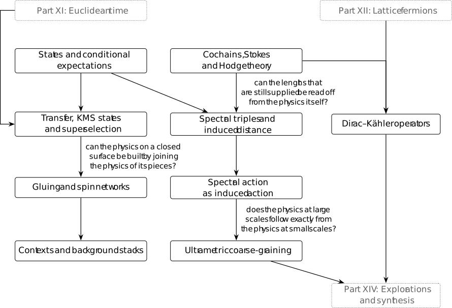
The arrows from Euclidean time enter the transfer chapter; those from lattice fermions enter the Dirac-Kähler chapter. They mark selected intended prerequisites for the chapters below, while the two opening questions motivate the part as a whole. Other suppliers are specified when each construction is developed.
39.1. States and conditional expectations [fdip-008S]AGENTDRAFTED
- November 2, 2026
39.1. States and conditional expectations [fdip-008S]AGENTDRAFTED
- November 2, 2026
Can the physics be rebuilt from its observables alone? This chapter asks how a state on a finite-dimensional algebra determines a Hilbert space.
The first section builds that space from the Gram form \(\omega (a^*b)\). Its dimension is the rank of the Gram matrix. On a direct sum of matrix algebras that rank is the sum of each block size times the rank of the density, and on functions the space is \(\ell ^2\) of the support. No norm on the algebra is assumed. The following section shows that a Wick conditional expectation sends polynomials to polynomials in the retained variables and that nested retained sets compose. The normalized Grassmann state restricts to the state of the Schur complement.
Theorem 39.1.1. Finite *-algebras, states and GNS [fdip-008T]AGENTDRAFTED
- November 2, 2026
Theorem 39.1.1. Finite *-algebras, states and GNS [fdip-008T]AGENTDRAFTED
- November 2, 2026
A state in the sense of the real and complex algebraic states is a normalized positive functional. That note assumes no norm and no operator representation. On a finite-dimensional *-algebra the functional itself determines both. The squared length of a class is the value of the state on \(\,a^*a\), and the dimension of the resulting space is the rank of one Gram matrix.
Let \(K=\mathbb R\) or \(K=\mathbb C\), and let \(A\) be a finite-dimensional unital associative \(K\)-algebra with an involution of the kind fixed for a real algebraic state or a complex algebraic state. Let \(\omega \) be a real or complex algebraic state on \(A\), according to the scalar field: \(K\)-linear, normalized in the sense of a normalized linear functional, Hermitian positive, and satisfying \(\omega (a^*a)\ge 0\). Define \(\langle x,y\rangle =\omega (x^*y)\). Let \(N\) be the set of \(x\) with \(\langle x,x\rangle =0\). The quotient \(H_\omega =A/N\) carries the descended inner product, the operator \(\pi _\omega (a)\) sends the class of \(b\) to the class of \(ab\), and \(\Omega \) is the class of \(1\).
The form is positive semidefinite and Hermitian, and \(N\) is a left ideal. For the cyclic vector, \[\langle \pi _\omega (a)\Omega ,\pi _\omega (b)\Omega \rangle =\omega (a^*b).\] For any basis the Gram matrix \(G_{ij}=\omega (e_i^*e_j)\) has \(\dim H_\omega =\operatorname {rank} G\). The squared length of the class of \(a\) is \(\omega (a^*a)\).
Let \(A=\bigoplus _i M_{m_i}(K)\), with componentwise product and with conjugate transpose acting on each block. Suppose each \(\rho _i\) has the form \(\rho _i=c_i^*c_i\), and \(\sum _i\mathrm {Tr}(\rho _i)=1\). The functional \(\omega (a)=\sum _i\mathrm {Tr}(\rho _i a_i)\) is a state, and \[\dim H_\omega =\sum _i m_i\operatorname {rank}\rho _i.\] On \(M_2\), the density \(\mathrm {diag}(2/3,1/3)\) has rank \(2\) and gives dimension \(4\). The density \(\mathrm {diag}(1,0)\) has rank \(1\) and gives dimension \(2\).
Let \(X\) be a finite set and let \(A\) be the algebra of functions \(X\to K\), with pointwise product and pointwise conjugation. Let \(w:X\to \mathbb R_{\geq 0}\) satisfy \(\sum _x w(x)=1\), and set \(\omega (f)=\sum _x w(x)f(x)\). Write \(\operatorname {supp} w\) for the labels with \(w(x)>0\). Then \(H_\omega \) is the space of all functions on that support, with the inner product weighted by \(w\). On a finite set that space is \(\ell ^2(\operatorname {supp} w)\).
Equivariant precision and real types records, inside a symmetry sector, a matrix over the reals, the complexes or the quaternions. This section does not prove that those matrices are the blocks of a decomposition of the observable algebra.
Proof.
- November 2, 2026
Proof.
- November 2, 2026
The form is linear in the second argument because \(\omega \) is.
It is conjugate-linear in the first because \((\lambda x)^*=\overline \lambda \,x^*\).
It is Hermitian because \(\langle y,x\rangle \) equals \(\omega ((x^*y)^*)\), and Hermitian positivity makes that the conjugate of \(\omega (x^*y)\). The square \(\langle x,x\rangle =\omega (x^*x)\) is nonnegative by the state.
The inequality of Cauchy and Schwarz is \(\lvert \langle x,y\rangle \rvert ^2\le \langle x,x\rangle \langle y,y\rangle \). Over \(\mathbb C\), if \(\langle x,y\rangle \) is not zero, choose a scalar \(u\) of modulus \(1\) with \(u\langle x,y\rangle =\lvert \langle x,y\rangle \rvert \), and replace \(y\) by \(uy\). The new square \(\langle y,y\rangle \) is unchanged, and the new inner product is real and nonnegative. Over \(\mathbb R\) no phase is required. For every real \(t\), \[\langle x+ty,x+ty\rangle =\langle x,x\rangle +2t\langle x,y\rangle +t^2\langle y,y\rangle \ge 0.\] If \(\langle y,y\rangle =0\), the values \(2t\langle x,y\rangle \) cannot stay above \(- \langle x,x\rangle \) for every real \(t\) unless \(\langle x,y\rangle =0\). If \(\langle y,y\rangle >0\), complete the square. The same quadratic is \[\langle y,y\rangle \Bigl (t+\frac {\langle x,y\rangle }{\langle y,y\rangle }\Bigr )^2 +\langle x,x\rangle -\frac {\langle x,y\rangle ^2}{\langle y,y\rangle }.\] The squared term can be made zero, so the remaining term is nonnegative. Thus the inequality holds. Over \(\mathbb C\), putting the unimodular factor back into \(y\) multiplies \(\langle x,y\rangle \) by a scalar of modulus \(1\) and does not change \(\langle y,y\rangle \).
If \(\langle x,x\rangle =0\), the inequality forces \(\langle x,y\rangle =0\) for every \(y\). Conversely the case \(y=x\) shows that the radical is exactly \(N\). It is a subspace. If \(x,y\in N\) and \(\lambda \in K\), then \[\begin {aligned} \langle x+\lambda y,x+\lambda y\rangle ={}&\langle x,x\rangle +\lambda \langle x,y\rangle \\ &+\overline {\lambda }\langle y,x\rangle +\lvert \lambda \rvert ^2\langle y,y\rangle . \end {aligned}\] The two squares vanish because \(x,y\in N\). The two cross terms vanish because an element of \(N\) is orthogonal to every vector. It is a left ideal. For \(b\in A\) and \(x\in N\), \(\langle bx,bx\rangle =\omega (x^*b^*bx)=\langle x,(b^*b)x\rangle =0\).
The form therefore descends to the quotient. If \(x-x'\) and \(y-y'\) lie in \(N\), then \(\langle x,y\rangle -\langle x',y'\rangle =\langle x-x',y\rangle +\langle x',y-y'\rangle \). The first summand vanishes because \(x-x'\) is in the radical. The second is the conjugate of \(\langle y-y',x'\rangle \), which vanishes for the same reason. The descended form is positive definite, and finite dimensionality makes the quotient a Hilbert space with no further completion. Its dimension is \(\dim A-\dim N\).
On a basis \(e_1,\ldots ,e_n\), the matrix \(G_{ij}=\langle e_i,e_j\rangle =\omega (e_i^*e_j)\) is Hermitian. A vector \(v\) represents \(x=\sum _i v_i e_i\). Hermitian symmetry gives \(G_{ji}=\overline {G_{ij}}\). The number \(\langle x,e_j\rangle =\sum _i\overline {v_i}G_{ij}\) vanishes for every \(j\) if and only if \(x\in N\): the forward direction was proved for every vector, and the converse is linearity in the second argument. Conjugating those sums and replacing \(\overline {G_{ij}}\) by \(G_{ji}\) produces \((Gv)_j=0\). Rank-nullity gives \(\operatorname {rank} G=n-\dim N=\dim H_\omega \). The class of \(a\) has squared length \(\omega (a^*a)\). The operator \(\pi _\omega (a)\) is well defined because \(N\) is a left ideal, and \(\langle \pi _\omega (a)\Omega ,\pi _\omega (b)\Omega \rangle =\langle a,b\rangle =\omega (a^*b)\).
On the direct sum, the product and the involution act blockwise, so \(\omega (a^*a)=\sum _i\mathrm {Tr}(\rho _i a_i^*a_i)\). The trace is invariant under a cyclic permutation, and \(\mathrm {Tr}(b^*b)\) is the sum of the squared moduli of the entries of \(b\). Hence \[\mathrm {Tr}(\rho _i a_i^*a_i) =\mathrm {Tr}(c_i a_i^*a_i c_i^*) =\mathrm {Tr}\bigl ((a_i c_i^*)^*(a_i c_i^*)\bigr ),\] which is nonnegative. The functional is therefore positive. It is normalized because \(\omega (1)=\sum _i\mathrm {Tr}(\rho _i)=1\). Each \(\rho _i=c_i^*c_i\) is self-adjoint. The trace of a conjugate transpose is the conjugate of the trace, and \((a_i\rho _i)^*=\rho _i a_i^*\), so \(\mathrm {Tr}(\rho _i a_i^*)=\overline {\mathrm {Tr}(\rho _i a_i)}\). Thus \(\omega \) is Hermitian.
The same identity shows that \(\omega (a^*a)=0\) if and only if \(a_i c_i^*=0\) for every \(i\). Different blocks occupy complementary summands, so \(\dim N=\sum _i\dim \{a_i:a_i c_i^*=0\}\). A matrix vanishes on a subspace precisely when it factors through the quotient by that subspace. The image of \(c_i^*\) has dimension \(\operatorname {rank} c_i^*\). The matrices vanishing on it are determined by their values on a complement, so their space has dimension \(m_i\bigl (m_i-\operatorname {rank} c_i^*\bigr )\). The quotient of that block therefore has dimension \(m_i\operatorname {rank} c_i^*\). Summing over the blocks gives \(\dim H_\omega =\sum _i m_i\operatorname {rank} c_i^*\).
It remains to match that rank with \(\operatorname {rank}\rho _i\). For the standard inner product, \(\|c_i v\|^2=\langle c_i^*c_i v,v\rangle \). If \(c_i^*c_i v=0\), the right-hand side vanishes, so \(c_i v=0\). The converse is immediate, and rank-nullity gives \(\operatorname {rank}\rho _i=\operatorname {rank} c_i\). A minor of a transpose is the transpose of a minor, and the determinant is unchanged by transposition. A minor of a conjugate transpose is the conjugate of a minor of the transpose. The largest size of a nonzero minor is therefore the same for \(c_i\), \(c_i^T\) and \(c_i^*\). Hence \(\operatorname {rank} c_i^*=\operatorname {rank}\rho _i\), and \(\dim H_\omega =\sum _i m_i\operatorname {rank}\rho _i\). On \(M_2\), \(\mathrm {diag}(2/3,1/3)\) is the square of \(\mathrm {diag}(\sqrt {2/3},\sqrt {1/3})\), so its rank is \(2\). \(\mathrm {diag}(1,0)\) is the square of \(\mathrm {diag}(1,0)\), and its only nonzero minor has size \(1\). The formula gives dimensions \(4\) and \(2\).
On functions, the indicator basis is orthogonal for the Gram form. Indeed \(\omega (1_x^*1_y)=\delta _{xy}w(x)\), so the Gram matrix is diagonal with entries \(w(x)\). Its rank is the number of strictly positive weights. A function lies in \(N\) exactly when it vanishes on \(\operatorname {supp} w\), because \(\omega (f^*f)=\sum _x w(x)\lvert f(x)\rvert ^2\). Two functions determine the same class exactly when they agree on that support, and every function on the support arises in this way. The descended inner product is \[\langle f,g\rangle =\sum _{w(x)>0}w(x)\overline {f(x)}\,g(x).\] Every function on a finite set is square-summable, so the space is \(\ell ^2(\operatorname {supp} w)\).
Theorem 39.1.2. Nested conditional expectations compose [fdip-008U]AGENTDRAFTED
- November 2, 2026
Theorem 39.1.2. Nested conditional expectations compose [fdip-008U]AGENTDRAFTED
- November 2, 2026
Let \(A\) be a unital associative algebra and \(\omega \) a linear functional on \(A\). Let \(B\subset A\) be a unital subalgebra. A conditional expectation of \(\omega \) onto \(B\) is a linear map \(E:A\to B\) with \(E(1)=1\), \(E(b_1ab_2)=b_1E(a)b_2\) for \(b_1,b_2\in B\), and \(\omega (E(a))=\omega (a)\). When \(A\) carries the involution of an algebraic state, \(\omega \) is such a state, and \(E(a^*)=E(a)^*\), the same identities give \(\omega (c^*E(a^*a)c)=\omega ((ac)^*(ac))\) for \(c\in B\). No norm on \(A\) enters that identity.
Keep the Wick data of the ring-level moment theorem: \(2\) is a unit, \(Q\) is symmetric and invertible, and \(E_T\) denotes the substitution map of that note onto a retained set \(T\), defined whenever the eliminated block is invertible. For retained sets \(R\subset R'\), write \(U'\) for the complement of \(R'\) and \(V\) for the coordinates in \(R'\) but not in \(R\). Let \(S'\) be the Schur complement of \(Q\) after eliminating \(U'\), and assume that \(Q_{U'U'}\) and the block \((S')_{VV}\) are invertible.
Then \(E_R\) is a conditional expectation of \(\omega _Q\) onto \(A[x_R]\). The two maps compose, \[E_R\circ E_{R'}=E_R.\] On the four-cycle of the moment note, the conditional expectation of the displayed quartic lies in \(\mathbb Q[x_0,x_1]\), and the common value of the two Wick functionals is \(32/75\).
Let \(K\) be an invertible complex matrix, ordered as in the Grassmann Schur formula, with invertible eliminated block \(D\) and Schur complement \(S\). Let \(F\) be a polynomial in the retained paired generators. The normalized state \[\omega _K(F)=\frac {J_n(F e^{-\bar \psi K\psi })}{\det K}\] restricts by \[\omega _K(F)=\omega _S(F).\] Thus the retained state is the normalized Grassmann state of \(S\).
Proof.
- November 2, 2026
Proof.
- November 2, 2026
The constant \(1\) does not involve the residual indeterminates, and the Wick value of \(1\) is \(1\), so \(E_R(1)=1\). A polynomial \(g\in A[x_R]\) is a coefficient for the residual Wick functional. That functional is linear over \(A[x_R]\), hence \(E_R(gf)=gE_R(f)\). The polynomial ring is commutative, so the two sides of the bimodule identity agree. The moment theorem gives \(\omega _Q(h)=\omega _Q(E_R(h))\) for every polynomial \(h\). Taking \(h=gf\) yields \(\omega _Q(gE_R(f))=\omega _Q(gf)\). The image lies in \(A[x_R]\) by that same theorem.
Apply the moment theorem to the partition \((R',U')\). The residual \(z'=x_{U'}+L'x_{R'}\) is uncorrelated with \(x_{R'}\), and its covariance is \(Q_{U'U'}^{-1}\). The same theorem, applied to the invertible precision \(S'\) and the partition \((R,V)\), produces a residual \(z_V\) in the variables \(x_{R'}\) whose covariance is \((S')_{VV}^{-1}\) and which is uncorrelated with \(x_R\). Second moments of polynomials in \(x_{R'}\) agree under \(\omega _Q\) and under the Wick state of \(S'\), so these two covariances are the moments of \(\omega _Q\). Since \(z_V\) is linear in \(x_{R'}\) and \(z'\) is uncorrelated with \(x_{R'}\), one has \(\omega _Q(z_Vz')=0\).
The moment theorem defines the Schur complement after eliminating \(U'\) by \(S'=Q_{R'R'}-Q_{R'U'}Q_{U'U'}^{-1}Q_{U'R'}\). Its block on \(V\) is therefore \((S')_{VV}=Q_{VV}-Q_{VU'}Q_{U'U'}^{-1}Q_{U'V}\). The same expression is the Schur complement of the invertible block \(Q_{U'U'}\) inside \(Q_{UU}\). That theorem says that, once the eliminated block is invertible, the block matrix is invertible if and only if that Schur complement is. Both are invertible, so \(Q_{UU}\) is invertible, and the one-step map \(E_R\) is defined. Substitute \[x_V=B_Vx_R+z_V\] and then \[x_{U'}=B'x_{R'}+z'.\] The second substitution expands to a retained linear form plus \(B'_Vz_V+z'\). In residual coordinates the change of variables is \[z_U= \begin {pmatrix}I&0\\ B'_V&I\end {pmatrix} \begin {pmatrix}z_V\\ z'\end {pmatrix}.\] The triangular factor has determinant \(1\) and an inverse over \(A\). Both \(z_V\) and \(z'\) are uncorrelated with \(x_R\), so the residual is uncorrelated with \(x_R\). Its retained coefficient is therefore the regression of the moment theorem: the covariance \(C_{RR}\) is invertible, and \(C(x_U,x_R)=BC_{RR}\) determines that coefficient. The one-step residual \(z_U\) is this triangular image.
A pairing in the joint residual that joins \(z_V\) to \(z'\) contributes \(0\). Every surviving pairing is a \(z_V\) pairing times a \(z'\) pairing, so the joint Wick average is the iterated average. The polynomial obtained after the two substitutions is the same polynomial of \(z_U\), and Isserlis' rule depends only on the pairwise covariances of those linear forms. Substitution of \(x_V=B_Vx_R+z_V\) is a ring homomorphism, and the residual Wick functional is linear on coefficients, so the \(z'\) average commutes with that substitution. The average in \(z'\) alone is \(E_{R'}(f)\). Once that polynomial no longer involves \(z'\), the one-step residual average uses only \(z_V\), with covariance \((S')_{VV}^{-1}\). On \(A[x_{R'}]\) that average is \(E_R\). The iterated average is therefore \(E_R(E_{R'}(f))\), and it equals \(E_R(f)\).
For the Grassmann state, the exponential is a sum of even elements. An even element commutes with every homogeneous element, by the Grassmann algebra. The eliminated top word is even, so passing it through the retained polynomial \(F\) contributes no sign. The partial coefficient formula therefore gives \[J_U(F e^{-\bar \psi K\psi }) =\det (D)\,F e^{-\bar \psi _R S\psi _R}.\] Applying \(J_R\) and dividing by \(\det K=\det (D)\det S\) produces \(\omega _S(F)\). The scalar conventions of the empty blocks remain those of the partial formula.
The block factorization used above is the same matrix identity
recorded for the moment theorem. TauCeti's
Matrix.PosDef.gaussianCondCov remains the real
positive-definite covariance, not this tower over a ring. No Mathlib
declaration was found for the Isserlis composition or for the
normalized Grassmann restriction.
No norm-one projection theorem is proved here. Tomiyama's paper of 1957 has not been read. The identities above do not use a norm on the algebra. They also do not identify the Grassmann state with a state on the configuration Clifford algebra.
39.2. Transfer, KMS states and superselection [fdip-008V]AGENTDRAFTED
- November 1, 2026
39.2. Transfer, KMS states and superselection [fdip-008V]AGENTDRAFTED
- November 1, 2026
How do time evolution and symmetry appear in the language of observables and states? The first section shows that the crossing block of a positive definite precision sets the rank of the linear reflection Gram, and that a finite Gibbs state obeys the conjugation identity. The Gaussian and gauge transfer operators remain the positive operators already constructed for those systems.
The following section asks which observables remain when a symmetry is imposed.
Theorem 39.2.1. The crossing block sets the reflection rank [fdip-008W]AGENTDRAFTED
- November 2, 2026
Theorem 39.2.1. The crossing block sets the reflection rank [fdip-008W]AGENTDRAFTED
- November 2, 2026
Let \(Q\) be a real symmetric positive definite matrix, partitioned into blocks \(Q_{++}\), \(Q_{+-}\), \(Q_{-+}\) and \(Q_{{-}{-}}\), and let \(C=Q^{-1}\). Principal submatrices of a positive definite matrix are positive definite, so \(Q_{++}\) and \(C_{{-}{-}}\) are invertible, and \[\operatorname {rank}C_{+-}=\operatorname {rank}Q_{+-}.\]
On the even torus of the reflection halves, with the spatial factor a point, take the link reflection and the massive scalar law of nearest-neighbor weight \(1\) and mass \(m>0\). The linear reflection Gram matrix, indexed by the positive-half coordinates, has rank \(2\) and is positive semidefinite. The normalized Gaussian transfer operator remains the injective positive contraction of the Hermite diagonalization. The gauge transfer operator remains positive, injective and trace class, as proved for the spatial transfer data.
Let \(H\) be an \(n\times n\) Hermitian matrix and let \(\beta \) be real. The exponential series of a finite matrix converges entrywise. Write \(\rho =e^{-\beta H}/Z\) with \(Z=\operatorname {Tr}(e^{-\beta H})\), and write \(\sigma (A)=e^{-\beta H}Ae^{\beta H}\). The Gibbs state \(\omega (A)=\operatorname {Tr}(\rho A)\) satisfies \[\omega (AB)=\omega (B\sigma (A)).\]
Proof.
- November 2, 2026
Proof.
- November 2, 2026
If \(v\) is a nonzero vector in the first block of coordinates, extend it by zero on the second block. Positive definiteness of \(Q\) gives \(v^TQ_{++}v>0\), so \(Q_{++}\) is positive definite. If \(v\) is a nonzero vector supported on the minus coordinates, extend it by zero on the plus coordinates. Positive definiteness of \(C\) gives \(v^TC_{{-}{-}}v>0\), so \(C_{{-}{-}}\) is positive definite. The off-diagonal block of \(QC=I\) is \[Q_{++}C_{+-}+Q_{+-}C_{{-}{-}}=0.\] Hence \[C_{+-}=-Q_{++}^{-1}Q_{+-}C_{{-}{-}}.\] Left multiplication by the invertible matrix \(Q_{++}^{-1}\) and right multiplication by the invertible matrix \(C_{{-}{-}}\) preserve rank, so the two blocks have the same rank.
For the cycle, the positive half is \(\{1,\ldots ,M\}\) and its image under \(\theta _\ell (t)=1-t\) is the complementary half, with \(M\ge 2\) and length \(2M\). The quadratic form of the massive scalar law has off-diagonal entry \(-1\) on each nearest-neighbor edge and no other off-diagonal entry. The only edges with one end in each half are \(\{0,1\}\) and \(\{M,M+1\}\). Their rows in the positive half are the distinct sites \(1\) and \(M\), and their columns in the negative half are the distinct sites \(0\) and \(M+1\). The crossing block therefore has rank \(2\). The covariance crossing block has the same rank. For real coordinate functions \(x_a\) on the positive half, \(\Theta x_a=x_{\theta (a)}\), so the reflection Gram matrix is that crossing block of \(C\) with columns ordered by \(\theta \). Its rank is \(2\). Every positive-half polynomial lies in the reflection-positive domain of the massive scalar law, so the Gram matrix is positive semidefinite.
Let \(\mu \) bound the absolute values of the entries of \(H\). By induction, the entries of \(H^k\) are at most \(n^{k-1}\mu ^k\). The exponential series is therefore dominated by a scalar exponential and converges entrywise. Since \(H\) commutes with \(-H\), the Cauchy product of the series for \(e^{\beta H}\) and \(e^{-\beta H}\) is the series for \(e^{0}\), which is the identity. The coefficients are real and \(H^*=H\), so \(e^{-\beta H}\) is Hermitian. The same product of series gives \(e^{-\beta H}=e^{-\beta H/2}e^{-\beta H/2}\). For a column \(v\), the squared length \(v^*e^{-\beta H}v\) vanishes only if \(e^{-\beta H/2}v=0\), hence only if \(v=0\). The exponential is positive definite, so its trace \(Z\) is positive. For finite matrices \(\operatorname {Tr}(XY)=\operatorname {Tr}(YX)\). Cycling the first factor gives \[\operatorname {Tr}(e^{-\beta H}Be^{-\beta H}Ae^{\beta H}) =\operatorname {Tr}(Be^{-\beta H}A),\] and cycling \(B\) gives \(\operatorname {Tr}(e^{-\beta H}AB)\). Dividing by \(Z\) is the identity for \(\omega \).
The rank identity uses no reflection. Reflection positivity of the cycle is the massive scalar theorem already cited, and the transfer operators are the two theorems already cited. No infinite volume, no continuum limit, and no claim that the finite Gibbs identity determines a modular operator beyond the displayed conjugation are made here.
Theorem 39.2.2. The fixed-point algebra is the averaged image [fdip-008X]AGENTDRAFTED
- November 2, 2026
Theorem 39.2.2. The fixed-point algebra is the averaged image [fdip-008X]AGENTDRAFTED
- November 2, 2026
Let \(K\) be \(\mathbb R\) or \(\mathbb C\), and let \(A\) be a unital associative \(K\)-algebra. A symmetry of a linear functional \(\omega \) on \(A\) is a unital \(K\)-algebra automorphism \(\alpha \) with \(\omega (\alpha (a))=\omega (a)\) for every \(a\). Let \(G\) be a finite group, and let \(g\mapsto \alpha _g\) be a homomorphism from \(G\) into the unital \(K\)-algebra automorphisms of \(A\), so that \(\alpha _{hg}=\alpha _h\circ \alpha _g\). The order \(|G|\) is invertible in \(K\). Define \[E(a)=\frac 1{|G|}\sum _{g\in G}\alpha _g(a).\] Write \(A^G\) for the fixed-point algebra, the elements fixed by every \(\alpha _g\). Then \(E\) is linear, \(E(1)=1\), the image of \(E\) is \(A^G\), and \(E(b_1ab_2)=b_1E(a)b_2\) whenever \(b_1\) and \(b_2\) are fixed. If every \(\alpha _g\) preserves \(\omega \), then \(\omega (E(a))=\omega (a)\). These are the identities of a conditional expectation of \(\omega \) onto \(A^G\). If every \(\alpha _g\) preserves an involution of \(A\), then \(E(a^*)=E(a)^*\).
When the automorphisms are conjugations \(\alpha _g(R)=\rho (g)R\rho (g)^{-1}\) by a representation \(\rho \) on a finite-dimensional space, the fixed-point algebra is the commutant of \(\rho (G)\). On the half-turn of Proposition 11.9, with \(P=\operatorname {diag}(I_2,-I_2)\) and \(R\) written in those blocks as \(\begin {pmatrix}A&B\\C&D\end {pmatrix}\), the average is the block-diagonal operator \[E(R)=\begin {pmatrix}A&0\\0&D\end {pmatrix}.\] That note identifies this commutant with \(M_2(\mathbb R)\times M_2(\mathbb R)\) and records that the image of the group algebra is the smaller algebra of scalar blocks.
The neutral Gauss constraint for a finite gauge group asks for the link functions fixed by every group element, and its projector is this same average. An invariant functional therefore satisfies \(\omega =\omega \circ E\): its value depends on an observable only through the averaged observable. The charged space remains the intertwiner space of Theorem 34.3. The multiplicity matrices of a real orthogonal action remain the commutant description of Theorem 13.1.
Proof.
- November 2, 2026
Proof.
- November 2, 2026
Each \(\alpha _g\) is \(K\)-linear, so \(E\) is linear. A unital automorphism fixes \(1\), and therefore \(E(1)=1\).
For \(h\in G\), \[\alpha _h(E(a)) =\frac 1{|G|}\sum _{g\in G}\alpha _h(\alpha _g(a)) =\frac 1{|G|}\sum _{g\in G}\alpha _{hg}(a).\] As \(g\) runs through \(G\), so does \(hg\). Hence \(\alpha _h(E(a))=E(a)\), and the image of \(E\) lies in \(A^G\).
If \(b\) is fixed by every \(\alpha _g\), every summand equals \(b\), so \(E(b)=b\). Thus \(A^G\) is contained in the image, and \(E\) is the identity on \(A^G\). The two inclusions give \[A^G=\operatorname {im}E.\]
Let \(b_1\) and \(b_2\) be fixed. Multiplicativity gives \(\alpha _g(b_1ab_2)=\alpha _g(b_1)\alpha _g(a)\alpha _g(b_2) =b_1\alpha _g(a)b_2\). Averaging both sides yields \(E(b_1ab_2)=b_1E(a)b_2\).
If every \(\alpha _g\) preserves \(\omega \), then \(\omega (\alpha _g(a))=\omega (a)\). Averaging the scalar values gives \(\omega (E(a))=\omega (a)\). If every automorphism preserves an involution, \(\alpha _g(a^*)=\alpha _g(a)^*\), and the same average gives \(E(a^*)=E(a)^*\).
For a conjugation action, \(\alpha _h(E(R))=E(R)\) is the statement that \(E(R)\) commutes with every \(\rho (h)\). If \(R\) already lies in the commutant, the preceding paragraph gives \(E(R)=R\). Thus the image is exactly the commutant.
In the half-turn coordinates the conjugation by \(P=\operatorname {diag}(I_2,-I_2)\) sends \(\begin {pmatrix}A&B\\C&D\end {pmatrix}\) to \(\begin {pmatrix}A&-B\\-C&D\end {pmatrix}\). The average of the two operators is the displayed block-diagonal matrix. The identification of that commutant, and the comparison with the group-algebra image, are the calculations of Proposition 11.9.
Tomiyama's norm-one projection theorem has not been read, and no norm on \(A\) is used. The argument gives the finite average only. It does not identify the sectors with the centre of the commutant, and it does not replace the charged intertwiner description.
39.3. Cochains, Stokes and Hodge theory [fdip-008Y]AGENTDRAFTED
- November 2, 2026
39.3. Cochains, Stokes and Hodge theory [fdip-008Y]AGENTDRAFTED
- November 2, 2026
What replaces a derivative when the only space is a grid? The zero-mode count for the centered Dirac operator gives \(\dim _{\mathbb C}\ker D=2^{d+e}\), where \(e\) is the number of even periods among \(N_1,\ldots ,N_d\). For \(d=2\) that dimension is \(2^{2+e}\), so it changes when a side length changes parity.
The square cell complex on the same vertices does not. For every pair of positive integers, the coboundary composed with itself is zero and the real cohomology has dimensions \((1,2,1)\). The following section takes up the adjoint of this coboundary.
Theorem 39.3.1. Square tori have Betti numbers (1, 2, 1) [fdip-008Z]AGENTDRAFTED
- November 2, 2026
Theorem 39.3.1. Square tori have Betti numbers (1, 2, 1) [fdip-008Z]AGENTDRAFTED
- November 2, 2026
Let \(N_1\) and \(N_2\) be positive integers, and set \(V=N_1N_2\). The vertices are the \(V\) pairs \((x,y)\) of integers modulo \(N_1\) and \(N_2\), with addition of coordinates taken modulo those side lengths. For each vertex there is a horizontal edge \(e^h_{x,y}\) from \((x,y)\) to \((x+1,y)\), a vertical edge \(e^v_{x,y}\) from \((x,y)\) to \((x,y+1)\), and a face \(\sigma _{x,y}\). When a side length equals \(1\), each edge in that direction is a loop. The boundary of the face is \[\partial \sigma _{x,y} =e^h_{x,y}+e^v_{x+1,y}-e^h_{x,y+1}-e^v_{x,y}.\]
Real cochains are real functions on these cells. Write \(C^0\), \(C^1\) and \(C^2\) for the functions on vertices, edges and faces, of dimensions \(V\), \(2V\) and \(V\). A chain is a real linear combination of cells of one dimension, and the evaluation pairing \(\langle \beta ,c\rangle \) sums the pointwise products of a cochain with the coefficients of a chain. The coboundary \(d\) is the transpose of the boundary, in the sense that \(\langle d\beta ,c\rangle =\langle \beta ,\partial c\rangle \) whenever the degrees match. On vertex functions this is the incidence map of the ring-valued incidence: \((df)(e)=f(h(e))-f(s(e))\). In coordinates, \[\begin {aligned} (d_0f)^h(x,y)&=f(x+1,y)-f(x,y),\\ (d_0f)^v(x,y)&=f(x,y+1)-f(x,y),\\ (d_1\alpha )(\sigma _{x,y}) &=\alpha ^h(x,y)+\alpha ^v(x+1,y) -\alpha ^h(x,y+1)-\alpha ^v(x,y). \end {aligned}\]
The composite \(d_1\circ d_0\) is zero. Write \(b_0\) for the dimension of \(\ker d_0\), write \(b_1\) for the dimension of the quotient of \(\ker d_1\) by the image of \(d_0\), and write \(b_2\) for the dimension of the quotient of \(C^2\) by the image of \(d_1\). These Betti numbers are \(1\), \(2\) and \(1\).
Proof.
- November 2, 2026
Proof.
- November 2, 2026
Substitute the coordinate formulas. At the face \(\sigma _{x,y}\), \[\begin {aligned} (d_1d_0f)(\sigma _{x,y}) &=\bigl (f(x+1,y)-f(x,y)\bigr )\\ &\quad +\bigl (f(x+1,y+1)-f(x+1,y)\bigr )\\ &\quad -\bigl (f(x+1,y+1)-f(x,y+1)\bigr )\\ &\quad -\bigl (f(x,y+1)-f(x,y)\bigr ). \end {aligned}\] The 8 terms cancel in pairs, so \(d_1d_0f=0\). The pairing separates chains, and therefore the boundary of every face boundary is zero as well.
If \(d_0f=0\), then \(f(x+1,y)=f(x,y)\) and \(f(x,y+1)=f(x,y)\) for every vertex. Following the horizontal steps from \((0,0)\) and then the vertical steps gives \(f(x,y)=f(0,0)\). The kernel consists of the constant functions, so \(\dim \ker d_0=1\) and the rank of \(d_0\) is \(V-1\).
On a single cycle of length \(N\ge 1\), a real function \(g\) on the residues modulo \(N\) is the coboundary of a vertex function if and only if the sum of its values is zero. The forward difference of any vertex function sums to zero. Conversely, if that sum vanishes, set \(f(0)=0\) and let \(f(k)\) be the sum of \(g(0),\ldots ,g(k-1)\) for \(1\le k\le N-1\), with the empty sum equal to zero when \(N=1\). For \(0\le k\le N-2\) the forward difference equals \(g(k)\). The remaining difference is \(f(0)-f(N-1)\). It equals the negative of the sum of \(g(0),\ldots ,g(N-2)\), which the vanishing-sum hypothesis rewrites as \(g(N-1)\). When \(N=1\) both that difference and \(g(0)\) are zero. Thus \(g\) is a coboundary. The functions with vanishing difference are the constants, a one-dimensional space, so the coboundary on the cycle has rank \(N-1\).
Let \(\alpha \) satisfy \(d_1\alpha =0\). Write \(P^h(y)=\sum _x\alpha ^h(x,y)\) and \(P^v(x)=\sum _y\alpha ^v(x,y)\). Sum the face equation over \(x\). The vertical terms cancel because \(x+1\) runs through every residue, and the result is \(P^h(y)=P^h(y+1)\). Sum the face equation over \(y\). The horizontal terms cancel, and the result is \(P^v(x)=P^v(x+1)\). Thus both quantities are constants; call them \(P^h\) and \(P^v\). If \(\alpha =d_0f\), each is a sum of a telescoping difference, so \((P^h,P^v)=(0,0)\).
Conversely, suppose \(d_1\alpha =0\) and \((P^h,P^v)=(0,0)\). For each fixed \(y\), the horizontal row sums to zero, so the cycle criterion supplies a function \(f(\cdot ,y)\) with \(f(0,y)=0\) and horizontal difference \(\alpha ^h\). Define \(\delta (x,y)=\alpha ^v(x,y)-\bigl (f(x,y+1)-f(x,y)\bigr )\). Its horizontal difference is \[\alpha ^v(x+1,y)-\alpha ^v(x,y) -\bigl (\alpha ^h(x,y+1)-\alpha ^h(x,y)\bigr ).\] The face equation rearranges to the vanishing of that expression. Hence \(\delta (x,y)\) depends only on \(y\). The normalization \(f(0,y)=0\) gives the common value \(k(y)=\alpha ^v(0,y)\). The sum of \(k\) is \(P^v=0\), so the cycle criterion supplies \(c\) with \(c(y+1)-c(y)=k(y)\). The function \(f(x,y)+c(y)\) then has horizontal difference \(\alpha ^h\) and vertical difference \(\alpha ^v\). Every cocycle with vanishing periods is therefore a coboundary.
The identity \(d_1d_0=0\) puts the image of \(d_0\) inside \(\ker d_1\). Coboundaries have vanishing periods, and every cocycle with vanishing periods is a coboundary, so that image is exactly the set of cocycles whose periods vanish. The edge field with every horizontal value \(1\) and every vertical value \(0\) has coboundary zero on each face, because the face sees \(+1\) on its lower edge and \(-1\) on its upper edge. Its periods are \((N_1,0)\). The field with the two roles exchanged is likewise a cocycle, with periods \((0,N_2)\). For real \(a\) and \(b\), the combination with horizontal value \(a/N_1\) and vertical value \(b/N_2\) is a cocycle of periods \((a,b)\). The period map on \(\ker d_1\) is therefore a surjective linear map to \(\mathbb R^2\), with kernel equal to the image of \(d_0\). Rank nullity gives \[\dim \ker d_1=(V-1)+2=V+1,\] and the quotient dimension is \[b_1=(V+1)-(V-1)=2.\] The rank of \(d_1\) is \(2V-(V+1)=V-1\).
Summing a coboundary over every face cancels: each horizontal value appears once with each sign as \(y\) runs through a full set of residues, and each vertical value does the same as \(x\) does. The sum of the face values is therefore a linear functional vanishing on the image of \(d_1\). The constant function \(1\) has sum \(V\ne 0\), so the functional is nonzero, its kernel has dimension \(V-1\), and that constant is not a coboundary. The image already has dimension \(V-1\), so the image equals the kernel of the sum. Therefore \(b_2=1\).
The constant vertex functions span the degree-zero cohomology. The two edge fields just named have linearly independent periods, and the degree-one quotient is two-dimensional, so their classes form a basis: one winds around the first coordinate and the other winds around the second. The constant face functions span the degree-two cohomology.
Theorem 39.3.2. Harmonic cochains realize the Betti numbers [fdip-0090]AGENTDRAFTED
- November 2, 2026
Theorem 39.3.2. Harmonic cochains realize the Betti numbers [fdip-0090]AGENTDRAFTED
- November 2, 2026
Let the square torus, its coboundary \(d\), and its evaluation pairing be those of the Betti count. There is no cell below a vertex or above a face, so the coboundary of a face function is zero and there is no adjoint into a vertex from a lower cell. Write \(d^\dagger \) for the adjoint of each coboundary in the evaluation pairing: \(\langle d\gamma ,\beta \rangle =\langle \gamma ,d^\dagger \beta \rangle \). On edge fields this is the counting adjoint. The pairing is symmetric, so \(d\) and \(d^\dagger \) are adjoints of one another, and \(d+d^\dagger \) is self-adjoint. The adjoint of the zero map is zero, and the adjoint reverses composition, so \(d\circ d=0\) gives \(d^\dagger \circ d^\dagger =0\).
On a cochain \(\gamma \) of one degree, define \(\Delta \gamma =d(d^\dagger \gamma )+d^\dagger (d\gamma )\), with either summand omitted when its map has no cells to land on. Call \(\Delta \) the Hodge Laplacian, and call \(\gamma \) harmonic when \(\Delta \gamma =0\). Then \(\Delta =(d+d^\dagger )\circ (d+d^\dagger )\) on each degree. On vertex functions, and with every edge weight equal to \(1\), \(\Delta \) is the unit-weight case of the weighted graph Laplacian. The harmonic cochains in each degree realize the cohomology of that degree, so their dimensions are the Betti numbers \((1,2,1)\). The kernel of \(d+d^\dagger \) therefore has dimension \(4\). A vertex function is the adjoint of an edge field if and only if the sum of its values is zero.
Proof.
- November 2, 2026
Proof.
- November 2, 2026
On a cochain of one degree the two summands of \((d+d^\dagger )\circ (d+d^\dagger )\) are \(d(d^\dagger \gamma )\) and \(d^\dagger (d\gamma )\), because \(d\circ d\) and \(d^\dagger \circ d^\dagger \) vanish. Thus the square is \(\Delta \). Self-adjointness gives \(\langle \Delta \Phi ,\Phi \rangle =\langle (d+d^\dagger )\Phi ,(d+d^\dagger )\Phi \rangle \) for a sum \(\Phi \) of cochains of all three degrees. Expanding the degree-wise formula gives \[\langle \Delta \gamma ,\gamma \rangle =\langle d\gamma ,d\gamma \rangle +\langle d^\dagger \gamma ,d^\dagger \gamma \rangle .\] Both summands are nonnegative, so \(\Delta \gamma =0\) if and only if \(d\gamma =0\) and \(d^\dagger \gamma =0\). The same identity shows that \((d+d^\dagger )\Phi =0\) if and only if every degree of \(\Phi \) is harmonic.
On vertex functions the incoming adjoint is zero, so \(\Delta f=d^\dagger (df)\). The counting adjoint on edge fields is this \(d^\dagger \), and for the constant weight \(1\) the weighted graph Laplacian is \(d_R^\dagger d_R\). The two operators agree.
Fix a degree, and write \(d_-\) for the coboundary into that degree. Its image is contained in the kernel of the outgoing coboundary, because \(d\circ d=0\). The rank of \(d_-^\dagger \) equals the rank of \(d_-\), so the kernel of the adjoint has dimension equal to the dimension of the cochain space minus that rank. Added to the dimension of the image, the total is the whole space. If \(d_-\alpha \) lies in the kernel of \(d_-^\dagger \), then \(\langle d_-\alpha ,d_-\alpha \rangle =\langle \alpha ,d_-^\dagger d_-\alpha \rangle =0\), so \(d_-\alpha =0\). The image therefore meets that kernel only at zero, and the cochain space is their direct sum. A closed cochain splits uniquely as \(d_-\alpha +\rho \) with \(d_-^\dagger \rho =0\). The outgoing coboundary kills \(d_-\alpha \) and kills the sum, so it kills \(\rho \). Thus \(\rho \) is harmonic. The splitting of the closed cochains is direct, and the dimension of the harmonic space is the Betti number of that degree.
On vertices the kernel of \(d\) is the constants. The Betti count gives that kernel dimension \(1\), so the rank of \(d\) is one less than the number of vertices. The image of \(d^\dagger \) from edge fields is orthogonal to that kernel, because \(\langle d^\dagger \alpha ,f\rangle =\langle \alpha ,df\rangle \). The rank of this adjoint equals the rank of \(d\), so the image is the orthogonal complement of the constants. The pairing of a vertex function against the constant \(1\) is the sum of its values, and therefore the complement is the set of vertex functions whose values sum to zero.
The constant vertex functions are harmonic. The two winding edge fields of the Betti count are closed, and each vertex is the head of one edge and the source of one edge in the direction of the winding, with equal values, so the counting-adjoint formula gives zero. The sum of the face values of every coboundary is zero, so the constant face function is orthogonal to every coboundary and its adjoint vanishes. The 4 cochains lie in the three degrees, and the two edge fields are not scalar multiples of one another, so they are linearly independent. The kernel has dimension \(4\), and therefore they form a basis.
39.4. Dirac–Kähler operators [fdip-0091]AGENTDRAFTED
- November 2, 2026
39.4. Dirac–Kähler operators [fdip-0091]AGENTDRAFTED
- November 2, 2026
The centered Dirac operator on a periodic grid has kernel dimension \(2^{d+e}\), where \(e\) counts the even periods. On a square torus that dimension changes when a side length changes parity. The operator built from the coboundary does not. On every square torus the kernel of \(d+d^\dagger \) has dimension \(4\).
The exterior algebra of a free module carries a multiplication and a contraction for each basis vector. No quadratic form enters those two operations. Their ordered products are every linear endomorphism of the algebra, and the sums of matching pairs obey the Clifford relation of the standard dot product. The following section proves both statements. The section after it takes up the product of cochains.
Theorem 39.4.1. Ordered exterior operators span the endomorphisms [fdip-0092]AGENTDRAFTED
- November 2, 2026
Theorem 39.4.1. Ordered exterior operators span the endomorphisms [fdip-0092]AGENTDRAFTED
- November 2, 2026
On every square torus the kernel of \(d+d^\dagger \) has dimension \(4\), by the Hodge theorem. For periods at least \(3\), the centered Dirac operator has kernel dimension \(2^{2+e}\). That dimension equals \(4\) when both periods are odd, and it is strictly larger when either period is even.
Let \(k\) be a commutative ring and let \(n\) be a positive integer. Write \(\bigwedge \) for the exterior algebra of the free module on basis vectors \(e_1,\ldots ,e_n\), with basis the monomials \(e_I\) indexed by subsets \(I\), written in increasing order, and with \(e_\varnothing =1\). Exterior multiplication and contraction along the basis are the linear operators \[\epsilon _i(e_I)=e_i\wedge e_I,\] \[\iota _i(e_I)=0\] when \(i\notin I\), and, when \(i\) occupies position \(p\) in \(I\), \[\iota _i(e_I)=(-1)^p e_{I\setminus \{i\}}.\] For subsets \(S\) and \(T\), write \(\epsilon _S\) and \(\iota _T\) for the compositions of these operators in increasing index order, the largest index acting first, and write \(M_{S,T}=\epsilon _S\circ \iota _T\). There are \(2^n\) choices for each subset, hence \(4^n\) such operators, and they are a basis of the endomorphism ring of \(\bigwedge \). In particular \(\gamma _i=\epsilon _i+\iota _i\) satisfies \[\gamma _i\gamma _j+\gamma _j\gamma _i=2\delta _{ij}I.\] The configuration Clifford algebra is the square quotient of a supplied quadratic form. The operators here are defined before any such form, and the displayed relation is the square relation of the standard dot product. The note does not claim that the resulting Clifford representation is injective.
Proof.
- November 2, 2026
Proof.
- November 2, 2026
The dimension \(4\) is the kernel dimension in the Hodge theorem. The centered count is the cited formula at \(d=2\). It equals \(4\) when \(e=0\). When \(e\ge 1\) the factor \(2^e\) makes it strictly larger. The two statements have the scopes already named.
The monomials are a basis, so operator identities may be checked on \(e_I\). If \(i\in I\), then \(e_i\wedge e_I=0\). If \(i\notin I\) and \(q\) indices of \(I\) are smaller than \(i\), then \(e_i\wedge e_I=(-1)^q e_{I\cup \{i\}}\). Thus \(\epsilon _i^2=0\). For \(i\ne j\) the wedge of the two basis vectors changes sign when their order is exchanged, so \(\epsilon _i\epsilon _j+\epsilon _j\epsilon _i=0\). A monomial contains \(i\) at most once, so \(\iota _i^2=0\).
For the contractions, take \(i\ne j\) and suppose both lie in \(I\), with positions \(p\) and \(r\) and with \(i<j\), so \(p<r\). Removing \(j\) first contributes \((-1)^r\), and \(i\) is still at position \(p\), so the second removal contributes \((-1)^p\). Removing \(i\) first contributes \((-1)^p\), after which \(j\) stands one place earlier, and the second removal contributes \((-1)^{r-1}\). The two signs are opposite, and the remaining monomial is the same. If either index is missing, both double contractions vanish. Hence \(\iota _i\iota _j+\iota _j\iota _i=0\).
Now compare \(\iota _j\epsilon _i\) with \(\epsilon _i\iota _j\). If \(i\ne j\) and \(j\notin I\), the contraction of the input is zero. Exterior multiplication either vanishes or produces a monomial that still omits \(j\), so the later contraction vanishes as well. If \(j\in I\) and \(i\in I\), exterior multiplication of the input vanishes, and the contraction still leaves \(i\) in place, so the later exterior multiplication vanishes. The remaining pattern is \(j\in I\) and \(i\notin I\). Let \(p\) be the position of \(j\) and let \(q\) be the number of indices of \(I\) smaller than \(i\). Removing \(j\) contributes \((-1)^p\). If \(i<j\), wedging \(e_i\) back contributes the same sign \((-1)^q\) that \(e_i\wedge e_I\) carries, while the later removal of \(j\) from \(I\cup \{i\}\) contributes \((-1)^{p+1}\), because \(i\) stands before \(j\). If \(i>j\), wedging \(e_i\) after the removal contributes \((-1)^{q-1}\), because \(j\) was one of the indices counted by \(q\), while the removal of \(j\) from \(I\cup \{i\}\) still contributes \((-1)^p\). In both subcases the two compositions land on the same monomial with opposite signs. If \(i=j\) and \(i\notin I\), the contraction of the input vanishes and \(\iota _i\epsilon _i\) returns \(e_I\), and the product of the two signs \((-1)^q\) is \(1\). If \(i\in I\), exterior multiplication of the input vanishes and \(\epsilon _i\iota _i\) returns \(e_I\), and the product of the two signs \((-1)^p\) is \(1\). Therefore \(\epsilon _i\iota _j+\iota _j\epsilon _i=\delta _{ij}I\).
The square of \(\gamma _i\) is \(\epsilon _i\iota _i+\iota _i\epsilon _i=I\). For \(i\ne j\) each of the 4 pairs in the expansion of \(\gamma _i\gamma _j+\gamma _j\gamma _i\) anticommutes, so the sum is zero. This is the displayed Clifford relation.
The monomials are a free basis, so the endomorphism ring is free on the operators that send one monomial to one monomial and kill the rest. Order the pairs of subsets so that the cardinality of \(T\) increases, and index both the operators \(M_{S,T}\) and these monomial matrix units by that order. The coefficient of \(e_S\) in \(M_{S',T'}e_T\) can be nonzero only when \(T'\subseteq T\). A column with a strictly larger second set therefore does not meet this row. When the cardinalities are equal, necessarily \(T'=T\). The contraction \(\iota _T\) removes every factor of \(e_T\). Each removal meets a present factor, so the image of the contraction is \((\pm 1)\,1\). The following exterior product inserts the factors in \(S'\), each into a monomial that does not yet contain it, and the image is \((\pm 1)\,e_{S'}\). The coefficient of \(e_S\) is therefore zero unless \(S'=S\), in which case it is \(\pm 1\). Within one cardinality the block is diagonal. A strictly smaller \(T'\) meets the row in an earlier column. The matrix is consequently lower triangular, with units \(\pm 1\) on the diagonal. Given a target endomorphism, its coefficients against the \(M_{S,T}\) are the unique solution of that system: start from the empty second set, invert the diagonal unit, and at each later row use the coefficients already found. The operators are therefore a basis.
For a single basis vector the 4 operators are the identity, exterior multiplication, contraction, and their composite. On a space of dimension \(2\) any 4 independent endomorphisms are a basis, and the triangular count supplies the independence.
Theorem 39.4.2. The cup product obeys graded Leibniz [fdip-0093]AGENTDRAFTED
- November 2, 2026
Theorem 39.4.2. The cup product obeys graded Leibniz [fdip-0093]AGENTDRAFTED
- November 2, 2026
Let the vertices of a finite simplicial complex be ordered, and let a cochain take values in a commutative ring. On an increasing simplex the cup product of a cochain \(\alpha \) of degree \(k\) and a cochain \(\beta \) of degree \(l\) reads the front face of dimension \(k\) and the back face of dimension \(l\): \[(\alpha \cup \beta )(v_0,\ldots ,v_{k+l}) =\alpha (v_0,\ldots ,v_k)\,\beta (v_k,\ldots ,v_{k+l}).\] The coboundary is the alternating sum of the faces with one vertex removed. Then \[d(\alpha \cup \beta )=(d\alpha )\cup \beta +(-1)^k\alpha \cup (d\beta ).\] The same formula does not make the product graded-commutative on cochains.
Let \(G\) be a group and let the transport of a path be the one in the plaquette convention: the first edge stands on the right, and a reversed edge contributes the inverse. On the rectangle with \(M\) squares horizontally and \(N\) squares vertically, label the square whose lower-left corner is \((i,j)\) by \(p_{i,j}\). Let \(\gamma _{i,j}\) run from the lower-left corner of the rectangle along the bottom to column \(i\) and then up to row \(j\). The boundary holonomy, traversed counterclockwise from that corner, equals \[\prod _{i=0}^{M-1}\prod _{j=N-1}^{0} U_{\gamma _{i,j}}^{-1}U_{p_{i,j}}U_{\gamma _{i,j}},\] with the left column on the left of the product and, inside a column, the top square on the left.
Proof.
- November 2, 2026
Proof.
- November 2, 2026
Evaluate both sides of the Leibniz identity on an ordered simplex of dimension \(k+l+1\), with vertices \(v_0\) through \(v_{k+l+1}\). The coboundary of the product is the alternating sum of the products on the faces. On the face that omits \(v_i\) with \(i\le k\), the front face of dimension \(k\) is \((v_0,\ldots ,\widehat {v_i},\ldots ,v_{k+1})\) and the back begins at \(v_{k+1}\). Those are the terms \(i\le k\) of \((d\alpha )\cup \beta \). On the face that omits \(v_i\) with \(i\ge k+1\), write \(j=i-k\). The front is \((v_0,\ldots ,v_k)\) and the back omits the vertex of index \(j\) in \((v_k,\ldots ,v_{k+l+1})\). The sign \((-1)^{k+j}\) is the sign in \((-1)^k\alpha \cup (d\beta )\). The two sums therefore share every face except the face \(i=k+1\) of \((d\alpha )\cup \beta \) and the face \(j=0\) of \((-1)^k\alpha \cup (d\beta )\). Those two faces are the same product \(\alpha (v_0,\ldots ,v_k)\beta (v_{k+1},\ldots ,v_{k+l+1})\), with signs \((-1)^{k+1}\) and \((-1)^k\), which add to zero.
On the simplex \((0,1,2)\), let \(\alpha \) and \(\beta \) be \(1\)-cochains with \(\alpha (0,1)=1\), \(\alpha (1,2)=0\), \(\beta (0,1)=0\) and \(\beta (1,2)=1\). Then \((\alpha \cup \beta )(0,1,2)=1\) and \((\beta \cup \alpha )(0,1,2)=0\). The two products differ as cochains. This note does not prove that their difference becomes a coboundary after both factors are closed.
Write \(U_{p}\) for the plaquette holonomy. For the square with lower-left corner \((i,j)\), if \(b\) is its bottom edge, \(r\) its right edge, \(t\) its top edge and \(s\) its left edge, each oriented rightward or upward, then \(U_p=s^{-1}t^{-1}rb\). The displayed product is proved by adding columns from the left. A single column has bottom edge \(b_0\), right edges \(r_0,\ldots ,r_{N-1}\) from bottom to top, top edge \(t\), and left edges \(s_0,\ldots ,s_{N-1}\). Its boundary transport is \(s_0^{-1}\cdots s_{N-1}^{-1}t^{-1}r_{N-1}\cdots r_0b_0\). The path \(\gamma _{0,j}\) is the left side up to height \(j\), with transport \(\sigma _j=s_{j-1}\cdots s_0\) and \(\sigma _0=1\). One square is already the boundary word. For several squares the conjugate by \(\sigma _j^{-1}\) is \(\sigma _j^{-1}s_j^{-1}t_j^{-1}r_jb_j\sigma _j\). In the product from the top of the column down to the bottom, the junction of the square at height \(j\) with the square below it is \(\sigma _j\sigma _{j-1}^{-1}s_{j-1}^{-1}=1\), because \(\sigma _j=s_{j-1}\sigma _{j-1}\), and \(b_jt_{j-1}^{-1}=1\), because the bottom of the upper square is the top of the square below it. The right edges remain in order from the top down, and the surviving left edge is the full inverse \(s_0^{-1}\cdots s_{N-1}^{-1}\). The product is the boundary word.
Suppose the identity holds for the rectangle with \(M-1\) columns, and attach one column on the right. The conjugating paths of the columns already present do not use the new column, so the inductive product is the old boundary transport times the new column product, the new factor standing on the right. Let \(\beta \) be the transport along the old bottom, \(S\) the transport up the shared vertical side, \(T\) the reversed old top and \(L\) the reversed left side. The old boundary transport is \(LTS\beta \). The new boundary inserts the new bottom edge \(b_0\) after \(\beta \), replaces the shared side by the new right side \(R\), and inserts the inverse of the new top edge \(t\) before \(T\). Its transport is \(LTt^{-1}Rb_0\beta \). Each new path is the old bottom followed by the upward path of the previous paragraph, so each new conjugate is \(\beta ^{-1}\) times the corresponding column factor times \(\beta \). Between successive squares \(\beta \) meets \(\beta ^{-1}\), and the product of those conjugates is \(\beta ^{-1}S^{-1}t^{-1}Rb_0\beta \). Here \(S\) is the upward transport of the shared side, lowest edge on the right, so \(\beta ^{-1}S^{-1}\) is the inverse of the path along the old bottom and then up that side. Multiplying on the left by \(LTS\beta \) cancels \(\beta \) against \(\beta ^{-1}\) and \(S\) against \(S^{-1}\), and leaves the new boundary transport. Finiteness of the group is not used.
39.5. Spectral triples and induced distance [fdip-0094]AGENTDRAFTED
- November 2, 2026
39.5. Spectral triples and induced distance [fdip-0094]AGENTDRAFTED
- November 2, 2026
Can a distance on a finite set be read from an operator, rather than from edge weights supplied with the complex?
On three points the commutator of a real symmetric matrix with a function determines the distance by a closed formula. On the path of 4 vertices that distance is \(2\), while the graph distance is \(3\). The following section proves both evaluations. The section after it takes up operators that see the edges.
Theorem 39.5.1. Finite spectral triples and the Connes distance [fdip-0095]AGENTDRAFTED
- November 2, 2026
Theorem 39.5.1. Finite spectral triples and the Connes distance [fdip-0095]AGENTDRAFTED
- November 2, 2026
The naive lattice Dirac operator does not reproduce lattice spacing.
[bimonte1994lattice, equation (45)] computes the distances along one axis. For one, two, three and 4 steps they are \(2a\), \(2\sqrt {2}\,a\), \(4a\) and \(2\sqrt {6}\,a\). Those are not the multiples \(a\), \(2a\), \(3a\) and \(4a\).
A Wilson term multiplies every one of those distances by \((1+r^{2})^{-1/2}\).
[bimonte1994lattice, the paragraph containing (47)] records that rescaling.
Let \(D\) be a real symmetric \(3\times 3\) matrix, and let a real function on its three indices act by the diagonal matrix \(f\). The distance from index \(1\) to index \(2\) is the supremum of \(|f_2-f_1|\) over all \(f\) with \(|[D,f]|\le 1\). Write \(D_{ij}\) for the entries of \(D\) and \[\Delta =D_{12}^{2}D_{13}^{2}+D_{12}^{2}D_{23}^{2}+D_{13}^{2}D_{23}^{2}.\] If \(\Delta >0\), the distance is \[\sqrt {\frac {D_{13}^{2}+D_{23}^{2}}{\Delta }}.\] If \(D_{13}=D_{23}=0\) and \(D_{12}\ne 0\), the distance is \(1/|D_{12}|\). In every remaining case there is no finite upper bound. The distances among the other pairs are the same statements with the indices cycled.
Proof.
- November 2, 2026
Proof.
- November 2, 2026
The commutator has entries \([D,f]_{ij}=D_{ij}(f_j-f_i)\). Adding a constant to \(f\) does not change it, so set \(f_1=0\), \(f_2=x\) and \(f_3=y\). The entries above the diagonal are \(a=D_{12}x\), \(b=D_{13}y\) and \(c=D_{23}(y-x)\). Let \(\omega =(-c,b,-a)\) and let \(\sigma ^{2}=a^{2}+b^{2}+c^{2}\). Write \(M\) for the matrix of \([D,f]\). It is skew-symmetric, so its square is the negative of \(M^{\mathrm T}M\). Expanding that product gives \(M^{\mathrm T}M=\sigma ^{2}I-\omega \omega ^{\mathrm T}\). Thus \(M^{\mathrm T}M\) fixes the line through \(\omega \) by \(0\) and acts as \(\sigma ^{2}\) on the orthogonal plane. The operator norm of \([D,f]\) is therefore \(\sigma \). The constraint \(\sigma \le 1\) reads \[(D_{12}^{2}+D_{23}^{2})x^{2}-2D_{23}^{2}xy+(D_{13}^{2}+D_{23}^{2})y^{2}\le 1.\]
Write \(A=D_{13}^{2}+D_{23}^{2}\). If \(A>0\), the left side is a quadratic polynomial in \(y\) opening upwards. The discriminant of this polynomial set equal to \(1\) is \(4A-4\Delta x^{2}\). A real \(y\) exists exactly when this discriminant is nonnegative. If \(\Delta >0\), that condition is \(x^{2}\le A/\Delta \), so the largest value of \(|x|\) is the displayed square root. If \(\Delta =0\), the discriminant is positive for every \(x\), and there is no finite upper bound.
If \(A=0\), then \(D_{13}=D_{23}=0\) and the constraint reduces to \(D_{12}^{2}x^{2}\le 1\). A nonzero \(D_{12}\) gives the reciprocal bound. If \(D_{12}\) vanishes as well, every \(x\) is allowed. Since \(A=0\) forces \(\Delta =0\), this case and the case \(A>0\) with \(\Delta =0\) cover every vanishing \(\Delta \).
On the path with vertices \(0,1,2,3\) and the adjacency matrix as \(D\), the same commutator norm gives distance \(2\) from \(0\) to \(3\). The graph distance along the three edges is \(3\). Let \(a=f_1-f_0\), \(b=f_2-f_1\) and \(c=f_3-f_2\), so \(f_3-f_0=a+b+c\). The commutator is zero except for these three adjacent pairs. Replacing each difference by its absolute value does not change the operator norm: the signs are absorbed by changing the signs of the last three basis vectors. Thus it is enough to take \(a,b,c\ge 0\).
Suppose \(a+b+c>2\). If \(a\ge 2\), the first basis vector is sent to a vector of length \(a\), so the norm exceeds \(1\). If \(a<2\), then \(b+c>2-a\). The vector \((0,1,0,-1)\) has length \(\sqrt {2}\) and is sent to \((a,0,-(b+c),0)\), whose square length is \(a^{2}+(b+c)^{2}\). That square exceeds \(a^{2}+(2-a)^{2}=2(a-1)^{2}+2\ge 2\), so the operator norm exceeds \(1\). Therefore every admissible triple has \(a+b+c\le 2\).
The values \(a=c=1\) and \(b=0\) give \(f=(0,1,1,2)\). The commutator is the orthogonal sum of two copies of the block with entries \(0,1,-1,0\), and each block has norm \(1\). The difference of the endpoint values is \(2\), so the distance is exactly \(2\).
[iochum1999distances, Theorem 9] proves a complementary fact for a general real symmetric matrix on 4 indices: the distance is a root of a polynomial of degree at most \(12\), and that polynomial is generically not solvable by radicals. The path above is one matrix for which the distance can still be read off directly. This note does not reproduce the degree count.
Theorem 39.5.2. The edge-source triple and inner fluctuations [fdip-0096]AGENTDRAFTED
- November 3, 2026
Theorem 39.5.2. The edge-source triple and inner fluctuations [fdip-0096]AGENTDRAFTED
- November 3, 2026
Let \(G\) be a finite oriented graph, with vertex set \(V\) and edge set \(E\). Write \(s(e)\) and \(h(e)\) for the source and head of an edge. No edge is a loop. Let the real Hilbert space have the counting inner product and the orthonormal basis indexed by \(V\) and by \(E\). Define \[(d_E\xi )(e)=\xi (h(e))-\xi (s(e)).\] Let \(D\) be the self-adjoint operator whose vertex-to-edge block is \(d_E\) and whose edge-to-vertex block is the adjoint \(d_E^{\dagger }\). A real function \(f\) on \(V\) acts by multiplication by \(f(v)\) on vertex \(v\) and by multiplication by \(f(s(e))\) on edge \(e\).
The operator norm of the commutator is read from the jumps on the edges that enter each vertex. For every vertex \(v\), \[\bigl |[D,f]\bigr | =\max _v\Bigl (\sum _{h(e)=v}\bigl (f(h(e))-f(s(e))\bigr )^{2}\Bigr )^{1/2}.\] If every vertex has at most one incoming edge, this norm is the maximum of \(|f(h(e))-f(s(e))|\) over the edges. On each connected component of the underlying undirected graph, the supremum \[\sup \bigl \{|f(j)-f(i)|:\bigl |[D,f]\bigr |\le 1\bigr \}\] equals the least number of edges joining the two vertices. Between distinct components that supremum is infinite. A directed cycle has one incoming edge at each vertex, so opposite vertices of a directed \(6\)-cycle are at distance \(3\).
Proof.
- November 3, 2026
Proof.
- November 3, 2026
Write \(\delta _e=f(h(e))-f(s(e))\). The edge component of \([D,f]\) applied to \((\xi ,\psi )\) is \(\delta _e\xi (h(e))\), and the vertex component is the negative adjoint of that edge map applied to \(\psi \). The operator norm is therefore the norm of the edge map \(C\xi (e)=\delta _e\xi (h(e))\). Its square length is \[\|C\xi \|^{2}=\sum _v\xi (v)^{2}\sum _{h(e)=v}\delta _e^{2}.\] The vertex basis is orthonormal, so the second sum is the eigenvalue at \(v\). The largest square root is the displayed maximum.
If each vertex has at most one incoming edge, the inner sum is a single square, and the norm is the largest absolute jump. The constraint then says that \(|f(h)-f(s)|\le 1\) on every edge. The graph-distance function from \(i\) changes by at most \(1\) along an edge, so it is allowed, and its value at \(j\) is the graph distance. Any allowed function changes by at most \(1\) along each edge, so it cannot exceed that distance. If no path joins \(i\) to \(j\), adding a constant on the component of \(j\) does not change the commutator, and the difference is unbounded.
The same norm is stricter where a vertex has two incoming edges. On the grid whose coordinates each run through \(0,1,2\), orient each edge in the positive direction of one axis. The distance from \((0,0)\) to \((1,1)\) is \(1+1/\sqrt {2}\). The Euclidean distance is \(\sqrt {2}\) and the graph distance is \(2\), and the commutator distance lies strictly between them.
Proof.
- November 3, 2026
Proof.
- November 3, 2026
Write \(x=f(1,0)-f(0,0)\), \(y=f(0,1)-f(0,0)\), \(p=f(1,1)-f(1,0)\) and \(q=f(1,1)-f(0,1)\). The vertex \((1,0)\) has only the incoming edge from \((0,0)\), and \((0,1)\) has only the incoming edge from \((0,0)\), so an allowed function satisfies \(x^{2}\le 1\) and \(y^{2}\le 1\). The vertex \((1,1)\) has those two incoming edges, so \(p^{2}+q^{2}\le 1\). The difference \(\delta =f(1,1)-f(0,0)\) equals both \(x+p\) and \(y+q\). Thus \((\delta -x)^{2}+(\delta -y)^{2}\le 1\) for some \(x,y\) in the interval from \(-1\) to \(1\). If \(\delta >1+1/\sqrt {2}\), then both \(\delta -x\) and \(\delta -y\) exceed \(1/\sqrt {2}\), and the sum of squares exceeds \(1\). Hence \(\delta \le 1+1/\sqrt {2}\).
The bound is attained by \(f(0,0)=0\), \(f(1,0)=f(0,1)=f(2,0)=1\), \(f(0,2)=1\), and the value \(1+1/\sqrt {2}\) at the other 4 vertices. The incoming square sums are \(1\) at \((1,0)\), \((0,1)\) and \((1,1)\), they are \(1/2\) at \((2,1)\) and \((1,2)\), and they vanish elsewhere. The norm is \(1\), and the difference of the endpoint values is \(1+1/\sqrt {2}\). It is larger than \(\sqrt {2}\) because \(1>1/\sqrt {2}\), and it is smaller than \(2\) because \(1/\sqrt {2}<1\).
Inner fluctuations fill the head slots of \(D\). For real functions \(a\) and \(b\), the edge component of \(a[D,b]\) applied to a vertex vector \(\xi \) is \[e\mapsto a(s(e))\bigl (b(h(e))-b(s(e))\bigr )\xi (h(e)).\] Suppose that at most one edge runs from any vertex to any other, and that the opposite orientation is absent. For an edge \(e\) from \(s\) to \(h\) and a real scalar \(c\), let \(a\) equal \(c\) at \(s\) and equal \(0\) elsewhere, and let \(b\) equal \(1\) at \(h\) and equal \(0\) elsewhere. The sum \(S=a[D,b]+b[D,a]\) is self-adjoint. Its edge component is \(c\,\xi (h)\) on \(e\) and zero on every other edge. Summing one such operator for each edge gives every real assignment \((c_e)\). Adding that sum to \(D\) replaces the edge formula by \[U_e\xi (h(e))-\xi (s(e)),\qquad U_e=1+c_e.\]
Proof.
- November 3, 2026
Proof.
- November 3, 2026
The displayed edge formula for \(a[D,b]\) is the commutator calculation already used for the norm: the terms in which \(b\) is read at the source cancel, and multiplication by \(a\) is evaluated at the source. With the two functions just chosen, \(a(s(e'))(b(h(e'))-b(s(e')))\) equals \(c\) on the edge from \(s\) to \(h\) and equals \(0\) on every other edge. The swapped product \(b(s(e'))(a(h(e'))-a(s(e')))\) is nonzero only on an edge from \(h\) to \(s\). No such edge is present.
It remains to check that \(b[D,a]\) is the adjoint of \(a[D,b]\). The edge block of \(a[D,b]\) multiplies the value at \(h\) by \(c\) and places it on \(e\). Its adjoint therefore multiplies the value on \(e\) by \(c\) and places it at \(h\). The vertex component of a commutator \(p[D,q]\), evaluated at a vertex \(v\), is \[-p(v)\sum _{h(e')=v}\bigl (q(h(e'))-q(s(e'))\bigr )\psi (e').\] For \(p=b\) and \(q=a\), the only vertex where \(b\) is nonzero is \(h\). The only incoming edge there whose source carries a nonzero value of \(a\) is \(e\), and on that edge \(a(h)-a(s)=-c\). The leading minus sign turns that term into \(c\,\psi (e)\) at \(h\), and the component is \(0\) at every other vertex. The two blocks agree. For the other pair, the vertex component of \(a[D,b]\) is supported at \(s\), and no edge entering \(s\) starts at \(h\), so that component is \(0\). The edge component of \(b[D,a]\) is \(0\) because the reverse edge is absent. Hence \(S\) is self-adjoint and its edge coefficient on \(e\) is \(c\).
The coefficients \(U_e\) constructed above are real. When \(U_e\ne 0\), \[U_e\xi (h(e))-\xi (s(e)) =U_e\bigl (\xi (h(e))-U_e^{-1}\xi (s(e))\bigr ).\] The second factor is the covariant difference of the scalar connection \(U_e^{-1}\). The two edge maps have the same kernel. This construction does not produce a matrix representation of a nonabelian group.
If every \(U_e\) equals \(\pm 1\), multiplication by \(U_e\) is an orthogonal map \(W\) of the edges, and \(W^{-1}=W\). Let \(d_1\) be the covariant difference and set \(d_2=Wd_1\). Then \(d_2^{\dagger }=d_1^{\dagger }W\). Conjugating the off-diagonal operator of \(d_2\) by the orthogonal map that is the identity on vertices and \(W\) on edges replaces the edge block \(d_2\) by \(Wd_2=d_1\) and replaces \(d_2^{\dagger }\) by \(d_1^{\dagger }\). The two self-adjoint operators are orthogonally equivalent.
39.6. Spectral action as induced action [fdip-0097]AGENTDRAFTED
- November 3, 2026
39.6. Spectral action as induced action [fdip-0097]AGENTDRAFTED
- November 3, 2026
Can a gauge weight be read from the spectrum of an operator that the graph already determines, rather than supplied as a face term?
On a triangle-free graph, the gauge-dependent part of the fourth power of the massless covariant Laplacian is 8 times a sum over 4-cycles. The following section proves that identity and says when those cycles are the plaquettes of a square torus. A comparison with the logarithm of the massive precision, and with a continuum limit cited in that section, remains speculative.
Theorem. Four-cycles determine the fourth-power trace [fdip-00A7]AGENTDRAFTED
- November 3, 2026
Theorem. Four-cycles determine the fourth-power trace [fdip-00A7]AGENTDRAFTED
- November 3, 2026
Let \(G\) be a finite undirected simple graph, with no loops and no multiple edges, and assume \(G\) is triangle-free. Let each undirected edge \(e\) receive one orientation, from a source \(s(e)\) to a head \(h(e)\), and a transport \(U_e\in U(1)\). The reverse orientation carries \(U_e^{-1}\). For unit weights and vanishing mass, the connection background supplies the covariant Laplacian \(L_U\) on complex functions of the vertices. Its matrix in the standard basis is \[L_{h(e),s(e)}=-U_e,\qquad L_{s(e),h(e)}=-U_e^{-1},\qquad L_{vv}=\deg (v),\] and every other entry is zero. The same formula with every transport equal to \(1\) is written \(L_1\). Both operators are Hermitian, so the two traces below are real.
Write \(A\) for the off-diagonal part, so \(L_U=D-A\) with \(D\) the diagonal matrix of degrees. Thus \(A_{h(e),s(e)}=U_e\). For a 4-cycle \(c\), choose either orientation and let \(e^{i\varphi _c}\) be the product of the 4 transports along it. The opposite orientation gives the complex conjugate, so \(\cos \varphi _c\) does not depend on the choice.
The gauge-dependent part of the fourth-power trace is 8 times the sum of \(\cos \varphi _c-1\) over the undirected 4-cycles of \(G\), each taken once: \[\operatorname {Tr}L_U^4-\operatorname {Tr}L_1^4 =8\sum _c(\cos \varphi _c-1).\]
Proof.
- November 3, 2026
Proof.
- November 3, 2026
Expand the trace as a sum over quadruples of vertices. A factor \(L_{xy}\) is a diagonal degree when \(x=y\), and an off-diagonal transport when the two indices are the ends of an edge. The degree matrix does not depend on the connection. It is enough to show that every summand with fewer than 4 off-diagonal factors takes the same value at \(U\) and at the trivial connection, and then to evaluate the four-transport walks.
One off-diagonal factor cannot occur. The other three factors are diagonal, so they force all 4 vertices to agree, and \(A\) has zero diagonal. Three off-diagonal factors leave one stationary vertex and three steps. Those three steps would be a closed walk of length 3. No such walk exists: a simple graph has no loop that could close in one step, two vertices determine only one edge and an odd number of crossings of that edge ends at the other vertex, and three vertices of a closed walk would form a triangle. Thus every contribution with one or three off-diagonal factors vanishes for every connection.
Two off-diagonal factors are transports across one edge and back across the same edge. The other two factors are diagonal, so each equates its two indices. Rotating the 4 positions, the two moving steps are either consecutive or separated by a stay. In the consecutive case the walk leaves a vertex and returns on the next step. In the separated case it makes the same return after the stay. Either way the two steps are inverses, and a simple graph has only one edge between those vertices. The product of a transport with its inverse is \(1\), for every value in \(U(1)\). These summands therefore agree with the trivial connection.
The remaining sum is \(\operatorname {Tr}A_U^4-\operatorname {Tr}A_1^4\). Each of the 4 minus signs in \(L=D-A\) contributes a factor \(-1\), and 4 of them multiply to \(1\), so this is also the difference of the four-transport parts of \(\operatorname {Tr}L^4\). A summand is the product of the entries of \(A\) around a closed walk of length 4. If that walk is not a simple cycle, then it visits at most three vertices. The edges it actually uses form a connected subgraph of a triangle-free simple graph on those vertices, hence a tree. On a tree every closed walk has transport product \(1\): the first time the walk repeats a vertex, the two steps just taken are inverses, because any longer return would be a simple cycle, and deleting that immediate reversal multiplies the product by \(1\) and shortens the walk. By induction the product equals \(1\), which is also its value at the trivial connection.
A simple closed walk of length 4 is a 4-cycle. U(1) transports commute, so the product depends on the orientation but not on the starting vertex. The trace meets each undirected 4-cycle in 4 starting vertices and two orientations. One orientation contributes \(e^{i\varphi _c}\) at each start, and the other contributes the conjugate. The 8 products sum to \(8\cos \varphi _c\). At the trivial connection they sum to \(8\). Subtracting these contributions gives the displayed identity.
Now let both periods \(N_1\) and \(N_2\) be integers at least \(4\), and let the vertices be residue classes in \(\mathbb Z/N_1\mathbb Z\times \mathbb Z/N_2\mathbb Z\), with an undirected edge from each vertex to its 4 axis neighbors. These neighbors are distinct, so the graph is simple. It is also triangle-free. A closed walk of length 3 would need net displacement zero in each coordinate. Each coordinate that returns to its start uses an even number of steps, so the whole walk would have even length, except if some coordinate is displaced by a nonzero multiple of its period. Three steps cannot make a displacement of size at least \(4\). The trace identity therefore applies.
A 4-cycle on this torus is 4 axis steps through 4 distinct vertices whose vector sum is zero in the torus. Write \(r\), \(l\), \(u\) and \(d\) for the numbers of steps in the 4 axis directions. If both periods are at least \(5\), each net displacement has absolute value at most \(4\) and is divisible by a period, so both nets vanish. Then \(r=l\), \(u=d\) and \(r+u=2\). Two steps out and back along one axis visit at most three vertices. The remaining case is one step in each direction. Any order in which a direction is followed immediately by its opposite repeats a vertex. The only remaining orders are the two cyclic orders around a unit square. Thus every 4-cycle is a plaquette, and \[\operatorname {Tr}L_U^4-\operatorname {Tr}L_1^4 =-8\sum _p(1-\cos \varphi _p),\] the sum running once over plaquettes.
If instead a period equals \(4\), 4 steps along that axis close after one winding and visit 4 distinct vertices. There is one such undirected cycle for each position in the transverse direction. A net displacement of size \(4\) uses all 4 steps, so these windings do not mix the two axes. They are 4-cycles, and they are not plaquettes. The same identity includes them, each with its own cosine, on the same footing as the plaquettes. For a holonomy in \(U(1)\), the sum \[-8\sum _p(1-\cos \varphi _p)\] is the Wilson face sum at coupling \(8\). The Wilson action is that shape of face sum for a finite group, with each plaquette weighted by \(1-\operatorname {Re}\chi _\rho (U_p)/d\). The trace identity has the same face sum, up to sign and coupling, precisely when every 4-cycle is a plaquette. The finite-group hypothesis of that note remains in force. A period equal to \(4\) adds winding cycles that a sum over plaquettes does not contain.
[marcolli2013gaugenetworks, Theorem 28] computes a different trace. On a four-dimensional square lattice, with cutoff inversely proportional to the spacing and with \(f(x)=x^4\), the spectral action equals minus one fourth of the two orientation traces around each plaquette, together with a constant and the Higgs terms displayed there.
[marcolli2013gaugenetworks, Proposition 29] states the corresponding continuum functional. This note does not reproduce those calculations. The operator here is the scalar Laplacian of the connection background, not their lattice Dirac operator.
The determinant action is \(\kappa \log \det Q_U\), where \(Q_U=L_U+m^2I\) and \(m>0\). For positive matrices this is \(\kappa \operatorname {Tr}\log Q_U\), a spectral action with \(f=\log \) applied to the massive precision rather than to \(L_U\). On a square torus with both periods at least 6, the induced plaquette coefficient isolates a length-4 plaquette sum in the large-mass expansion of that logarithm, for a real scalar and the sign representation. The logarithm is not the fourth-power trace proved above.
The comparison of these spectral actions remains speculative. Nothing proved here identifies \(\operatorname {Tr}\log Q_U\) with \(\operatorname {Tr}L_U^4\), or either finite trace with a continuum limit. The continuum statement in [marcolli2013gaugenetworks, Proposition 29] is their computation, and it is not a step in the identity for 4-cycles.
39.7. Ultrametric coarse-graining [fdip-0098]AGENTDRAFTED
- November 3, 2026
39.7. Ultrametric coarse-graining [fdip-0098]AGENTDRAFTED
- November 3, 2026
Can the law on a coarser grid be recovered exactly from the law on a finer grid?
Pair averages of a nearest-neighbour Gaussian on a path of 6 vertices are not nearest-neighbour: the two end blocks acquire a positive precision entry. The following section diagonalizes a precision built from nested residue classes. The next section takes up the means of those classes, and the last section remains speculative.
Theorem 39.7.1. Nested blocks diagonalize the hierarchical precision [fdip-0099]AGENTDRAFTED
- November 3, 2026
Theorem 39.7.1. Nested blocks diagonalize the hierarchical precision [fdip-0099]AGENTDRAFTED
- November 3, 2026
On the path with vertices \(0,1,2,3,4,5\), let \(\mu >0\) and let the precision be the path Laplacian plus \(\mu \) on the diagonal. The diagonal entries are \(\mu +1\) at the two ends and \(\mu +2\) at the 4 interior vertices, and each of the 5 edges contributes \(-1\). Write \(m_0,m_1,m_2\) for the averages of the three adjacent pairs and \(d_0,d_1,d_2\) for half the differences, so that the field on pair \(i\) is \(m_i+d_i\) and \(m_i-d_i\). The change from these coordinates, means before differences, to the path coordinates has constant Jacobian \(8\). In these coordinates the quadratic form has blocks \[\begin {aligned} H_{mm}&=\begin {pmatrix}2\mu +1&-1&0\\-1&2\mu +2&-1\\0&-1&2\mu +1\end {pmatrix},\\ B&=\begin {pmatrix}-1&-1&0\\1&0&-1\\0&1&1\end {pmatrix},\\ D&=\begin {pmatrix}2\mu +5&1&0\\1&2\mu +6&1\\0&1&2\mu +5\end {pmatrix}, \end {aligned}\] where \(B\) holds the cross terms between means and differences. The marginal precision of the three means is the Schur complement \(H_{mm}-BD^{-1}B^{T}\).
The corner of \(H_{mm}\) vanishes. The corner of \(BD^{-1}B^{T}\) is the pairing of \((-1,-1,0)\) with the solution of \(D(x,y,z)^{T}=(0,1,1)^{T}\). The first row gives \(y=-(2\mu +5)x\). The last row then gives \(z=x+1/(2\mu +5)\). Substitution in the middle row produces \[-2(\mu +2)(2\mu +7)x=\frac {2(\mu +2)}{2\mu +5},\] hence \(x=-1/((2\mu +5)(2\mu +7))\) and \(y=1/(2\mu +7)\). The pairing equals the corner of \(BD^{-1}B^{T}\): \[-x-y=-\frac {2(\mu +2)}{(2\mu +5)(2\mu +7)}.\] Subtracting it from the zero corner of \(H_{mm}\) gives the positive quantity \[\frac {2(\mu +2)}{(2\mu +5)(2\mu +7)}.\] A nearest-neighbour precision on the three coarse vertices would have a zero corner. These pair means do not.
Let \(p\ge 2\) and \(k\ge 1\) be integers, and let the sites be the residues modulo \(p^k\). For \(0\le j\le k\) let \(E_j\) replace the value at each site by the mean of the sites congruent to it modulo \(p^{k-j}\). Each such class has \(p^j\) sites. Thus \(E_0\) is the identity, since congruence modulo \(p^k\) isolates every residue, and \(E_k\) replaces every value by the mean of all the sites. Each \(E_j\) is symmetric, because its matrix is constant on the pairs inside each class and zero across classes, and \(E_j^2=E_j\), because a class mean is unchanged by a second average. If \(i\ge j\), congruence modulo \(p^{k-i}\) is coarser than congruence modulo \(p^{k-j}\), so each coarser class is a union of finer classes. A function constant on a coarser class is constant on each finer class inside it, and therefore \(E_jE_i=E_i\). That identity does not use the sizes of the classes. For the other order, every finer class has \(p^j\) sites, so the mean on a coarser class is the mean of the finer means and \(E_iE_j=E_i\).
In particular \(E_{j+1}E_j=E_jE_{j+1}=E_{j+1}\). Set \(P_j=E_j-E_{j+1}\) for \(j<k\), and \(P_k=E_k\). Then \(P_jE_{j+1}=E_jE_{j+1}-E_{j+1}^2=E_{j+1}-E_{j+1}=0\). If \(i>j\), then \(i\ge j+1\). The size-free identity gives \(E_{j+1}E_i=E_i\), so \(E_if=E_{j+1}(E_if)\) and the image of \(E_i\) lies in the image of \(E_{j+1}\). When \(i<k\) the same left factor gives \(E_{j+1}E_{i+1}=E_{i+1}\), and both summands of \(P_i\) land in that image. When \(i=k\), \(E_{j+1}E_k=E_k\). A vector in the image of \(P_i\) is therefore \(E_{j+1}\) applied to something, and \(P_jE_{j+1}=0\) gives \(P_jP_i=0\). Both matrices are symmetric, so the opposite product vanishes as well. The case \(P_k=E_k\) is symmetric and idempotent because \(E_k\) is. For \(j<k\), the square expands to \(E_j-E_jE_{j+1}-E_{j+1}E_j+E_{j+1}^2\), and the relations replace that by \(E_j-E_{j+1}-E_{j+1}+E_{j+1}=P_j\). Symmetry of \(P_j\) is the same property of the two averages. The sum of the projectors telescopes to \(E_0\), since \(E_0\) is the identity. These matrices are orthogonal projectors, they are pairwise orthogonal, and they sum to the identity. For real coefficients \(c_0,\ldots ,c_k\), the hierarchical precision \[Q=\sum _{j=0}^{k}c_jP_j\] acts on the image of \(P_j\) by multiplication by \(c_j\). Whenever every coefficient is nonzero, \(Q\) is invertible and its inverse multiplies that same image by \(c_j^{-1}\).
Theorem 39.7.2. Block means preserve the hierarchical precision [fdip-009A]AGENTDRAFTED
- November 3, 2026
Theorem 39.7.2. Block means preserve the hierarchical precision [fdip-009A]AGENTDRAFTED
- November 3, 2026
Let \(p\ge 2\) and \(k\ge 1\) be integers, and let the sites be the residues modulo \(p^k\). For \(0\le j\le k\), let \(E_j\) replace the value at each site by the mean of the sites congruent to it modulo \(p^{k-j}\). Each class has \(p^j\) sites, so \(E_0\) is the identity and \(E_k\) is the mean of every site. These are the averages of the nested blocks. Set \(P_j=E_j-E_{j+1}\) for \(j<k\) and \(P_k=E_k\). For nonzero real coefficients \(c_0,\ldots ,c_k\), the hierarchical precision \(Q=\sum _{j=0}^{k}c_jP_j\) is invertible.
Let \(A\) send a function \(\xi \) on these sites to the residues modulo \(p^{k-1}\) by the class means \[(A\xi )(r)=\frac {1}{p}\sum _{t=0}^{p-1}\xi (r+tp^{k-1}).\] The matrix \((AQ^{-1}A^{T})^{-1}\) equals the hierarchical precision \(Q'\) of depth \(k-1\) with coefficients \[c'_i=pc_{i+1}\qquad (0\le i\le k-1).\] If every \(c_j\) is positive, \(Q\) is the precision of a centered Gaussian law. In the counting basis, the second-moment matrix of \(A\xi \) is \((Q')^{-1}\).
Fix \(\lambda >0\) and a positive mass \(m\), and take \(c_j=\lambda ^j\) for \(j<k\) together with \(c_k=m\). Replacing \(A\xi \) by \(Z=\sqrt {p\lambda }\,A\xi \) divides the precision matrix \(Q'\) by \(p\lambda \). The resulting matrix is hierarchical of depth \(k-1\), with coefficient \(\lambda ^i\) on each projector below the top level and with top coefficient \(m/\lambda \). That top coefficient grows when \(0<\lambda <1\), stays unchanged when \(\lambda =1\), and shrinks when \(\lambda >1\). In the sense that a mass is relevant when it grows toward coarser scales, relevance holds only for \(0<\lambda <1\). The same coefficient relation repeats at every depth: the second-moment matrix of each block mean is the inverse of the coarser hierarchical precision. These matrix relations do not by themselves produce a Gaussian measure on functions on the \(p\)-adic integers.
Proof.
- November 3, 2026
Proof.
- November 3, 2026
Each \(E_j\) is symmetric, because its matrix is constant on the pairs inside a class and zero across classes, and \(E_j^2=E_j\), because a class mean is unchanged by a second average. If \(i\ge j\), congruence modulo \(p^{k-i}\) is coarser than congruence modulo \(p^{k-j}\), so each coarser class is a union of finer classes. A function constant on a coarser class is constant on each finer class inside it, and therefore \(E_jE_i=E_i\). That identity does not use the sizes of the classes. For the other order, every finer class has \(p^j\) sites, so the mean on a coarser class is the mean of the finer means and \(E_iE_j=E_i\).
In particular \(E_{j+1}E_j=E_jE_{j+1}=E_{j+1}\). Then \(P_jE_{j+1}=E_jE_{j+1}-E_{j+1}^2=E_{j+1}-E_{j+1}=0\). If \(i>j\), then \(i\ge j+1\). The size-free identity gives \(E_{j+1}E_i=E_i\), so \(E_if=E_{j+1}(E_if)\) and the image of \(E_i\) lies in the image of \(E_{j+1}\). When \(i<k\) the same left factor gives \(E_{j+1}E_{i+1}=E_{i+1}\), and both summands of \(P_i\) land in that image. When \(i=k\), \(E_{j+1}E_k=E_k\). A vector in the image of \(P_i\) is therefore \(E_{j+1}\) applied to something, and \(P_jE_{j+1}=0\) gives \(P_jP_i=0\). Both matrices are symmetric, so the opposite product vanishes as well. For \(j<k\) the square expands to \(E_j-E_jE_{j+1}-E_{j+1}E_j+E_{j+1}^2\), which equals \(E_j-E_{j+1}-E_{j+1}+E_{j+1}=P_j\). The case \(P_k=E_k\) is symmetric and idempotent because \(E_k\) is. The sum of the projectors telescopes to \(E_0\). Thus the \(P_j\) are pairwise orthogonal projectors summing to the identity, and \(Q\) multiplies the image of \(P_j\) by \(c_j\). Its inverse multiplies that image by \(c_j^{-1}\). The functions carry the counting inner product. Since \(P_j\) is symmetric and idempotent, \(\xi \cdot P_j\xi =|P_j\xi |^2\), and the quadratic form is \(\xi \cdot Q\xi =\sum _j c_j|P_j\xi |^2\). If \(\xi \neq 0\), some \(P_j\xi \) is nonzero because the projectors sum to the identity. Whenever every coefficient is positive, the form is therefore positive, and it is the precision of a centered Gaussian. By the inverse-precision theorem, that law has covariance operator \(Q^{-1}\). In the counting basis, the second-moment matrix of \(A\xi \) is \(AQ^{-1}A^{T}\).
Write \(S\) for the lift that makes a coarse function constant on each class: \((Sg)(r+tp^{k-1})=g(r)\). Averaging a constant returns the constant, so \(AS=I\). The counting pairing gives \((A^{T}g)\cdot \xi =g\cdot A\xi \), and the right-hand side expands to \[\sum _r g(r)\frac {1}{p}\sum _{t=0}^{p-1}\xi (r+tp^{k-1}).\] The coefficient of \(\xi (r+tp^{k-1})\) is \(g(r)/p\), so \(A^{T}=S/p\). The class mean is \((E_1\xi )(r+tp^{k-1})=(A\xi )(r)\). Averaging those \(p\) equal values returns \((A\xi )(r)\), hence \(AE_1=A\) and \(AP_0=0\).
For \(j\ge 1\), the coarse average \(E'_{j-1}\) is formed on the residues modulo \(p^{k-1}\) by classes congruent modulo \(p^{k-j}\). Fix a site \(x=r+tp^{k-1}\). Since \(j\ge 1\), the step \(p^{k-1}\) is divisible by \(p^{k-j}\), so the fine class of \(x\) modulo \(p^{k-j}\) consists of the sites \(r'+t'p^{k-1}\) whose coarse residue satisfies \(r'\equiv r\) modulo \(p^{k-j}\). Each such \(r'\) occurs for all \(p\) choices of \(t'\), and \(Sg\) depends only on \(r'\). The fine mean is therefore the coarse mean of \(g\), which is \((E'_{j-1}g)(r)=(SE'_{j-1}g)(x)\). Thus \(E_jS=SE'_{j-1}\). Applying \(A\) and using \(AS=I\) gives \(AE_jS=E'_{j-1}\), and \(AE_jA^{T}=E'_{j-1}/p\).
For \(1\le j\le k-1\) this difference is \(AP_jA^{T}=(E'_{j-1}-E'_j)/p\). The top term is \(AE_kA^{T}=E'_{k-1}/p\). Because \(AP_0=0\), \[AQ^{-1}A^{T}=\sum _{j=1}^{k}c_j^{-1}AP_jA^{T}.\] Reindex \(i=j-1\). The right-hand side equals \[\sum _{i=0}^{k-1}(pc_{i+1})^{-1}P'_i,\] where \(P'_i=E'_i-E'_{i+1}\) for \(i<k-1\) and \(P'_{k-1}=E'_{k-1}\). The same orthogonal decomposition on the coarser residues says that this sum is the inverse of the hierarchical precision \(Q'\) with coefficients \(c'_i=pc_{i+1}\). The matrix \(AQ^{-1}A^{T}\) is therefore invertible, and its inverse is \(Q'\). If the fine coefficients are positive, the coarse coefficients are positive as well.
Now take \(c_j=\lambda ^j\) for \(j<k\) and \(c_k=m\), with \(\lambda >0\) and \(m>0\). Then \(c'_i=p\lambda ^{i+1}\) for \(i<k-1\), while \(c'_{k-1}=pm\). Dividing \(Q'\) by \(p\lambda \) sends \(c'_i\) to \(\lambda ^i\) below the top level and sends the top coefficient to \(m/\lambda \). If \(Z\) denotes \(\sqrt {p\lambda }\,A\xi \), the second-moment matrix of \(Z\) is \(p\lambda \) times the second-moment matrix of \(A\xi \), so the second-moment matrix of \(Z\) is the inverse of \(Q'/(p\lambda )\). The top coefficient \(m/\lambda \) is larger than \(m\) when \(0<\lambda <1\), equal to \(m\) when \(\lambda =1\), and smaller than \(m\) when \(\lambda >1\).
Repeat the construction at every depth. If positive coefficients \(c^{(k)}_0,\ldots ,c^{(k)}_k\) satisfy \(c^{(k-1)}_i=pc^{(k)}_{i+1}\) for each \(i\), the second-moment matrix of the depth-\(k\) block mean is the inverse of the depth-\((k-1)\) hierarchical precision. The same matrix identity repeats at every depth. These identities do not by themselves produce a Gaussian measure on functions on the \(p\)-adic integers.
Theorem 39.7.3. Hierarchical Gaussians share a site fourth moment [fdip-009B]AGENTDRAFTED
- November 3, 2026
Theorem 39.7.3. Hierarchical Gaussians share a site fourth moment [fdip-009B]AGENTDRAFTED
- November 3, 2026
Let \(p\ge 2\) and \(k\ge 1\) be integers, and let the sites be the residues modulo \(p^k\). Let \(E_j\) and \(P_j\) be the nested averages and orthogonal projectors of the nested blocks, and let \(Q=\sum _{j=0}^{k}c_jP_j\) with every coefficient \(c_j\) positive. Then \(Q\) is a positive precision. In the counting basis its inverse has the same diagonal entry at every site, \[\sigma ^2=\sum _{j=0}^{k-1}c_j^{-1}\bigl (p^{-j}-p^{-(j+1)}\bigr ) +c_k^{-1}p^{-k}.\] The centered Gaussian law of \(Q\) gives every site the second moment \(\sigma ^2\), and the fourth moment at each site is \(3\sigma ^4\).
For distinct sites \(x\) and \(y\), let \(v\) be the largest integer such that \(x\equiv y\pmod {p^v}\). Then \(0\le v\le k-1\), and the matrix entry \(Q_{xy}\) depends only on \(v\).
The common value \(3\sigma ^4\) is the Gaussian moment of one quartic monomial. No non-Gaussian hierarchical fixed point is proved here. The paper of Abdesselam, Chandra and Guadagni, arXiv:1302.5971, has not been read, and this note does not state their result. Nothing proved here shows that the nearest-neighbour path precision, the finite Wilson action, or the fourth-power trace is a hierarchical precision on a residue ring.
Proof.
- November 3, 2026
Proof.
- November 3, 2026
Each class of \(E_j\) has \(p^j\) sites, and \(E_j\) replaces every value by the mean of its class. In the counting basis the matrix entry is \(p^{-j}\) when the two sites are congruent modulo \(p^{k-j}\), and zero otherwise. The diagonal entry is \(p^{-j}\) at every site. For \(j<k\) the diagonal of \(P_j=E_j-E_{j+1}\) is \(p^{-j}-p^{-(j+1)}\), and the diagonal of \(P_k=E_k\) is \(p^{-k}\).
The projectors are symmetric, pairwise orthogonal and sum to the identity. Symmetry gives \(h(v,P_jv)=h(P_jv,P_jv)\). Expanding \(v=\sum _i P_iv\) and using \(h(P_iv,P_jv)=h(v,P_iP_jv)=0\) for \(i\ne j\) gives \[h(v,v)=\sum _{j=0}^{k}h(P_jv,P_jv).\] The quadratic form is therefore \[h(v,Qv)=\sum _{j=0}^{k}c_j\,h(P_jv,P_jv).\] Each summand is nonnegative. If \(v\ne 0\), then \(h(v,v)>0\), so the form is at least the least coefficient times \(h(v,v)\) and is positive. Thus \(Q\) is a positive precision. The nested blocks give an inverse that multiplies the image of \(P_j\) by \(c_j^{-1}\), hence \(Q^{-1}=\sum _{j=0}^{k}c_j^{-1}P_j\). Every diagonal entry equals \(\sigma ^2\). The inverse-precision theorem converts that entry into the second moment of the coordinate.
Fix a site \(x\) and let \(X\) be the line through the counting basis vector \(\delta _x\). Retaining that line, the retained Gaussian marginal is the Gaussian law on \(X\) whose precision \(S\) satisfies \(h(\delta _x,S^{-1}\delta _x)=\sigma ^2\). The coordinate on \(X\) is the scalar \(t\) in \(t\delta _x\). Its law is the scalar Gaussian of precision \(a=1/\sigma ^2\).
Write \(g_a(t)=\exp (-at^2/2)\). The product rule gives \[(t^3g_a(t))'=3t^2g_a(t)-at^4g_a(t).\] Integration on \([-R,R]\) gives \[a\int _{-R}^{R}t^4g_a(t)\,dt =3\int _{-R}^{R}t^2g_a(t)\,dt -2R^3\exp (-aR^2/2).\] For \(u\ge 0\) the exponential series gives \(e^u\ge u^2/2\). At \(u=aR^2/2\) and \(R\ge 1\) the boundary term is at most \(16/(a^2R)\), so it tends to zero. The integrands are nonnegative, and polynomial moments make their full integrals finite, so the compact integrals increase to those limits. Therefore \[a\int _{\mathbb R}t^4g_a(t)\,dt =3\int _{\mathbb R}t^2g_a(t)\,dt.\] The scalar Gaussian integral is \(I(a)\). Dividing by it and using the scalar identity \(\int t^2g_a=I(a)/a\) from the inverse-precision theorem gives the normalized moment \(3/a^2=3\sigma ^4\). The polynomial pullback in Theorem 9.2 carries this moment to the coordinate \(\phi (x)\).
If \(x\ne y\), the integer \(v\) above is the largest for which the two sites are congruent modulo \(p^v\), and \(v\le k-1\) because the sites are distinct residues modulo \(p^k\). Congruence modulo \(p^{k-j}\) holds exactly when \(k-j\le v\). The matrix entry of \(E_j\) at this pair is therefore determined by \(v\). The same is true of every \(P_j\), and of \(Q\).
39.8. Gluing and spin networks [fdip-009C]AGENTDRAFTED
- November 3, 2026
39.8. Gluing and spin networks [fdip-009C]AGENTDRAFTED
- November 3, 2026
Can the physics on a closed surface be built by joining the physics of its pieces?
Attaching a handle composes boundary counts by convolution of class functions. The closed count is the value of that convolution at the identity. The normalized flat partition function of a cellulation of genus \(g\) is that value divided by \(|G|^{2g-1}\). On a finite graph, invariant tensors at the vertices span the gauge-invariant functions, and the dimension of those functions is the number of gauge orbits.
The papers that present finite-group gauge theory as the two-dimensional theory of the center of the group algebra have not been read. This chapter does not identify the handle convolution with that theory or with the spatial transfer operator. No continuous spin-network basis is claimed.
Theorem 39.8.1. Handle convolution computes the homomorphism count [fdip-00A8]AGENTDRAFTED
- November 3, 2026
Theorem 39.8.1. Handle convolution computes the homomorphism count [fdip-00A8]AGENTDRAFTED
- November 3, 2026
Let \(G\) be a finite group, and choose one unitary representative of each irreducible complex representation, as in the surface data. Write \(d_\rho \) for its dimension and \(\chi _\rho \) for its character. For an integer \(g\ge 0\), let \(\Pi _g\) be the group presented by generators \(x_1,y_1,\ldots ,x_g,y_g\) and the single relation that the product of the commutators \(x_iy_ix_i^{-1}y_i^{-1}\) is the identity. The case \(g=0\) is the trivial group. Write a commutator as \([a,b]=aba^{-1}b^{-1}\), and write \((\psi *\phi )(h)\) for the convolution \(\sum _{x\in G}\psi (x)\phi (x^{-1}h)\). Let \(\psi _g(h)\) be the number of \(2g\)-tuples in \(G\) whose product of commutators equals \(h\), with the empty product equal to the identity. Then each \(\psi _g\) is a class function, \(\psi _{g+1}=\psi _g*\psi _1\), and \[\psi _g(h)=\sum _{\rho \in \widehat G}|G|^{2g-1}d_\rho ^{1-2g}\chi _\rho (h).\] The number of homomorphisms satisfies \[\frac {|\operatorname {Hom}(\Pi _g,G)|}{|G|} =\sum _{\rho \in \widehat G} \left (\frac {|G|}{d_\rho }\right )^{2g-2}.\]
Let \(f\) be the class function with \(f(1)=|G|\) and with value \(0\) at every other group element. For every surface admitted by the finite surface character formula, including the exceptional one-vertex sphere, \[Z_\Sigma (f)=\frac {\psi _g(1)}{|G|^{2g-1}}.\] Thus the normalized flat partition function depends on the cellulation only through the genus, and it is the identity value of the \(g\)-fold handle convolution divided by \(|G|^{2g-1}\).
Attaching one handle is convolution with \(\psi _1\), and closing the remaining boundary is evaluation at the identity. The papers that identify this composition with the two-dimensional theory of the center of the group algebra have not been read, and this note does not state their result. Nothing proved here identifies the pure-gauge transfer operator with this convolution.
Proof.
- November 3, 2026
Proof.
- November 3, 2026
If \(\prod _i[a_i,b_i]=h\), replacing every entry by its conjugate by a fixed element replaces the product by the conjugate of \(h\). That replacement is a bijection of tuples, so \(\psi _g\) is a class function. Splitting off the last commutator gives \(\psi _{g+1}(h)=\sum _x\psi _g(x)\psi _1(x^{-1}h)\) for \(g\ge 0\). The identity \(\psi _0(h)=1\) when \(h=1\), and \(0\) otherwise, is the empty tuple.
The matrix orthogonality in Theorem 27.2 says \[\frac 1{|G|}\sum _{h\in G} \rho (h)_{ij}\tau (h^{-1})_{ab} =\begin {cases} d_\rho ^{-1}\delta _{ib}\delta _{ja},&\rho =\tau ,\\ 0,&\rho \ne \tau . \end {cases}\] Unitarity gives \(\tau (h^{-1})_{ab}=\overline {\tau (h)_{ba}}\). Relabelling the indices therefore gives \[\frac 1{|G|}\sum _{h\in G} \rho (h)_{ij}\overline {\tau (h)_{kl}} =\begin {cases} d_\rho ^{-1}\delta _{ik}\delta _{jl},&\rho =\tau ,\\ 0,&\rho \ne \tau . \end {cases}\] Sum \(\rho (h)_{ii}\overline {\tau (h)_{kk}}\) over the diagonal indices \(i\) and \(k\). The identity supplies a factor \(d_\rho ^{-1}\) only when \(i=k\), and there are \(d_\rho \) such indices, so \[\frac 1{|G|}\sum _{h\in G} \chi _\rho (h)\overline {\chi _\tau (h)}=\begin {cases} 1,&\rho =\tau ,\\ 0,&\rho \ne \tau . \end {cases}\] In particular \(\sum _h|\chi _\rho (h)|^2=|G|\). The trace of the unitary identity \(\tau (h^{-1})=\tau (h)^*\) gives \(\chi _\tau (h^{-1})=\overline {\chi _\tau (h)}\).
Let \(f(h)=\sum _\rho d_\rho \chi _\rho (h)\). The character expansion gives \(f\) the coefficient \[c_\tau =\frac 1{|G|}\sum _h f(h)\overline {\chi _\tau (h)}=d_\tau \] against \(\chi _\tau \). The class function \(|G|\) at the identity and \(0\) elsewhere has the same coefficients, so \(\sum _\rho d_\rho \chi _\rho (h)\) equals \(|G|\) at the identity and equals \(0\) elsewhere. Thus \(\psi _0=\sum _\rho (d_\rho \,|G|^{-1})\chi _\rho \), and evaluating at the identity gives \(\sum _\rho d_\rho ^2=|G|\).
For a linear map \(A\) on the space of \(\rho \), the average \[S(A)=\frac 1{|G|}\sum _{g\in G}\rho (g)A\rho (g)^{-1}\] commutes with every \(\rho (h)\). Over \(\mathbb C\) the endomorphism \(S(A)\) has an eigenvalue. Its eigenspace is invariant, and irreducibility forces the eigenspace to be the whole space, so \(S(A)\) is scalar. Its trace equals \(\operatorname {tr}A\), hence \(S(A)=(\operatorname {tr}A/d_\rho )I\). Taking \(A=\rho (b)\) gives \[\sum _{a\in G}\rho (a)\rho (b)\rho (a)^{-1} =\frac {|G|}{d_\rho }\chi _\rho (b)\,I.\] Multiply by \(\rho (b)^{-1}\) and sum over \(b\). The left side is \(\sum _{a,b}\rho ([a,b])\). The right side is \((|G|/d_\rho )\sum _b\chi _\rho (b)\rho (b)^{-1}\).
Set \(C=\sum _b\overline {\chi _\rho (b)}\rho (b)\). Then \(\rho (h)C\rho (h)^{-1}=C\), because \(\chi _\rho \) is a class function, so the same scalar argument gives \(C=(|G|/d_\rho )I\). The trace computation uses \(\sum _b|\chi _\rho (b)|^2=|G|\). The change of variable \(b\mapsto b^{-1}\) and \(\chi _\rho (b)=\overline {\chi _\rho (b^{-1})}\) identify \(\sum _b\chi _\rho (b)\rho (b)^{-1}\) with \(C\). Therefore \[\sum _{a,b\in G}\rho ([a,b]) =\left (\frac {|G|}{d_\rho }\right )^2 I.\] Taking traces gives \(\sum _{a,b}\chi _\rho ([a,b])=|G|^2/d_\rho \). Inverting a commutator swaps the two summation variables, so the same sum with \(\overline {\chi _\rho }\) is equal. The coefficient in the character expansion is that sum divided by \(|G|\), hence \(|G|/d_\rho \): \[\psi _1=\sum _{\rho \in \widehat G} \frac {|G|}{d_\rho }\chi _\rho .\]
Expand the character convolution and insert a matrix product for the second character: \[(\chi _\rho *\chi _\tau )(z) =\sum _x\sum _{i,k,l} \rho (x)_{ii}\tau (x^{-1})_{kl}\tau (z)_{lk}.\] The matrix identity already displayed sums the variable \(x\): the sum over \(x\) of \(\rho (x)_{ii}\tau (x^{-1})_{kl}\) equals \(|G|d_\rho ^{-1}\) when \(\rho =\tau \), \(i=l\) and \(i=k\), and equals zero otherwise. Multiplying by \(\tau (z)_{lk}\) and summing those indices leaves the trace of \(\tau (z)\), so \[(\chi _\rho *\chi _\tau )(z) =\begin {cases} (|G|/d_\rho )\chi _\rho (z),&\rho =\tau ,\\ 0,&\rho \ne \tau . \end {cases}\] Consequently, if \(\alpha _\rho \) and \(\beta _\rho \) are the character coefficients of two class functions, the coefficient of \(\chi _\rho \) in their convolution is \(\alpha _\rho \beta _\rho (|G|/d_\rho )\). Convolution against \(\psi _1\) multiplies the coefficient \(\alpha _\rho \) by \(|G|^2/d_\rho ^2\). Starting from \(\psi _0\) and applying this multiplication \(g\) times gives the displayed formula for \(\psi _g\).
A homomorphism \({\Pi _g}\to G\) is exactly a \(2g\)-tuple whose product of commutators is the identity, so \(|\operatorname {Hom}(\Pi _g,G)|=\psi _g(1)\). The displayed expansion at the identity is \(|G|^{2g-1}\sum _\rho d_\rho ^{2-2g}\). Dividing by \(|G|\) gives the homomorphism formula.
For the stated face weight, the character expansion in Definition 27.1 has \(c_\rho =d_\rho \). Every ratio \(c_\rho/d_\rho \) equals \(1\), so Theorem 27.2 gives \(Z_\Sigma (f)=\sum _\rho d_\rho ^{2-2g}\). The evaluation of \(\psi _g\) at the identity is \(|G|^{2g-1}\) times that sum.
Theorem 39.8.2. Invariant tensors count the gauge orbits [fdip-00A9]AGENTDRAFTED
- November 3, 2026
Theorem 39.8.2. Invariant tensors count the gauge orbits [fdip-00A9]AGENTDRAFTED
- November 3, 2026
Let \(G\) be a finite group, with unitary irreducible representatives as in the surface data. Let \(s,h:E\to V\) be a finite incidence presentation; loops and parallel edges are allowed, and either set may be empty. The gauge action of \(G^V\) on connections \(U\in G^E\) is \[(g\cdot U)_e=g_{h(e)}U_eg_{s(e)}^{-1}.\] A function \(F:G^E\to \mathbb C\) is gauge invariant when \(F(g\cdot U)=F(U)\) for every \(g\). The dimension of the gauge-invariant functions equals the number of orbits of this action. It also equals \[\sum _{\rho }\prod _{x\in V}\dim W_x(\rho )^G,\] where the sum runs over all assignments of irreducible representatives to the edges. For each assignment, the local space at a vertex \(x\) is the tensor product of the representation spaces of the edges leaving \(x\) and of the dual spaces of the edges entering \(x\). An empty tensor product is the scalar line. The group element \(g_x\) acts by \(\rho _e(g_x)^{-1}\) on each outgoing factor and by \((\,g_x\cdot \lambda )(v)=\lambda (\rho _e(g_x)v)\) on each incoming covector. A basis of the invariant tensors in these local spaces, as the edge assignment varies, pushes to a basis of the gauge-invariant functions.
The datum of an edge assignment together with one invariant tensor at each vertex is the finite spin-network datum of this note. Nothing proved here identifies that datum with a continuous orthonormal basis, or with the charged multiplicity spaces.
Proof.
- November 3, 2026
Proof.
- November 3, 2026
Two connections lie in the same orbit exactly when one is the image of the other under \(G^V\). A gauge-invariant function is constant on each orbit, and the indicator of an orbit is gauge invariant. Those indicators are linearly independent and span the invariant functions, so the dimension equals the number of orbits.
The identity \(\sum _\rho d_\rho ^2=|G|\) is the evaluation at the identity in the handle convolution. The matrix orthogonality derived there makes the \(|G|\) matrix coefficients of the irreducible representatives linearly independent as functions on \(G\). They are therefore a basis of all functions on \(G\). Products of basis functions, one factor for each edge, are a basis of the functions on \(G^E\). Grouping that basis by the edge assignment writes every function uniquely as a sum of its assignment components. The gauge action preserves each component. On an edge it multiplies on the left by the element at the head and on the right by the inverse of the element at the source, and that two-sided action keeps the value in the matrix-coefficient span of the same representation.
Fix an edge assignment \(\rho \). Send an elementary tensor \(\bigotimes _e(v_e\otimes \lambda _e)\) to the function \[F(U)=\prod _{e\in E}\lambda _e(\rho _e(U_e)v_e),\] and extend linearly. On basis vectors this produces every product of matrix coefficients of the assigned representations, so the map is an isomorphism from \(\bigotimes _e(V_e\otimes V_e^*)\) onto the assignment component. Substituting the gauge action gives \[F(g\cdot U) =\prod _e\lambda _e\bigl (\rho _e(g_{h(e)}) \rho _e(U_e)\rho _e(g_{s(e)})^{-1}v_e\bigr ).\] The right-hand side is the function of the tensor whose vector at \(e\) is \(\rho _e(g_{s(e)})^{-1}v_e\) and whose covector at \(e\) is \(g_{h(e)}\cdot \lambda _e\). Reordering tensor factors assigns each vector factor to the source vertex and each covector factor to the head vertex. Under that reordering the isomorphism is equivariant for \(G^V\), and the action of \(g_x\) touches only the factors assigned to \(x\).
Averaging over the group element at one vertex is a projector onto the tensors fixed by that vertex, and it acts on the factor belonging to that vertex. The average over \(G^V\) is the composition of these commuting projectors, so its image is the tensor product of the local invariant spaces. The dimension of the invariant tensors in one assignment is therefore the product of the local invariant dimensions. A function is gauge invariant exactly when every assignment component comes from an invariant tensor. Summing the dimensions gives the stated count, and bases of the local invariant spaces push to a basis of the gauge-invariant functions.
39.9. Contexts and background stacks [fdip-009D]AGENTDRAFTED
- November 3, 2026
39.9. Contexts and background stacks [fdip-009D]AGENTDRAFTED
- November 3, 2026
Which families of observables admit a joint classical value?
A context is a commutative unital *-subalgebra of a matrix algebra. A global point assigns a character to every context in a family, and the assigned characters agree on shared elements. The following section shows that 6 contexts cut out by one square in \(M_4(\mathbb C)\) have no global point, while each context separately does. Whether this obstruction organises the selectors remains open. The last section remains speculative.
Theorem 39.9.1. One square of contexts has no global point [fdip-009E]AGENTDRAFTED
- November 3, 2026
Theorem 39.9.1. One square of contexts has no global point [fdip-009E]AGENTDRAFTED
- November 3, 2026
A context in \(M_n(\mathbb C)\) is a unital commutative *-subalgebra. A character of a context is a unital *-homomorphism from that algebra to \(\mathbb C\). For a finite family of contexts, a global point is a choice of one character of each context such that the chosen characters agree on every matrix that lies in two of them. Such a point exists if and only if there is a function on the union of the contexts whose restriction to each context is a character. This equivalence is the Kochen-Specker formulation for a finite family.
Let \(\sigma _1,\sigma _2,\sigma _3\) be the Pauli matrices, and let \(I\) be the \(2\times 2\) identity. In \(M_4(\mathbb C)\), the 9 Kronecker products \[\begin {array}{ccc} \sigma _1\otimes I & I\otimes \sigma _1 & \sigma _1\otimes \sigma _1\\ I\otimes \sigma _2 & \sigma _2\otimes I & \sigma _2\otimes \sigma _2\\ \sigma _1\otimes \sigma _2 & \sigma _2\otimes \sigma _1 & \sigma _3\otimes \sigma _3 \end {array}\] are Hermitian involutions. Matrices in one row commute, and matrices in one column commute. The product of each row, in the displayed order, is the \(4\times 4\) identity \(I\otimes I\). The three column products are \(I\otimes I\), \(I\otimes I\) and \(-I\otimes I\). The unital *-algebras generated by the three rows and the three columns are 6 contexts. That family has no global point. Each of the 6 contexts does have a character.
The equivalence does not show that the family of every commutative subalgebra of \(M_n(\mathbb C)\) has no global point. Nothing proved here identifies a context with a selector. Whether global points of this kind organise those selectors remains open. The accounts of Mermin, Peres, Heunen, Landsman and Spitters, and Doering and Isham are not premises of the multiplication.
Proof.
- November 3, 2026
Proof.
- November 3, 2026
The two conditions are equivalent. From a global point, define a function by evaluating the character of any chosen context that contains the matrix. Agreement on shared matrices makes the value independent of the choice, and the restriction to each context is the chosen character. Conversely, the restrictions of such a function are characters, and they agree on shared matrices.
On an elementary tensor, \((A\otimes B)(e_j\otimes f_l)=Ae_j\otimes Bf_l\). Extending that rule by linearity and applying it twice gives \((A\otimes B)(C\otimes D)=(AC)\otimes (BD)\). The matrix entry of \(A\otimes B\) from \(e_j\otimes f_l\) to \(e_i\otimes f_k\) is \(A_{ij}B_{kl}\). The adjoint entry, placed from \(e_i\otimes f_k\) back to \(e_j\otimes f_l\), is the conjugate \(\overline {A_{ij}B_{kl}}=A^*_{ji}B^*_{lk}\), which is the matching entry of \(A^*\otimes B^*\). Thus \((A\otimes B)^*=A^*\otimes B^*\).
The Pauli matrices are Hermitian and square to \(I\). Multiplying the matrices gives \[\begin {aligned} \sigma _1\sigma _2&= \begin {pmatrix}0&1\\1&0\end {pmatrix} \begin {pmatrix}0&-i\\i&0\end {pmatrix} =\begin {pmatrix}i&0\\0&-i\end {pmatrix}=i\sigma _3,\\ \sigma _2\sigma _3&= \begin {pmatrix}0&-i\\i&0\end {pmatrix} \begin {pmatrix}1&0\\0&-1\end {pmatrix} =\begin {pmatrix}0&i\\i&0\end {pmatrix}=i\sigma _1,\\ \sigma _3\sigma _1&= \begin {pmatrix}1&0\\0&-1\end {pmatrix} \begin {pmatrix}0&1\\1&0\end {pmatrix} =\begin {pmatrix}0&1\\-1&0\end {pmatrix}=i\sigma _2. \end {aligned}\] Since the factors are Hermitian, \((\sigma _1\sigma _2)^*=\sigma _2\sigma _1\) and \((i\sigma _3)^*=-i\sigma _3\), so \(\sigma _2\sigma _1=-i\sigma _3\). The same adjoint step reverses the other two products. Distinct Pauli matrices therefore anticommute.
Each of the 9 Kronecker products is Hermitian, and its square is \(I\otimes I\). If the left factors commute and the right factors commute, the two orders of the Kronecker product agree. The identity commutes with every matrix, and every matrix commutes with itself, so this covers every pair in the first two rows and the first two columns. In the third row, and throughout the third column, each pair is a Kronecker product of two distinct Pauli matrices on the left and two distinct Pauli matrices on the right. Both sides anticommute, and the two signs cancel, so those tensors commute as well.
The row products are \[\begin {aligned} (\sigma _1\otimes I)(I\otimes \sigma _1)(\sigma _1\otimes \sigma _1) &=(\sigma _1\otimes \sigma _1)^2=I\otimes I,\\ (I\otimes \sigma _2)(\sigma _2\otimes I)(\sigma _2\otimes \sigma _2) &=(\sigma _2\otimes \sigma _2)^2=I\otimes I,\\ (\sigma _1\otimes \sigma _2)(\sigma _2\otimes \sigma _1) (\sigma _3\otimes \sigma _3) &=(i\sigma _3\otimes (-i\sigma _3))(\sigma _3\otimes \sigma _3) =I\otimes I. \end {aligned}\] The column products are \[\begin {aligned} (\sigma _1\otimes I)(I\otimes \sigma _2)(\sigma _1\otimes \sigma _2) &=(\sigma _1\otimes \sigma _2)^2=I\otimes I,\\ (I\otimes \sigma _1)(\sigma _2\otimes I)(\sigma _2\otimes \sigma _1) &=(\sigma _2\otimes \sigma _1)^2=I\otimes I,\\ (\sigma _1\otimes \sigma _1)(\sigma _2\otimes \sigma _2) (\sigma _3\otimes \sigma _3) &=(i\sigma _3\otimes i\sigma _3)(\sigma _3\otimes \sigma _3) =-(I\otimes I). \end {aligned}\] Within a row or a column the three matrices commute. If \((AB)C=I\otimes I\) and \(C^2=I\otimes I\), then \(AB=(AB)C^2=((AB)C)C=C\). If instead \((AB)C=-(I\otimes I)\), then \(AB=(AB)C^2=((AB)C)C=(-(I\otimes I))C=-C\). The first case is every row and the first two columns. The second case is the third column.
A character sends a Hermitian involution to a complex number \(t\) with \(t^2=1\), hence to \(\pm 1\), and it sends a product of commuting elements to the product of the values. The three values on a row therefore multiply to \(+1\). The three column products force the values \(+1\), \(+1\) and \(-1\). The product of the three row constraints equals the product of all 9 values and equals \(+1\). The product of the three column constraints is the same product of 9 values and equals \(-1\). No choice of signs satisfies both. A global point would supply such signs, so the 6 contexts have no global point.
Each context separately has a character. The trace multiplies over a Kronecker product, \(\operatorname {Tr}(A\otimes B)=\operatorname {Tr}(A)\operatorname {Tr}(B)\), because the diagonal entries are \(A_{ii}B_{kk}\). Thus \(\operatorname {Tr}\bigl ((\sigma _a\otimes \sigma _b)(\sigma _c\otimes \sigma _d)\bigr ) =\operatorname {Tr}(\sigma _a\sigma _c)\operatorname {Tr}(\sigma _b\sigma _d)\), where \(\sigma _0\) means \(I\). The square of each of these 4 matrices is \(I\), so its trace against itself is \(\operatorname {Tr}(I)=2\). Each displayed product \(i\sigma _k\) has trace zero, so each \(\sigma _k\) has trace zero. The product of two distinct matrices among the 4 is either one of them or \(\pm i\) times one of them, and in every case the trace is zero. Distinct tensors \(\sigma _a\otimes \sigma _b\) are therefore orthogonal for \(\operatorname {Tr}(P^*Q)\). The square of such a tensor is \(I\otimes I\), so \(\operatorname {Tr}(P^*P)=4\). The 4 matrices of any one row or column are the identity tensor together with three generators. They are 4 distinct tensors of this form, each with nonzero trace against itself, so they are linearly independent.
Write \(A\) and \(B\) for the first two matrices of a context and \(C\) for the third. They commute. Assign \(\pm 1\) freely to \(A\) and \(B\). Where \(AB=C\), set the value of \(C\) equal to the product of the other two values. Then \(AC=A(AB)=B\) and \(BC=B(AB)=A\), and the values match. Where \(AB=-C\), which is the third column, set the value of \(C\) equal to the opposite of that product. Then \(AC=A(-AB)=-B\). Since \(A\) and \(B\) commute, \(BC=B(-AB)=-A\). Each value carries the same minus sign. Every square equals \(I\otimes I\) and has value \(+1\). Opposite orders agree because the matrices commute and the values commute. These 4 matrices therefore span the algebra they generate, and the linear extension of the assignment is a unital algebra homomorphism on that basis. Every basis matrix is Hermitian and every value is real, so the extension preserves the *-operation.
Theorem 39.9.2. Background symmetries form a presheaf of groupoids [fdip-009F]AGENTDRAFTED
- November 3, 2026
Theorem 39.9.2. Background symmetries form a presheaf of groupoids [fdip-009F]AGENTDRAFTED
- November 3, 2026
Let a group \(G\) act on the left on a set \(X\). For each subgroup \(H\), the action groupoid \(H\ltimes X\) has the elements of \(X\) as objects, and an arrow \(h:x\to y\) for each \(h\in H\) with \(h\cdot x=y\). If \(H\) is contained in a subgroup \(K\), sending each arrow to itself is a functor \(H\ltimes X\to K\ltimes X\), identical on objects. These functors preserve identities and composition, and they compose with the inclusions of subgroups. The assignment is therefore a functor from the poset of subgroups of \(G\) to groupoids. Equivalently, it is a groupoid-valued presheaf on the opposite of that poset.
The isomorphism classes of \(H\ltimes X\) are the orbits of \(H\). Thus the objects modulo the symmetries in \(H\) are the isomorphism classes of that groupoid. The enriched four-cycle backgrounds carry an action of the dihedral group constructed there. The action groupoid in that note is the value of this presheaf at that whole group. That note is transcluded by enriched backgrounds. The reader guide places that comparison in Part V, with the Clifford algebras and the Dirac operators. The chapter on backgrounds and symmetry does not transclude the four-cycle note or the enriched-backgrounds note. It says that its examples prepare those comparisons. The arrow pattern is the action groupoid. This note does not claim that every background in that chapter arises from the four-cycle.
No stack is proved. A stack would require a topology and a descent equivalence for compatible families. No cover is defined here, and no descent map is shown to be an equivalence. The finite tests of where the topos layer begins record that the action-groupoid example does not require a quotient stack, and that those tests have supplied no site, descent theorem, or physical correspondence. Whether this presheaf organises a stack of backgrounds remains open.
Proof.
- November 3, 2026
Proof.
- November 3, 2026
Composition in \(H\ltimes X\) sends \(g:x\to y\) and \(k:y\to z\) to \(kg:x\to z\). The action law gives \((kg)\cdot x=k\cdot (g\cdot x)\), so the composite is an arrow. The identity arrow is \(1:x\to x\). The inverse of \(h:x\to h\cdot x\) is \(h^{-1}:h\cdot x\to x\), and \(h^{-1}\) lies in \(H\) because \(H\) is a subgroup. The two inverse identities and associativity are the corresponding group laws. Every arrow is therefore invertible.
Suppose \(H\subset K\). An arrow labelled by an element of \(H\) is an arrow of \(K\ltimes X\) with the same source and target. The identity element and the product \(kg\) are unchanged by this inclusion, so the map on arrows preserves identities and composition. If \(H\subset K\subset L\), the composite of the two inclusions of arrows is the inclusion of \(H\) into \(L\). The inclusion of a subgroup into itself is the identity functor. This is a functor from the subgroup poset to groupoids. That poset has one morphism from \(H\) to \(K\) exactly when \(H\) is contained in \(K\), and the functor sends it to the inclusion of action groupoids. A groupoid-valued presheaf on a category is a functor from the opposite of that category. The opposite of the opposite of the subgroup poset is the subgroup poset, so the functor just constructed is a groupoid-valued presheaf on the opposite poset.
Two objects are isomorphic exactly when some element of \(H\) carries one to the other, which is the definition of an orbit. For the dihedral action, the groupoid at the whole group is the one whose arrows are already identified in the enriched four-cycle note. No topology on the subgroup poset is defined, so the presheaf is not given the data of a stack.
40. The compatibility test as a definition [fdip-009Y]AGENTDRAFTED
- November 2, 2026
40. The compatibility test as a definition [fdip-009Y]AGENTDRAFTED
- November 2, 2026
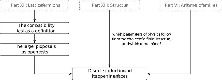
Which declared group, representation, selector and comparison fit together, and which proposed correspondences are still missing? A finite symmetry can act on a spinor, on a rotation space, or on values at the vertices. Those actions are different data.
The test uses the representation datum, the binary tetrahedral quotient and its two fibers, the central idempotent of the real group algebra of \(2T\), and the separation of spinor and internal factors in the covariant Dirac operator. The identities proved here do not use the structure questions.
A compatibility datum names the group, the coefficient field, the representation, the action on the finite graph, the selector and one reference comparison. Then 5 criteria say what has been proved, what is only conditional, and what is open. The worked case is the binary tetrahedral spinor. Correspondences for the larger classical groups are not constructed. They are recorded as open tests.
Definition 40.1. A five-part compatibility datum [fdip-009Z]AGENTDRAFTED
- November 2, 2026
Definition 40.1. A five-part compatibility datum [fdip-009Z]AGENTDRAFTED
- November 2, 2026
A compatibility datum is a tuple \[(G,\mathbb K,\rho ,\alpha ,\sigma ,C).\] Here \(G\) is a group, \(\mathbb K\in \{\mathbb R,\mathbb C\}\) is its coefficient field, and \(\rho :G\to GL_{\mathbb K}(F)\) is a finite-dimensional representation on a fiber \(F\). The map \(\alpha \) is an action of \(G\) on a finite graph substrate, in the sense of a representation datum. The selector \(\sigma \) is an idempotent in a declared algebra of operators on \(F\), or on a finite direct sum of such fibers. The reference comparison \(C\) is a stated homomorphism, quotient, or numerical identification against one named object. The coefficient field is scalar data for \(F\). It is not a residual gauge group. When \(\mathbb K=\mathbb R\), a complex representation enters only after realification, as a real representation on the underlying real vector space. A direct sum of that real fiber with another real fiber is then one real representation.
The datum is tested against 5 criteria.
- Exactness. The group, the field, the representation and the substrate action are all specified. An inclusion into a matrix group is not a substitute for the missing slot.
- Declared maps. Each comparison with a Dirac, Lorentz, gauge or gravitational structure names the homomorphism, kernel, cover or branching rule that is actually used.
- Separation. A spinor or Dirac action is identified with a gravitational action only when a separate compatibility law is proved. Sharing a name, or an inclusion into \(SU(2)\), is not that law.
- Selector effect. The selector is given, and there is a proof of the change it makes to the operator or parameter named in the datum.
- Reference recovery. The comparison names the ordinary object recovered in the chosen reference sector, or it records that the datum claims no such recovery.
For a fixed datum, each criterion is marked proved, conditional or open. Proved means the finite obligation stated in that criterion is established. Conditional means a stated part is established and the complementary part is unresolved. Open means the required map or recovery is not constructed. An open mark records that absence. It is not a theorem that no later construction exists.
Proposition 40.2. Finite identities for the binary tetrahedral spinor [fdip-00A0]AGENTDRAFTED
- November 2, 2026
Proposition 40.2. Finite identities for the binary tetrahedral spinor [fdip-00A0]AGENTDRAFTED
- November 2, 2026
Let \(2T\) be the group of 24 Hurwitz units in the binary tetrahedral quotient. In this model the central group element is the quaternion \(-1\). The distinguished central involution of the abstract group is the preimage of that quaternion under the comparison isomorphism, not the quaternion itself. Let \(\pi :SU(2)\to SO(3)\) be the conjugation homomorphism of Proposition 30.8, and write \(R_T=\pi (2T)\). Let \(\rho _s\) be the defining representation on \(\mathbb C^2\) through the matrix map \(M\) of the same statement, and let \(\tau \) be the three-dimensional representation on \(\operatorname {span}_{\mathbb R}\{i,j,k\}\) given by \(\tau (q)v=qvq^{-1}\). Both are the fibers of the two-fiber example. The substrate action \(\alpha \) is trivial. On the sum \(F=\mathbb C^2\oplus \mathbb R^3\), with \(\rho =\rho _s\oplus \tau \), the selector \(\sigma \) of the compatibility datum is the idempotent \[P=\frac {I-\rho (-1)}2.\] The abstract involution \(z\) maps to the quaternion \(-1\), so \(P\) is the image of the central idempotent \(e_-=(1_A-[z])/2\) under \(\rho \). That idempotent is the one in the real group algebra. The reference comparison \(C\) is the pair of homomorphisms \(\pi :SU(2)\to SO(3)\) and the vertex identification \(R_T\cong A_4\) proved below.
Then \(\ker (\pi |_{2T})=\{1,-1\}\), the vertex action induces \(R_T\cong A_4\), and \[P=I_2\oplus 0.\] Left multiplication by the quaternion \(-1\) is \(-1\) on the quaternion module, so that module is fixed by \(e_-\) and annihilated by \(e_+=(1_A+[z])/2\). The products of the \(d=3\) Clifford matrices of the spatial Dirac operator reproduce the quaternion multiplication table. None of these identities supplies a covariance law for that Dirac operator.
Proof.
- November 2, 2026
Proof.
- November 2, 2026
The kernel statement is the restriction of \(\ker \pi =\{1,-1\}\) from Proposition 30.8. The same source identifies \(2T\) with the full preimage \(\pi ^{-1}(R_T)\) and gives \(|R_T|=12\). The matrix \(M(-1)=-I_2\), so \(\rho _s(-1)=-I_2\). Conjugation by the quaternion \(-1\) is the identity, so \(\tau (-1)=I_3\). Therefore \[P=I_2\oplus 0.\] On the quaternion module, left multiplication by the quaternion \(-1\) is \(-1\), so that module's algebra action sends \(e_-\) to \(1\) and \(e_+\) to \(0\). The abstract involution maps to that quaternion, and \(\rho =\rho _s\oplus \tau \), so \[\rho (z)=-I_2\oplus I_3.\] Hence \(\rho (e_-)=(I-\rho (z))/2=P\), while \[\rho (e_+)=(I+\rho (z))/2=0\oplus I_3.\] The scalar \(0\) is the quaternion-module action of \(e_+\), not this operator.
Label the 4 imaginary vectors of Proposition 30.8 by \[v_1=(1,1,1),\; v_2=(1,-1,-1),\; v_3=(-1,1,-1),\; v_4=(-1,-1,1).\] Their differences \[v_2-v_1=(0,-2,-2),\; v_3-v_1=(-2,0,-2),\; v_4-v_1=(-2,-2,0)\] are linearly independent: after removing the common factor \(-2\), the determinant of \[\begin {pmatrix}0&1&1\\1&0&1\\1&1&0\end {pmatrix}\] equals \(2\). A rotation fixing all 4 vertices therefore fixes a basis of \(\mathbb R^3\) and is the identity. The vertex action gives an injective homomorphism \(R_T\to S_4\).
Conjugation by \(i\) is the coordinate map \((x,y,z)\mapsto (x,-y,-z)\). Indeed, for \(v=xi+yj+zk\), \[iv=(-x)+(yk-zj),\qquad (iv)(-i)=xi-yj-zk,\] where the last step uses \(ji=-k\) and \(ki=j\). The same expansion with cycled units gives \[j:(x,y,z)\mapsto (-x,y,-z),\qquad k:(x,y,z)\mapsto (-x,-y,z).\] On the 4 vertices these are the permutations \[(1\;2)(3\;4),\qquad (1\;3)(2\;4),\qquad (1\;4)(2\;3).\] Each is even. Let \(u=-1+i+j+k\) and \(\omega =u/2\in 2T\). Direct multiplication yields \[\begin {array}{c|c} v&uv\overline u/4\\\hline v_1&v_1\\ v_2&v_4\\ v_3&v_2\\ v_4&v_3 \end {array}\] so \(\pi (\omega )\) fixes \(v_1\) and acts by the cycle \((2\;4\;3)\). This cycle is even. Conjugation by it permutes the three double transpositions: \[\begin {aligned} (2\;4\;3)(1\;2)(3\;4)(2\;4\;3)^{-1}&=(1\;4)(2\;3),\\ (2\;4\;3)(1\;4)(2\;3)(2\;4\;3)^{-1}&=(1\;3)(2\;4),\\ (2\;4\;3)(1\;3)(2\;4)(2\;4\;3)^{-1}&=(1\;2)(3\;4). \end {aligned}\] The cycle has order \(3\), while every non-identity element of that Klein subgroup has order \(2\), so the two subgroups meet only at the identity. These 12 permutations are the vertex permutations of products in \(R_T\). They are distinct, and \(|R_T|=12\), so they exhaust the vertex image. All 12 are even. Combined with injectivity, the vertex map is an isomorphism \(R_T\cong A_4\). The composite \(2T\to R_T\to A_4\) has kernel \(\{1,-1\}\).
For the \(d=3\) matrices of Definition 16.1, \(\gamma _a^2=I\) and \(\gamma _a\gamma _b=-\gamma _b\gamma _a\) whenever \(a\ne b\). Set \[I\mapsto 1,\quad \gamma _1\gamma _2\mapsto i,\quad \gamma _2\gamma _3\mapsto j,\quad \gamma _1\gamma _3\mapsto k.\] Then \[(\gamma _1\gamma _2)^2=-\gamma _1^2\gamma _2^2=-I,\] and the same sign occurs for the other two products. Also \[(\gamma _1\gamma _2)(\gamma _2\gamma _3)=\gamma _1\gamma _3,\] and the two cyclic products match \(jk=i\) and \(ki=j\). These are the quaternion relations. They identify an action of the same abstract group on the even products. They do not state an intertwiner between left multiplication and the spatial operator \(\sum _j\gamma _j\nabla _j\).
Proposition 40.3. Status of the five criteria [fdip-00A1]AGENTDRAFTED
- November 2, 2026
Proposition 40.3. Status of the five criteria [fdip-00A1]AGENTDRAFTED
- November 2, 2026
For the binary tetrahedral datum of the finite spinor identities, the 5 criteria of the compatibility datum have the following status. Exactness, the selector effect and reference recovery are proved. The declared maps and the spinor separation are conditional. The unresolved part of the declared maps is the absence of the larger classical correspondences. That absence is not a nonexistence theorem.
The worked test in the background plan was left multiplication of \(2T\) on the spinor module \(\mathbb H\) of \(Cl^+(3)\). The test published in Proposition 40.2 is \(\rho _s\oplus \tau \) on \(\mathbb C^2\oplus \mathbb R^3\). Left multiplication on \(\mathbb H\cong \mathbb R^4\) is the realification of \(\rho _s\). The rotation summand \(\tau \) is additional.
Proof.
- November 2, 2026
Proof.
- November 2, 2026
Exactness is proved. The group is the Hurwitz model of \(2T\), and the coefficient field is \(\mathbb R\). The spinor fiber \(\mathbb C^2\) is realified as \(\mathbb R^4\), and the rotation fiber is \(\mathbb R^3\), so \(T(g)=\rho _s^{\mathbb R}(g)\oplus \tau (g)\) lies in \(GL_7(\mathbb R)\). Realification carries \(\rho _s(-1)=-I_2\) to \(-I_4\), and \(\tau (-1)=I_3\), so \(T(-1)=-I_4\oplus I_3\). The complex block form \(P=I_2\oplus 0\) in Proposition 40.2 realifies to \(I_4\oplus 0\). The graph action is the trivial action declared with these representations.
The declared maps are conditional. The two maps that are constructed are \(\pi :SU(2)\to SO(3)\) with kernel \(\{1,-1\}\), and \(2T\to A_4\) with the same kernel. Both are the finite identities of Proposition 40.2. No homomorphism, kernel, cover or branching rule is constructed here for \(Sp(3,1)\), \(SU(3,1)\), \(SU(3,2)\), \(SL(4,\mathbb R)\), or a Hessian extension. Those comparisons remain open. Their absence is not a nonexistence theorem.
Separation is conditional. The spinor representation sends the quaternion \(-1\) to \(-I_2\), while the rotation representation sends it to \(I_3\). The representation datum already separates an internal factor \(1\otimes \rho \) from an action on the spinor factor, and the covariant Dirac operator requires Clifford compatibility before a binary rotation group can act as a gauge transformation. The quaternion multiplication table of Proposition 40.2 does not provide that compatibility law. The gravitational comparison available here is only the quotient \(SU(2)\to SO(3)\). A larger gravitational identification is unresolved.
The selector effect is proved for the operator named in the datum. With \(P=I_4\oplus 0\) the realified selector, \[PT(g)P=\rho _s^{\mathbb R}(g)\oplus 0.\] This is the block identity for that projection: it retains the realified spinor block and removes the rotation block. The same idempotent is not a link variable of the covariant Dirac operator, so this identity makes no claim about the kernel of that operator.
Reference recovery is proved for the declared comparison \(C\). That comparison is \(\tau :2T\to A_4\subset SO(3)\), the tetrahedral rotation representation. The kernel is \(\{1,-1\}\) and the image has order \(12\), as proved in Proposition 40.2. The spinor fiber does not factor through that quotient. That caveat is stated under separation, above. It does not leave the recovery of this rotation representation unproved. The datum claims no lattice measure, continuum quantum field, or laboratory observable beyond this finite rotation representation.
41. The larger proposals as open tests [fdip-00A2]AGENTDRAFTED
- November 2, 2026
41. The larger proposals as open tests [fdip-00A2]AGENTDRAFTED
- November 2, 2026
The compatibility test fixes one finite spinor datum. The same 5 criteria now record the larger proposals left open by the status of that datum. Each proposal states the claim under test, the algebraic datum already in hand, the map that is missing, and whether any finite witness is available. An open mark records that absence. It is not a theorem that no later construction exists, and it is not a physical identification.
The 4 Lie-group names are those already listed as unconstructed in Proposition 40.3. Their source claims are not the same. Three names do not occur in the cited Wilson paper. \(SL(4,\mathbb R)\) does, in a later section, and the Hessian route is the claim of Section 2.2. Both remarks below quote the claim that was rechecked and say what is missing. A correspondence still has to specify an action and a representation, an algebra map, any preserved structure or form, a unit-group choice where applicable, and the intended physical meaning, as required by why begin with 2T?. Resemblance is not a model, and neither remark below adopts a group.
The two remarks below keep these proposals open. Neither remark adopts a group as the symmetry of the lattice theory, and neither draws a no-go conclusion from the missing map.
Remark 41.1. Four Lie-group proposals remain open [fdip-00A3]AGENTDRAFTED
- November 2, 2026
Remark 41.1. Four Lie-group proposals remain open [fdip-00A3]AGENTDRAFTED
- November 2, 2026
The 4 names remain open tests against the compatibility datum. The claims below were checked in arXiv:2401.13000v4, the version reached by [wilson2024discrete]. The finite maps proved for the binary tetrahedral spinor are not claimed to factor through any of the 4 names.
\(Sp(3,1)\), \(SU(3,1)\) and \(SU(3,2)\) do not occur in that version. The FDIP record lists them as candidate groups mentioned while the programme was being planned. The known algebraic datum in these notes is the name alone: no dimension, real form, matrix realization, coefficient field, or action on a finite graph is fixed here. The missing map is a stated homomorphism, kernel, cover or branching rule, together with a selector and a reference object. No finite witness is supplied. All 5 criteria are open.
\(SL(4,\mathbb R)\) is named by Wilson. In Section 6.8, page 23, three rows of products of generators drawn from two copies of \(Q_8\) extend \(SO(4)\) to \(SL(4,\mathbb R)\) [wilson2024discrete, v4, Section 6.8, p. 23]. He gives two interpretations of that group: as a double cover of \(SO(3,3)\), and so as a symmetry of a six-dimensional spacetime, or as three directions of momentum and three of angular momentum inside a four-dimensional spacetime. He writes that this breaks the identification of \(SL(2,\mathbb C)\) with \(SO(3,1)\), so that the two become disjoint subgroups of \(SL(4,\mathbb R)\), and that the gain would be a generally covariant reading of the Standard Model. Section 7.3, page 25, later says that 4 quaternionic coordinates are acted on by \(SL(4,\mathbb R)\) as spacetime symmetries. The known datum here is that pair of sentences. No matrix realization on a finite graph, selector, or reference comparison is constructed in these notes. All 5 criteria are open. The open mark does not assert that a later realization is impossible.
Remark 41.2. The Hessian route remains an open test [fdip-00A4]AGENTDRAFTED
- November 2, 2026
Remark 41.2. The Hessian route remains an open test [fdip-00A4]AGENTDRAFTED
- November 2, 2026
The Hessian proposal is the route recorded in the Hessian-group outlook. That remark begins with \[Q_8\rtimes C_3\cong 2T\] and then names the iterated semidirect product \((G_{27}\rtimes Q_8)\rtimes C_3\). The actions in those products are part of the data. The name of the product does not choose them. The same remark states that a central scalar subgroup \(C_3\leq G_{27}\) has quotient the Hessian group of order 216, and that the larger group is a triple cover of that quotient. This chapter does not reconstruct \(G_{27}\), the semidirect actions, or that quotient.
The source sentence was rechecked in arXiv:2401.13000v4. Section 2.2 is page 5 of that file [wilson2024discrete, v4, Section 2.2, p. 5]. The locator pages 4 to 5 in Remark [fgap-001X] do not match this version. On page 5 Wilson states that the matrices for \(G_{27}\) and \(Q_8\) generate a group of order 216, the semidirect product \(G_{27}\rtimes Q_8\), and that the full group has order 648 and is the triple cover of the Hessian group. He writes that it can be interpreted as a finite analogue of \(U(1)\times SU(2)\times SU(3)\), and that the finite group is the iterated semidirect product \(G_{27}\rtimes Q_8\rtimes Z_3\). The cyclic factor of order 3 is the group written \(C_3\) in the display above. These notes record the interpretation and do not adopt it.
The known algebraic datum is the binary tetrahedral group already used in the finite spinor identities. The displays \(Q_8\rtimes C_3\cong 2T\) and \((G_{27}\rtimes Q_8)\rtimes C_3\) are not presentations and are not further data: their actions are not chosen, and neither \(G_{27}\) nor the order-216 quotient is constructed here. The missing map is a typed homomorphism from the iterated product, or from its order-216 quotient, into \(U(1)\times SU(2)\times SU(3)\) or into a group already constructed in these notes. The comparison with \(U(1)\times SU(2)\times SU(3)\) stays an attributed proposal in Remark [fgap-001X]. It is not an isomorphism, and the comparison motivation recorded beside that outlook is not a construction of the finite group.
The finite witness available now is \(2T\) alone. It does not determine \(G_{27}\) or the order-216 quotient. A witness that would meet the compatibility datum would specify one of those groups by a concrete model, a coefficient field, a representation on a named fiber, an action on a named finite graph, a selector, and one reference comparison. None of those slots is filled, and a matrix model would not by itself fill the missing action. Every criterion is open. That absence is not a no-go theorem and not a physical identification.
42. Discrete induction and its open interfaces [fdip-003W]AGENTDRAFTED
- November 3, 2026
42. Discrete induction and its open interfaces [fdip-003W]AGENTDRAFTED
- November 3, 2026
How can algebra and geometry organize induction and background variation? Gaussian elimination gives a finite example; the synthesis conjecture and finite interfaces distinguish this result from the further maps required.
The route through these explorations is the diagram opening the compatibility test. That test fixes one finite spinor datum. The larger proposals remain open tests. The conjecture and finite interfaces below remain distinct from those open questions.
The constructions now on this route include finite-group symmetry, selected backgrounds and connections, finite and compact gauge fields, reflection positivity, explicit transfer operators, Gauss's law, Grassmann integration, fermionic elimination, the covariant Dirac operator and the free Wilson remedy. The arrow from gauge fields to Euclidean time, drawn in the reader guide, is a reading prerequisite for the gauge transfer and for Gauss's law. Reflection positivity alone does not supply that time shift. The arrow from gauge fields to lattice fermions is a reading prerequisite for the covariant Dirac operator and for the free Wilson remedy that follows it, not for Grassmann integration or fermionic elimination, and not an identification of those operators with a physical electron.
The comparisons that remain open are these. The physical environment map \(E\) is not constructed. The supplied-circle limit controls one fixed Fourier mode; it is not a continuum limit of the full induced law, and no moduli map controls that limit. The enriched background groupoid and the geometric realization do not supply a site, a stack, or a descent that organizes those families. The larger proposals remain open tests. What the structure fixes and what it leaves free records that comparison. The chapters transcluded by Structure develop the questions of that part. None of these absences is a no-go theorem or a physical identification.
Wilson's claims. The tested claims are the two finite maps of Proposition 40.2: conjugation \(SU(2)\to SO(3)\) and the quotient \(2T\to A_4\), both with kernel \(\{1,-1\}\). The larger proposals in § 41 stay open. Three of the 4 Lie names do not occur in the cited Wilson paper, and the Hessian and \(SL(4,\mathbb R)\) claims are recorded there as interpretations. The absence of a construction is not a no-go theorem and not a physical identification.
Next questions. What remains can be stated as 4 questions. The physical environment map \(E\) is still unconstructed. The continuum comparison is still the one fixed Fourier mode of Proposition 20.1.3. The higher-dimensional area law, fermion reflection positivity and fermion transfer, and infinite-volume reconstruction were not proved. Whether continuous space comes back at large scales, without being supplied, is left to a separate plan; § 42.2 asks it and does not answer it. The enriched background groupoid and the geometric realization still do not supply a site, a stack, or a descent. Whether the context square organises the selectors remains open, and no stack is proved. Wilson's finite maps are tested, and the larger proposals remain open tests.
42.1. The conjecture and its finite evidence [fdip-009H]AGENTDRAFTED
- November 1, 2026
42.1. The conjecture and its finite evidence [fdip-009H]AGENTDRAFTED
- November 1, 2026
The synthesis conjecture proposes a wider theory. The finite evidence separates the constructions already established from their open interfaces.
Conjecture 42.1.1. A discrete induced arithmetic theory [fdip-003X]AGENTDRAFTED
- October 30, 2026
Conjecture 42.1.1. A discrete induced arithmetic theory [fdip-003X]AGENTDRAFTED
- October 30, 2026
The discrete induced theory is an arithmetic scheme equipped with a Clifford sheaf and a finite group action; the continuum limit and the background dependence are controlled by a map from a moduli stack; the numerical parameters of the resulting QFT are special values of L-functions attached to the arithmetic data.
This is a schematic research conjecture. An arithmetic family of forms, its Clifford algebra sheaf and a specified finite-group action are available finite constructions. The moduli-stack clause is an informal target for organizing families, isomorphisms and descent; no site, stack or continuum comparison map has been specified here. Nor has an arithmetic L-function or its special value been identified with a parameter of a quantum field theory (QFT). These terms describe the conjectured interfaces, not additional structures carried by every finite Gaussian model.
The first background-selection question is algebraic. Schematically, let \(B_{\mathrm {alg}}\) denote a chosen set of algebraic background data and \(\mathcal S\) a chosen set of admissible structures; a selector would be a map \[\sigma :B_{\mathrm {alg}}\longrightarrow \mathcal S.\] A physical interpretation would additionally require a set \(\operatorname {Env}_{\mathrm {phys}}\) of physical environments and a map \[E:\operatorname {Env}_{\mathrm {phys}}\longrightarrow B_{\mathrm {alg}}.\] Neither map is asserted to have been constructed by the enriched-background example. The finite interfaces and their limits specify what the present calculations do establish.
Remark 42.1.2. Finite evidence for the synthesis conjecture [fdip-003Y]AGENTDRAFTED
- November 2, 2026
Remark 42.1.2. Finite evidence for the synthesis conjecture [fdip-003Y]AGENTDRAFTED
- November 2, 2026
The synthesis conjecture connects discrete induction to arithmetic, symmetry, backgrounds, continuum limits and physical observables. The opposite-vertex elimination supplies a concrete finite comparison: averaging the removed fields preserves retained expectations, while fixing those fields can change them. The following 8 comparisons distinguish such proved constructions from the additional identifications required by each part of the conjecture.
- Arithmetic scheme. The arithmetic four-cycle family gives an explicit coefficient ring and separate open domains for a nondegenerate form, an invertible eliminated block and a trace observable. The bad fibers show why these domains differ. This constructs a family; it does not select a unique arithmetic model for a physical system. The background arc adds no arithmetic scheme.
- Clifford sheaf. The configuration Clifford algebra and its form-preserving maps extend to a sheaf compatible with scalar extension. For the enriched rational objects, Schur elimination multiplies the Galois characters of the retained and eliminated even centers. Primitive Dirichlet representatives must be formed after this product; multiplying their zero extensions need not give the same function, and no L-function multiplication rule follows. A physical spin or matter interpretation and an analytic coupling to observables require further maps. Configuration Clifford algebras and spatial Clifford modules are distinct objects. Grassmann integration is a later algebraic calculus. It is not this sheaf.
- Finite-group action. The specified half-turn, group-algebra action and sector marginals make symmetry and Gaussian elimination compatible under their stated hypotheses. The cycle half-turn fixes the even Clifford center pointwise; the nontrivial algebra involution of that center is a different action. These supplied symmetries do not select a physical gauge group or its dynamics. The background arc adds the real isotypic projectors of finite-group symmetry of Gaussian fields and the finite gauge laws of the pure-gauge torus and the surface character formula. Those laws are finite-group constructions. They do not choose a physical gauge group either.
- Backgrounds and moduli. The enriched background groupoid specifies objects, arrows, reference pairings and retained projections. Scalar descent preserves chosen invariants, while quadratic isometry can forget essential background data. The two-vertex comparison makes a second forgetting explicit: the same unweighted interval and retained endpoint admit different Gaussian variances. A groupoid of this kind alone supplies neither descent over a site nor a physical environment-selection map. Selected backgrounds and connections, from § 22 through § 25, keep that limit: a connection there is a fixed background, and the joint matter law of Example 29.4 does not supply a site or a stack.
- Continuum comparison. The finite spatial Dirac calculation and its zero modes and nearest-neighbor comparison identify finite spectra and an operator mismatch. The supplied-circle limit now proves convergence of one fixed Fourier mode, its massive inverse and its Gaussian second moment. This is not convergence of the full induced law or a map from moduli controlling a continuum limit. The background arc does not extend this comparison. Its finite transfer operator Theorem 32.2, the reflection counterexample Example 31.4, and the free Wilson kernel Theorem 38.2 remain finite-volume statements.
- Parameters and L-values. The trace ratio is an independently defined finite observable; its cycle values distinguish backgrounds. Two rational fibers are isometric as quadratic forms but have different trace ratios. The fiber-constancy criterion therefore excludes recovering this ratio from the rational quadratic-isometry class, and hence from its Clifford algebra, center character or any fixed collection of character-only L-values. No physical parameter is identified; arithmetic data that also retain the reference pairing and mass remain outside this obstruction. The background arc adds no L-value.
- Discrete induction. The Gaussian elimination theorem, retained expectation and cycle calculation construct an effective precision, normalization factor and new couplings, with symmetry transport. A formal quartic interaction composes under elimination through second order in its coupling and transports a supplied symmetry. The three-coordinate example exhibits constant, quadratic, quartic and sextic terms and computes a normalized connected four-point function; stationary elimination separates tree contributions from fluctuation terms. These finite formal calculations do not reconstruct eliminated data or supply a nonperturbative theory. The background arc adds the rooted-forest expansion Theorem 23.5, the interacting selected background, and fermionic elimination, each at the scope stated in those notes.
- Physical equations and observables. These finite operators and normalized laws form a mathematical foundation. A comparison with Standard Model, quantum-field or general-relativistic equations still requires specified dynamics and observables, including the relevant gauge, matter, time and gravitational structures. No such physical identification is established by the finite identities above. The binary-tetrahedral test Proposition 40.2 adds two finite homomorphisms and no laboratory observable. The Hermitian Wilson counterexample Example 38.3 is a convention check, not an identification.
42.2. What the structure fixes and what it leaves free [fdip-009G]AGENTDRAFTED
- November 3, 2026
42.2. What the structure fixes and what it leaves free [fdip-009G]AGENTDRAFTED
- November 3, 2026
Which features follow from a chosen finite structure, and which remain additional inputs?
Part VII compared the discrete physics with a continuous space that was supplied. The supplied-circle limit controls one fixed Fourier mode. Part XIII has since built cochains and their Hodge theory, a distance read from a commutator, and exact coarse-graining of a hierarchical precision. Whether the physics of continuous space comes back at large scales without being supplied can now be asked. Its answer is left to a separate plan. This section does not answer it, and it draws no continuum limit.
Wilson's finite groups stay first. The tested claims are the two finite maps of Proposition 40.2: conjugation \(SU(2)\to SO(3)\) and the quotient \(2T\to A_4\), both with kernel \(\{1,-1\}\). Those maps fix the named kernels. The larger proposals remain open tests. The absence of a construction is not a no-go theorem and not a physical identification.
Several programmes outside this forest have not been read: a spectral derivation of the Standard Model, causal sets, loop quantum gravity, and the string landscape. This note does not record what they fix or leave free.
The Euler product, for \(\operatorname {Re}s>1\), is the product over primes not dividing \(2\det Q\) of \(\,(1-\hat Z_p(Q)\,p^{-s})^{-1}\). It equals \(L(s,\chi _D)\) times the product, over primes dividing \(2\det Q\) but not \(D\), of \(\,(1-\chi _D(p)\,p^{-s})\). The Gaussian induced action takes the weight to be half the logarithm of a determinant. The cycle scaling sends \((\log \det Q_n)/2-n\log n\) to a limit on the cycle. These are not the same object. This note does not identify the Euler product with that logarithm or with that limit.
The operator-algebra notes replace a supplied conditional expectation by the composition law for nested expectations (Theorem 39.1.2), and they replace a supplied fixed-point algebra by the image of the average (Theorem 39.2.2). The crossing block sets the reflection rank (Theorem 39.2.1). None of these is a continuum reconstruction.
On every square torus the Betti numbers are \((1,2,1)\) (Theorem 39.3.1), and the harmonic cochains realize them (Theorem 39.3.2). The ordered compositions of exterior multiplication and contraction span the endomorphisms of the exterior algebra (Theorem 39.4.1). The cup product obeys the graded Leibniz rule and is not graded-commutative on cochains (Theorem 39.4.2). The note does not claim that the resulting Clifford representation is injective.
The Connes distance is computed on the stated finite triples (Theorem 39.5.1). The edge-source triple makes the distance the graph distance when each vertex has at most one incoming edge, and on one grid it lies strictly between the Euclidean distance and the graph distance (Theorem 39.5.2). On a triangle-free graph the gauge-dependent part of the fourth power of the massless covariant Laplacian is 8 times the sum of \(\cos \varphi _c-1\) over the undirected 4-cycles (Theorem [fdip-00A7]). The comparison of that trace with the logarithm of a massive determinant remains speculative. Neither finite trace is identified with a continuum limit.
Nested residue classes diagonalize a hierarchical precision (Theorem 39.7.1). Block means of that precision keep a hierarchical second-moment matrix (Theorem 39.7.2). For geometric coefficients, relevance of the top coefficient holds only for \(0<\lambda <1\). A hierarchical Gaussian has site fourth moment \(3\sigma ^4\) (Theorem 39.7.3). No non-Gaussian hierarchical fixed point is proved. These matrix relations do not by themselves produce a Gaussian measure on functions on the \(p\)-adic integers.
Surface gluing of the finite-group state sum is convolution of class functions (Theorem 39.8.1). That convolution is not identified with the spatial transfer operator. On a finite incidence presentation, invariant tensors count the gauge orbits (Theorem 39.8.2). One square in \(M_4(\mathbb C)\) cuts out 6 contexts with no global point, while each context separately has a character (Theorem 39.9.1). Whether that obstruction organises the selectors remains open (§ 39.9). Subgroup action groupoids form a groupoid-valued presheaf on the opposite of the subgroup poset (Theorem 39.9.2). No stack is proved.