Let \(G=(V,E,s,h)\) be a finite incidence presentation. Its one-dimensional realization is the quotient space \[|G|=\bigl (V\sqcup (E\times [0,1])\bigr )/{\sim },\] where \(V,E\) are discrete, the intervals have their usual topology, and the equivalence relation is generated by \[(e,0)\sim s(e),\qquad (e,1)\sim h(e).\] Use the quotient topology. Thus each vertex is a point and each edge supplies an open interval attached at its endpoints, the standard one-dimensional CW construction of [hatcher2002algebraic, Section 1.A, p. 83]. Loops have both endpoints attached at one vertex; parallel edges remain separate intervals. Direction chooses the parametrization from \(0\) to \(1\), not a causal ordering.

Declare a morphism \(f:G\to G'\) to be a pair of maps \(f_V:V\to V'\) and \(f_E:E\to E'\) with \[f_Vs=s'f_E,\qquad f_Vh=h'f_E.\] It induces \[\begin {aligned} |f|:|G|&\longrightarrow |G'|,\\ [v]&\longmapsto [f_V(v)],\\ [e,t]&\longmapsto [f_E(e),t]. \end {aligned}\] These formulas respect the endpoint identifications. They are continuous before quotienting, so the quotient topology makes \(|f|\) continuous. Identity and composition follow from the formulas. This proves functoriality for these declared incidence maps; arbitrary edge contractions have not been included among them. The map construction is a direct deduction from the quoted quotient model.

Take the simple undirected triangle on vertices \(\{0,1,2\}\). Give its three edges any orientations, then forget them here; any parallel copies would also have to be merged before this simple undirected comparison. The one-dimensional realization retains the three edges without a face. In the nonempty-face convention of [maypishevar2025finitespaces, Definition 6.1.1, p. 61], its boundary complex and the filled complex have faces \[\begin {aligned} K_{\partial } &=\{\{0\},\{1\},\{2\},\{0,1\},\{1,2\},\{0,2\}\},\\ K_{\Delta }&=K_{\partial }\cup \{\{0,1,2\}\}. \end {aligned}\] The added face consists of three pairwise adjacent vertices: it is the filled clique triangle. This specifies these two complexes, without declaring a general clique-construction functor.

Choose three noncollinear points \(v_0,v_1,v_2\) in the plane. Realize each listed face by the convex hull of its vertices, as in [maypishevar2025finitespaces, Definitions 6.2.1 and 6.2.6, pp. 62-63]. Then \(|K_{\partial }|\) is the perimeter and \(|K_{\Delta }|\) is the closed triangular region. Traversing the three line segments identifies the perimeter with \([0,3]/(0\sim 3)\): the induced map is a continuous bijection from a compact space to a Hausdorff space, hence a homeomorphism. The map \(t\mapsto \exp (2\pi i t/3)\) gives the same identification with \(S^1\).

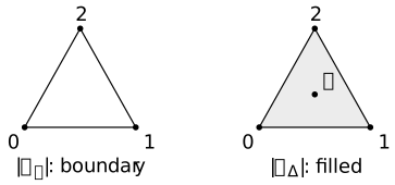
The filled triangle contracts to its barycenter \(b=(v_0+v_1+v_2)/3\) by \[H(x,t)=(1-t)x+tb,\qquad 0\leq t\leq 1.\] Convexity keeps \(H(x,t)\) in the triangle, and the formula is continuous, with \(H(x,0)=x\) and \(H(x,1)=b\). The two constructions have the same vertices and edges, but only the second supplies a two-dimensional face. Incidence alone therefore does not choose between keeping the perimeter and filling it. Each specified realization is nevertheless a well-defined construction.

These comparisons are elementary deductions from the cited realization definitions. Mathlib's AbstractSimplicialComplex uses nonempty faces and includes each vertex; its Convex.contractibleSpace supplies contractibility of a nonempty convex subset of a real topological vector space. These support the conventions and the contraction step, not the complete incidence-to-triangle comparison.

For each \(w>0\), let \(\mathcal B_w\) be the finite Gaussian background with vertices \(V=\{0,1\}\), one edge \(0\to 1\) of weight \(w\), counting pairing, mass \(m=1\), retained set \(R=\{0\}\) and eliminated set \(V\setminus R=\{1\}\). The field coordinates remain labelled. The weighted Laplacian and massive precision are \[\begin {aligned} L_w&=w\begin {pmatrix}1&-1\\-1&1\end {pmatrix},\\ Q_w&=I+L_w=\begin {pmatrix}1+w&-w\\-w&1+w\end {pmatrix}. \end {aligned}\] Indeed the incidence row is \((-1,1)\). The vectors \((1,1)\) and \((1,-1)\) have precision eigenvalues \(1\) and \(1+2w\), so \(Q_w>0\). The normalized Gaussian law is therefore well-defined on counting-coordinate volume \(df_0\,df_1\), with \[\begin {aligned} d\mu _w(f)&=Z_w^{-1}\exp (-f^TQ_wf/2)\,df_0\,df_1,\\ Z_w&=\frac {2\pi }{\sqrt {1+2w}}. \end {aligned}\] The normalizer is the two-dimensional specialization of positive Gaussian normalization.

Let \(X=\{\mathcal B_w:w>0\}\) and let \(Y=\{U\}\) be the singleton whose element is the unweighted labelled directed edge \(0\to 1\) with distinguished endpoint \(0\). Define \[\begin {aligned} c:X&\longrightarrow Y,&c(\mathcal B_w)&=U,\\ r:X&\longrightarrow \mathbb R,&r(\mathcal B_w)&=\int f_0^2\,d\mu _w(f). \end {aligned}\] Thus \(c\) forgets the varying weight while retaining the labels, orientation and selected endpoint; the mass and reference pairing are fixed throughout the family. The observable is integrable by Gaussian polynomial integrability. The coordinate has zero mean, so \(r\) is the variance at the retained endpoint. Composing \(c\) with the interval realization gives the same labelled interval with that endpoint for every \(w\).

For the two-vertex family, eliminate the coordinate at vertex \(1\). The positive Schur formula and retained covariance give \[\begin {aligned} S_w&=(1+w)-\frac {w^2}{1+w} =\frac {1+2w}{1+w}>0,\\ r(\mathcal B_w)&=S_w^{-1}=\frac {1+w}{1+2w}. \end {aligned}\] In particular, \[r(\mathcal B_1)=\frac 23\ne \frac 35=r(\mathcal B_2), \qquad c(\mathcal B_1)=c(\mathcal B_2)=U.\] The fiber-constancy criterion excludes a function \(F:c(X)\to \mathbb R\) satisfying \(r=F\circ c\), even on a restricted family containing these two backgrounds. Consequently the unweighted interval with its retained endpoint also cannot recover this variance on that family. This is an obstruction for the specified forgetting and observable, not for every geometric realization.

This two-coordinate calculation is a teaching variant of the weighted-cycle comparison, which already gives unequal retained correlations \(2/15\) and \(16/105\) at fixed mass and fixed retained pair. The same principle is visible with one retained coordinate: incidence and the selected endpoint do not retain the weighted precision. By contrast, weight-preserving relabelings, with the retained projection and observable transported together, preserve expectations by Gaussian transport. Enlarging their comparison to forget weights need not preserve them.

The retained-variance example tests scalar factorization: for specified functions \(c:X\to Y\) and \(r:X\to \mathbb R\), it asks whether \(r=F\circ c\) for a function on \(c(X)\). The fiber criterion answers exactly this question, without supplying continuity or any categorical structure.

Functorial factorization instead starts with categories and functors \(U:\mathcal B\to \mathcal D\) and \(O:\mathcal B\to \mathcal A\), and asks for \(\overline O:\mathcal D\to \mathcal A\) and a natural isomorphism \(O\cong \overline O\circ U\). A localization at a declared class \(W\) of arrows has an additional universal property: it inverts those arrows and is universal among functors that do so [stacks2017stacks, Section 4.27], Tag 04VB. A generic forgetful functor is not thereby a localization. Mathlib's CategoryTheory.Localization.lift requires both a localization functor and a functor that inverts \(W\); these hypotheses are absent from the scalar example.

Local-to-global descent requires a site with covers, restriction maps and compatible data on overlaps, together with an effective gluing statement. For category-valued data, a stack also requires a fibred category and sheaves of morphisms [stacks2017stacks, Definition 8.4.1], Tag 0268. The enriched background groupoid and the scalar variance calculation supply none of this cover-and-gluing structure. The groupoid is a category of finite backgrounds, not necessarily a finite category. No local-to-global descent theorem follows.