Example. Fourier modes and their Gaussian moments on a circle mesh [fdip-004I]
AGENTDRAFTED
For the circle mesh, let \(k\in \mathbb Z\) and set
\[e_k(x)=e^{2\pi ikx},\qquad e_{n,k}(j)=e^{2\pi ikj/n}.\]
Every entry has modulus one, hence \(\|e_{n,k}\|_n=1\). Applying
the shift and its inverse directly gives
\[\begin {aligned}
T_ne_{n,k}&=e^{2\pi ik/n}e_{n,k},\\
L_ne_{n,k}&=\lambda _{n,k}e_{n,k},\\
\lambda _{n,k}
&=n^2(2-e^{2\pi ik/n}-e^{-2\pi ik/n})\\
&=4n^2\sin ^2(\pi k/n).
\end {aligned}\]
This derives the scaled version of the
nearest-neighbor symbol. Frequencies differing by \(n\)
give the same samples. For fixed \(k\ne 0\), the condition \(n>2|k|\)
separates \(k\) from \(-k\) modulo \(n\).
For \(k=0\), \(e_{n,0}=\mathbf 1\) and \(\lambda _{n,0}=0\).
For \(k=1\), a four-point mesh has \(\lambda _{4,1}=32\); an eight-point
mesh has \(\lambda _{8,1}=64(2-\sqrt 2)\). The picture shows the supplied
unit circle sampled at 4 equally spaced points. Its arrows indicate
increasing \(j\); they do not specify a dynamics.
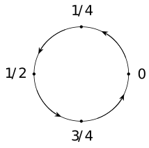
Now use real fields and the Gaussian law
\[d\nu _n(f)=Z_n^{-1}e^{-q_n(f)/2}\,d\operatorname {vol}_{g_{0,n}}(f).\]
In raw coordinates the volume and normalization are
\[\begin {aligned}
d\operatorname {vol}_{g_{0,n}}&=n^{-n/2}\,df_0\cdots df_{n-1},\\
Z_n&=(2\pi )^{n/2}(\det Q_n)^{-1/2}.
\end {aligned}\]
The volume factor follows because \(f\mapsto f/\sqrt n\) is an
orthonormal chart; the partition function is
Theorem [fdip-002T]. The covariance operator relative to
\(g_{0,n}\) is \(Q_n^{-1}\) by Theorem [fdip-000B]. Since the exponent
is \(f^TQ_nf/(2n)\), the raw coordinate covariance matrix is
\(nQ_n^{-1}\).
Define the complex Fourier observable
\(a_{n,k}=n^{-1}\sum _j e^{-2\pi ikj/n}f_j\). It has zero mean.
Writing \(v=e_{n,k}\) and \(v^*\) for its conjugate transpose,
the coordinate covariance gives
\[\begin {aligned}
\mathbb E_{\nu _n}|a_{n,k}|^2
&=n^{-2}v^*(nQ_n^{-1})v\\
&=\frac 1{\mu +\lambda _{n,k}},
\end {aligned}\]
because \(v^*v=n\). All real and imaginary parts and their products
are integrable polynomials by Proposition [fdip-002W]. In particular the
real mean \(a_{n,0}\) has variance \(1/\mu \). At \(k=1\), the
four-point and eight-point second moments are respectively
\((\mu +32)^{-1}\) and \((\mu +64(2-\sqrt 2))^{-1}\).
For \(k\ne 0\) and \(n>2|k|\), put
\[\begin {aligned}
c_{n,k}&=\operatorname {Re}a_{n,k}
=\frac 1n\sum _j\cos (2\pi kj/n)f_j,\\
s_{n,k}&=-\operatorname {Im}a_{n,k}
=\frac 1n\sum _j\sin (2\pi kj/n)f_j.
\end {aligned}\]
The geometric sum \(\sum _j e^{4\pi ikj/n}=0\): its ratio is not one,
its \(n\)-th power is one, and multiplying the sum by one minus
the ratio gives zero. Taking real and imaginary parts, and using
the double-angle identities, gives normalized squared norms
\(1/2\) for both the cosine and sine vectors and their orthogonality.
Both vectors have precision eigenvalue \(\mu +\lambda _{n,k}\), so
Theorem [fdip-000B] yields
\[\operatorname {Var}(c_{n,k})=\operatorname {Var}(s_{n,k})
=\frac 1{2(\mu +\lambda _{n,k})}.\]
The coefficients of the orthogonal projection
\(A\cos (2\pi kj/n)+B\sin (2\pi kj/n)\) are \(A=2c_{n,k}\),
\(B=2s_{n,k}\). Their variances are 4 times the displayed
projection variances.
The character calculation and normalization above are direct
deductions from the cited finite operators and Gaussian results.
Mathlib's ZMod.dft uses the counting-measure forward sum;
\(a_{n,k}\) has the additional factor \(1/n\). This formal Fourier
transform is a supporting construction, not a formalization of the
mesh limit.