Elimination and retained observables [fdip-0018]
✍️sourceAGENTDRAFTED
- October 20, 2026
Elimination and retained observables [fdip-0018]
✍️sourceAGENTDRAFTED
- October 20, 2026
Eliminating selected real field values produces both a new quadratic action and a normalization factor. The prerequisites are a positive quadratic action, its normalized Gaussian law, and the reference measure and orthogonal product volume. Inverse precision first determines covariance; averaging out the discarded variables gives retained precision equal to the Schur complement \(S\), with covariance operator \(S^{-1}\) for the specified inner product.
For integrable observables of the retained variables, retained expectation agrees with original expectation after pullback. The planned states and conditional expectations chapter asks how such averaging fits a common language of observables and states. Opposite vertices of the four-cycle make the normalization and covariance explicit. The conditional kernel distinguishes fixing variables from averaging them, while singular eliminated directions explain when the integration space itself must change.
For a formal quartic perturbation, successive Gaussian eliminations agree with direct elimination through second order in the coupling. The three-coordinate example displays the generated terms and a retained connected four-point function; stationary elimination distinguishes the tree contribution from fluctuation terms.
Theorem 1. Eliminating a positive Gaussian block [fdip-000D]AGENTDRAFTED
- October 17, 2026
Theorem 1. Eliminating a positive Gaussian block [fdip-000D]AGENTDRAFTED
- October 17, 2026
Let \(E=X\mathbin \perp Y\) be a specified orthogonal sum of finite-dimensional real inner-product spaces. Write \(h_E,h_X,h_Y\) for their pairings, \(i_X,i_Y\) for inclusion and \(p_X,p_Y\) for orthogonal projection. The addition isometry is \(J(x,y)=i_Xx+i_Yy\). Use canonical Euclidean volume on uncompleted Borel sets. Then product volume gives \(J_*(\lambda _X\otimes \lambda _Y)=\lambda _E\). Zero summands are allowed; their volume is unit mass on a singleton.
Let \(Q:E\to E\) be a self-adjoint positive precision parameter. Its components for this splitting are \[\begin {aligned} A&=p_XQi_X:X\to X,\\ B&=p_XQi_Y:Y\to X,\\ C&=p_YQi_Y:Y\to Y. \end {aligned}\] The fourth component is \(p_YQi_X=B^\dagger \), where the adjoint uses the specified pairings. Both \(C\) and the effective precision, or real Schur complement, \[S=A-BC^{-1}B^\dagger :X\to X\] are positive definite and invertible. This is the real positive specialization of the split Schur map.
Put \(w_Q(z)=\exp (-h_E(z,Qz)/2)\) and \(q=\dim Y\). For every \(x\in X\), the exact fiber integral is \[\begin {aligned} I_Q(x)&=\int _Y w_Q(J(x,y))\,d\lambda _Y(y)\\ &=c_C\exp (-h_X(x,Sx)/2),\\ c_C&=\frac {(2\pi )^{q/2}}{\sqrt {\det C}}=Z_C>0. \end {aligned}\] Moreover \(\det Q=\det C\det S\). Thus elimination induces both \(S\) and a positive finite scalar \(c_C\).
Proof.
- October 17, 2026
Proof.
- October 17, 2026
Positivity under elimination applies to these real inner products. Explicitly, testing \(Q\) on \(i_Yy\) gives \(C>0\); finite dimension makes \(C\) invertible. Put \(K=C^{-1}B^\dagger \). The orthogonal congruence identity is \[\begin {aligned} &h_E(J(x,y),QJ(x,y))\\ &\quad =h_X(x,Sx)\\ &\qquad +h_Y(y+Kx,C(y+Kx)). \end {aligned}\] Indeed \(CK=B^\dagger \) and \(K^\dagger =BC^{-1}\); expansion cancels the term subtracted in \(S\). The self-adjoint inverse of \(C\) makes \(S\) self-adjoint. For \(x\ne 0\), testing on \(J(x,-Kx)\ne 0\) gives \(h_X(x,Sx)>0\).
For fixed \(x\), translation by \(Kx\) preserves reference volume. Square completion and positive Gaussian normalization therefore give \[\begin {aligned} I_Q(x)&=e^{-h_X(x,Sx)/2} \int _Y e^{-h_Y(v,Cv)/2}\,d\lambda _Y(v)\\ &=e^{-h_X(x,Sx)/2}Z_C. \end {aligned}\] This is a nonnegative integral with a positive finite prefactor; no signed Fubini interchange is needed. The same square completion shows that the stationary field is \(y_*(x)=-Kx\). Minimization alone does not evaluate the fiber integral or its scalar.
For the determinant, let \(V(x,y)=(x,y+Kx)\) and \(D(x,y)=(Sx,Cy)\) on \(X\oplus Y\). Congruence gives \(J^{-1}QJ=V^\dagger DV\). Choose bases \(e_1,\ldots ,e_p\) of \(X\) and \(f_1,\ldots ,f_q\) of \(Y\), with the same ordered concatenation in domain and codomain. In the top wedge of the images under \(V\), we have \(Ve_j=e_j+Ke_j\) and \(Vf_k=f_k\). Any term choosing some \(Ke_j\) has more than \(q\) vectors in \(Y\), so it vanishes. The remaining term is the original top wedge; hence \(\det V=1\). In orthonormal coordinates, the adjoint is the transpose and has the same determinant, by reindexing the determinant permutation sum. The direct sum \(D\) acts on the top wedge by \(\det S\det C\). Multiplicativity of this scalar and invariance under conjugation now prove \(\det Q=\det C\det S\). Empty bases give determinant one, so the argument includes zero summands.
Taking minus the logarithm of the positive fiber integral defines an exact effective action: \[\begin {aligned} \mathcal A_{\mathrm {eff}}(x) &=\tfrac 12h_X(x,Sx)-\log c_C\\ &=\tfrac 12h_X(x,Sx)+\tfrac 12\log \det C\\ &\quad -\tfrac q2\log (2\pi ). \end {aligned}\] The constant cancels from normalized retained expectations but belongs to the unnormalized weight. Rescaling the two reference volumes by \(a_X,a_Y>0\) multiplies \(c_C\) by \(a_Y\), \(Z_S\) by \(a_X\) and \(Z_Q\) by \(a_Xa_Y\); normalized laws remain unchanged. For \(Y=0\), \(c_C=1\); for \(X=0\), \(Z_S=1\). In each case the unique zero-space endomorphism is invertible and has determinant one.
For counting fields on \(V=R\sqcup U\), the delta bases identify \(X=\mathbb R^R\), \(Y=\mathbb R^U\), \(B=H\) and \(B^\dagger =H^T\). Coordinate volume splitting recovers the usual \(dx\,dy\) formula. The carrier, split, input precision and volumes are supplied; \((S,c_C)\) is induced relative to those choices. The singular-pivot boundary requires a separate argument.
[boyd2004convex, Appendix A.5.5, pp. 650-651] gives square completion with the first block as pivot. Exchanging its order to \((y,x)\) gives the present eliminated pivot \(C\).
[rasmussen2006gaussian, Appendix A.2, equation (A.4), p. 200] gives the Gaussian density with covariance as parameter. Substituting \(C^{-1}\) gives the normalizer used here. The invariant integration and determinant argument above reconstruct these ingredients with specified pairings and volume.
Mathlib's Matrix.schur_complement_eq₂₂ supports square
completion in compatible finite coordinates, with a Hermitian
invertible eliminated block. Its Matrix.det_fromBlocks₂₂
supports the determinant identity. TauCeti's
Matrix.PosDef.gaussianCondCov supports strict Schur
positivity for a real positive-definite block matrix. Despite its
conditional-covariance name, this algebraic conclusion can be applied
to the precision \(Q\). These ingredients do not supply the integral
or its reference-volume convention.
The operation is algebraic: it acts on vertex and edge sets that are supplied, and carries neither a dynamical carrier nor an effective metric, which are additional data.
Theorem 2. The retained Gaussian marginal [fdip-000E]AGENTDRAFTED
- October 17, 2026
Theorem 2. The retained Gaussian marginal [fdip-000E]AGENTDRAFTED
- October 17, 2026
Use the orthogonal sum \(E=X\mathbin \perp Y\), positive precision \(Q\), effective precision \(S\) and exact scalar \(c_C\) of Gaussian elimination. Let \(\pi =p_X:E\to X\) and let \(\mu _Q,\mu _S\) be the independently defined Gaussian probability laws. Then \[Z_Q=c_CZ_S,\qquad \pi _*\mu _Q=\mu _S.\] Thus the retained marginal law is \(\mu _S\): for every Borel \(D\subseteq X\), \(\mu _Q(\pi ^{-1}D)=\mu _S(D)\). Here pushforward assigns \(D\) the mass of its inverse image, extending the finite pushforward convention to these Borel spaces.
Every real Borel function \(F:X\to \mathbb R\) satisfies the extended nonnegative identity \[\int _E|F\circ \pi |\,d\mu _Q =\int _X|F|\,d\mu _S\ \in [0,\infty ].\] Consequently \(F\in L^1(\mu _S)\) if and only if \(F\circ \pi \in L^1(\mu _Q)\). Under these equivalent conditions, \[\int _E F\circ \pi \,d\mu _Q=\int _X F\,d\mu _S.\] We use actual Borel functions; \(L^1\) here denotes their integrable vector space. It is not asserted to be an algebra.
Proof.
- October 17, 2026
Proof.
- October 17, 2026
The projection is linear, hence continuous and Borel. The weights are continuous and nonnegative, and the orthogonal product volumes are sigma-finite. Nonnegative Tonelli and the fiber formula give \[\begin {aligned} Z_Q&=\int _X\int _Y w_Q(J(x,y))\,d\lambda _Y(y)\,d\lambda _X(x)\\ &=c_C\int _X e^{-h_X(x,Sx)/2}\,d\lambda _X(x)\\ &=c_CZ_S. \end {aligned}\] All three factors are positive and finite by normalization. This also agrees with \(\det Q=\det C\det S\).
For a Borel set \(D\), repeat Tonelli with the nonnegative factor \(\mathbf 1_D(x)\). Division by \(Z_Q=c_CZ_S\) gives \[\begin {aligned} \mu _Q(\pi ^{-1}D) &=\frac {c_C}{Z_Q}\int _D e^{-h_X(x,Sx)/2}\,d\lambda _X(x)\\ &=\mu _S(D). \end {aligned}\] This proves equality of measures without inferring it from second moments.
Repeat the same calculation with \(|F(x)|\). Nonnegative Tonelli allows the value infinity, so it proves the asserted absolute-integral identity before any integrability assumption. If these absolute integrals are finite, signed Fubini applies. Equivalently, repeat the nonnegative calculation for \(F^+\) and \(F^-\) and subtract their finite integrals. This proves the signed expectation equality.
For a finite real vector space \(W\), write \(\mathcal P(W)\) for its intrinsic polynomial function algebra, generated by linear functionals. The actual map on observables is \[\begin {aligned} \pi ^*:\mathcal P(X)&\longrightarrow \mathcal P(E),\\ P&\longmapsto P\circ \pi . \end {aligned}\] It is an injective unital real algebra homomorphism preserving the identity involutions. For the Gaussian polynomial states, \[\omega _S=\omega _Q\circ \pi ^*.\] The field projection goes \(E\to X\); this observable inclusion goes in the opposite direction.
Proof.
- October 17, 2026
Proof.
- October 17, 2026
A linear functional on \(X\) pulls back to a linear functional on \(E\), so composition preserves the polynomial algebras. Pointwise evaluation proves preservation of sums, products, real scalar multiples and the constant one. Both involutions are the identity. Since \(\pi i_X=I_X\), equality \(P\circ \pi =R\circ \pi \) composed with \(i_X\) implies \(P=R\). This is the invariant form of polynomial pullback, with the actual section \(i_X\).
Every polynomial, product and square is absolutely integrable by Proposition [fdip-002W]. Thus \(\omega _Q(P)=\int P\,d\mu _Q\) and \(\omega _S(P)=\int P\,d\mu _S\) are independently defined real Hermitian positive normalized functionals: they are linear, take one to one, respect the identity star and take \(P^*P=P^2\) to a nonnegative number. Apply the expectation identity to each \(P\) to obtain \(\omega _S(P)=\omega _Q(\pi ^*P)\). Abstract state pullback guarantees that the right side is a state; the integral calculation identifies which Gaussian state it is. No conditional expectation, partial trace or state on field endomorphisms has been introduced.
The inverse-compression and covariance identities are \[\begin {aligned} p_XQ^{-1}i_X&=S^{-1},\\ \operatorname {Cov}_{\mu _Q}(\ell _j\circ \pi ,\ell _k\circ \pi ) &=h_X(j,S^{-1}k), \end {aligned}\] where \(\ell _j(x)=h_X(j,x)\). The means vanish. In counting coordinates this is \((Q^{-1})_{RR}=S^{-1}\).
Proof.
- October 17, 2026
Proof.
- October 17, 2026
To check inverse compression directly, solve \(QJ(u,v)=i_Xb\). Its lower component gives \(v=-C^{-1}B^\dagger u\); its upper gives \(Su=b\). Hence \(u=S^{-1}b=p_XQ^{-1}i_Xb\). The existence of \(C^{-1}\) uses positivity, not merely invertibility of the whole \(Q\).
Orthogonality gives \(\ell _j\pi (z)=h_E(i_Xj,z)\). Inverse-precision covariance and \(i_X^\dagger =p_X\) then give the claimed covariance and zero means. Alternatively use the expectation equality for \(\ell _j,\ell _k\) and their product. These functions are integrable polynomials. For a nonorthonormal basis, coordinate functionals have their own Riesz representatives; their covariance array is not an unqualified array of the inverse operator.
Fixing the eliminated field is a different operation from averaging it. The conditional-law calculation gives its parameters; the four-cycle comparison exhibits a difference even when the fixed value is zero.
[rasmussen2006gaussian, Appendix A.2, equations (A.5)-(A.6), p. 200] gives Gaussian marginal and conditional parameters. The inverse block formula is in [rasmussen2006gaussian, Appendix A.3, equation (A.13), p. 202]. Its joint parameter is covariance \(\Sigma =Q^{-1}\). Retained covariance is therefore \(p_X\Sigma i_X=S^{-1}\), not \(S\).
In orthonormal coordinates, \(\Sigma ^{-1}=Q\) and
\(\det \Sigma =(\det Q)^{-1}\) turn the provider density into
\(Z_Q^{-1}w_Q\); the density and volume comparison
identifies the probability laws. Mathlib's
ProbabilityTheory.measurePreserving_restrict₂_multivariateGaussian
then supports coordinate restriction with covariance \(\Sigma \).
TauCeti's TauCeti.Probability.map_affine_multivariateGaussian
supports rectangular affine images with positive-semidefinite
covariance. Apply its linear map as the orthonormal presentation of
\(p_X\) and its translation as zero. These concern Gaussian
probability measures, not volume preservation by a projection.
Mathlib's MeasureTheory.integral_prod supports signed
Fubini under integrability. None of these declarations supplies the
raw factor \(c_C\) or removes the preceding absolute-value argument.
Proposition 3. An explicit conditional Gaussian kernel [fdip-003A]AGENTDRAFTED
- October 29, 2026
Proposition 3. An explicit conditional Gaussian kernel [fdip-003A]AGENTDRAFTED
- October 29, 2026
In the orthogonal positive setting of Gaussian elimination, let \(X\) be retained and \(Y\) eliminated. The components of \(Q\) are \(A,B,B^\dagger ,C\). Put \(T=C-B^\dagger A^{-1}B\) and \(c_A=(2\pi )^{\dim X/2}/\sqrt {\det A}\). The maps \(A,T\) are positive definite by exchanging the eliminated summand. For every \(y\in Y\), define a probability measure on \(X\) by \[\begin {aligned} &k_y(x)=c_A^{-1}\exp \bigl (-\tfrac 12\\ &\qquad \cdot h_X(x+A^{-1}By,A(x+A^{-1}By))\bigr ),\\ &\kappa (y,D)=\int _D k_y(x)\,d\lambda _X(x) \end {aligned}\] for Borel \(D\subseteq X\). These measures form a measurable conditional probability kernel for the retained field given the eliminated field. Its mean is \(-A^{-1}By\) and covariance operator is \(A^{-1}\).
Proof.
- October 29, 2026
Proof.
- October 29, 2026
Exchanged square completion gives \[\begin {aligned} &h_E(J(x,y),QJ(x,y))\\ &\quad =h_X(x+A^{-1}By,A(x+A^{-1}By))\\ &\qquad +h_Y(y,Ty). \end {aligned}\] The joint density relative to \(\lambda _X\otimes \lambda _Y\) is \(p_Q(x,y)=Z_Q^{-1}w_Q(J(x,y))\). Its \(Y\)-marginal density is \[\begin {aligned} r(y)&=\int _Xp_Q(x,y)\,d\lambda _X(x)\\ &=\frac {c_A}{Z_Q}e^{-h_Y(y,Ty)/2}>0. \end {aligned}\] It is continuous, finite and integrates to one by Tonelli.
Division gives \(k_y(x)=p_Q(x,y)/r(y)\). Translation invariance and positive normalization prove \(\int _Xk_y\,d\lambda _X=1\) for every \(y\), including zero-dimensional spaces. Thus \(\kappa (y,\cdot )\) is a probability measure.
For fixed Borel \(D\), the function \((y,x)\mapsto \mathbf 1_D(x)k_y(x)\) is nonnegative Borel. Measurability of parameter integrals for sigma-finite volume shows that \(y\mapsto \kappa (y,D)\) is Borel. This is the measurable-parameter part of [tao2011measure, Theorem 1.7.15, pp. 200-201, preliminary version], applied to the uncompleted Borel product.
For Borel \(D\subseteq X\) and \(H\subseteq Y\), Tonelli and \(k_yr=p_Q\) give \[\mu _Q(J(D\times H)) =\int _H\kappa (y,D)r(y)\,d\lambda _Y(y).\] The set on the left is Borel because \(J\) is a homeomorphism. This rectangle identity is the conditional-distribution identity with respect to the actual \(Y\)-marginal. It divides densities, not the probability of the event \(Y=y\); in positive dimension the latter singleton has probability zero. Our version is defined for every \(y\), whereas conditional distributions in general are identified only almost everywhere.
Under \(\kappa (y,\cdot )\), the translated variable \(u=x+A^{-1}By\) has centered precision \(A\). Its mean is zero and its covariance is \(A^{-1}\) by Theorem [fdip-000B]. Translating back proves the stated mean and covariance.
The retained marginal instead has mean zero and covariance \(S^{-1}\) for \(S=A-BC^{-1}B^\dagger \). At \(y=0\), the conditional precision is \(A\), not \(S\). If \(B=0\), then \(S=A\) and the conditional mean is zero for every \(y\), so the laws coincide. The four-cycle exhibits their different off-diagonal covariances when the coupling is nonzero.
To compare covariance parameters, put \(\Sigma =Q^{-1}\) and write its components as \(\Sigma _{XX},\Sigma _{XY},\Sigma _{YY}\). The opposite-pivot inverse formulas give \[\begin {aligned} \Sigma _{YY}&=T^{-1},\\ \Sigma _{XY}&=-A^{-1}BT^{-1},\\ \Sigma _{XX}&=A^{-1}+A^{-1}BT^{-1}B^\dagger A^{-1}. \end {aligned}\] Consequently \[\begin {aligned} \Sigma _{XY}\Sigma _{YY}^{-1}&=-A^{-1}B,\\ \Sigma _{XX}-\Sigma _{XY}\Sigma _{YY}^{-1}\Sigma _{YX}&=A^{-1}. \end {aligned}\] The covariance Schur complement for conditioning differs from the precision Schur complement for marginalization.
[rasmussen2006gaussian, Appendix A.2, equation (A.6), p. 200] gives these conditional Gaussian parameters. The density construction above additionally checks normalization, parameter measurability and the conditional integral identity.
TauCeti's
TauCeti.Probability.condDistrib_multivariateGaussian
identifies a conditional distribution with its Gaussian kernel almost
everywhere for the conditioning marginal, assuming a Gaussian joint
law, positive-semidefinite covariance and a positive-definite
conditioning covariance block. Here \(\Sigma =Q^{-1}>0\) and
\(\Sigma _{YY}=T^{-1}>0\); the displayed identities supply the parameter
conversion. The totalized Gaussian constructor or a Markov-kernel
instance alone would not identify the conditional distribution.
Proposition 4. Singular eliminated directions and changed reference volume [fdip-0039]AGENTDRAFTED
- October 29, 2026
Proposition 4. Singular eliminated directions and changed reference volume [fdip-0039]AGENTDRAFTED
- October 29, 2026
Use the orthogonal spaces and components of Gaussian elimination, but assume only \(Q=Q^\dagger \geq 0\). Then \(C\geq 0\). If \(N=\ker C\ne 0\), every full fiber integral is infinite: \[\int _Y e^{-h_E(J(x,y),QJ(x,y))/2}\,d\lambda _Y(y)=\infty .\] Replacing \(C^{-1}\) by a pseudoinverse does not change that integral.
Proof.
- October 29, 2026
Proof.
- October 29, 2026
For \(z\in N\), \(x\in X\) and every real \(r\), positivity gives \[0\leq h_X(x,Ax)+2r h_X(x,Bz).\] An affine real function bounded below for all \(r\) has slope zero. Thus \(h_X(x,Bz)=0\) for every \(x\); taking \(x=Bz\) gives \(Bz=0\). Adjointness consequently gives \(B^\dagger X\subseteq N^\perp \). The weight at \(J(x,z+y_0)\) is independent of \(z\in N\).
Put \(Y_0=N^\perp \). Choose a compact orthonormal unit box \(D\subseteq Y_0\) of positive finite induced volume. If \(Y_0=0\), use its singleton of mass one. For fixed \(x\), the continuous strictly positive weight has a minimum \(\epsilon _x>0\) on \(D\). With \(k=\dim N>0\), integrate over the product of \(D\) and the orthonormal box \([-R,R]^k\subseteq N\). Product volume gives the lower bound \(\epsilon _x\lambda _{Y_0}(D)(2R)^k\). It tends to infinity. This proves divergence without multiplying an unexplained infinite constant by an integral.
For example, on \(X=Y=\mathbb R\), \(Q(x,y)=(x,0)\) has weight \(e^{-x^2/2}\), independent of \(y\). Thus \(e^{-x^2/2}\int _{\mathbb R}dy=\infty \) for every \(x\).
A different model integrates only over \(Y_0\) with its induced Euclidean volume. Let \(j_0:Y_0\to Y\) and \(p_0:Y\to Y_0\) be orthogonal inclusion and projection. The restriction \(C_0=C|_{Y_0}\) is positive definite, and the Moore-Penrose construction is \[C^+=j_0C_0^{-1}p_0.\] For \(r=\dim Y_0=\operatorname {rank}C\), put \[\begin {aligned} S_0&=A-BC^+B^\dagger ,\\ c_0&=\frac {(2\pi )^{r/2}}{\sqrt {\operatorname {pdet}C}}. \end {aligned}\] Then \(S_0\geq 0\) and \[\begin {aligned} &\int _{Y_0}e^{-h_E(J(x,j_0y),QJ(x,j_0y))/2}\,d\lambda _{Y_0}(y)\\ &\qquad =c_0e^{-h_X(x,S_0x)/2}. \end {aligned}\] A normalized law on the full retained \(X\) exists exactly when \(S_0>0\).
Proof.
- October 29, 2026
Proof.
- October 29, 2026
Self-adjointness makes \(Y_0\) invariant under \(C\). Its spectral decomposition shows that \(Y_0\) is the sum of positive eigenspaces; hence \(C_0>0\). Its determinant is \(\operatorname {pdet}C\), including the empty product one. Since \(B^\dagger X\subseteq Y_0\), put \(K_0=C_0^{-1}p_0B^\dagger \). The same expansion as in square completion gives \[\begin {aligned} &h_E(J(x,j_0y),QJ(x,j_0y))\\ &\qquad =h_X(x,S_0x)\\ &\qquad \quad +h_{Y_0}(y+K_0x,C_0(y+K_0x)). \end {aligned}\] Testing \(y=-K_0x\) proves \(S_0\geq 0\). Translation invariance on \(Y_0\) and positive normalization give the stated changed-space integral. If \(S_0>0\), a further Gaussian integral on \(X\) is finite. If \(S_0\) has a nonzero kernel, the same box argument proves divergence there. A finite-dimensional positive semidefinite self-adjoint map without a kernel is positive definite, so these exhaust the possibilities.
In rank zero, \(C=0\), \(B=0\), \(Y_0=0\), \(C^+=0\), \(\operatorname {pdet}C=1\), \(c_0=1\) and \(S_0=A\). Integration over \(Y_0\) is evaluation on its unit-mass singleton. When \(X=0\), its retained normalizer is one. These conventions cover the zero spaces without restricting ambient Lebesgue measure to a lower-dimensional subspace.
The singular positive-semidefinite pivot, its range condition and pseudoinverse quadratic minimum are treated in [boyd2004convex, Appendix A.5.5, p. 651]. Exchanging the pivot gives the algebra used here. The divergence and induced-volume calculation above are additional arguments. The constrained Gaussian construction likewise changes the space and measure. Neither a general indefinite pivot nor a regularized value for the original divergent fiber is asserted.
Example 5. Eliminating alternate vertices of the four-cycle [fdip-000F]AGENTDRAFTED
- October 17, 2026
Example 5. Eliminating alternate vertices of the four-cycle [fdip-000F]AGENTDRAFTED
- October 17, 2026
In the alternating four-cycle, take \(t,m>0\) and \(Q=Q_{t,m}=L_t+m^2I\). Its counting-pairing energy is \[\begin {aligned} &\langle \phi ,Q\phi \rangle \\ &\quad =(\phi _1-\phi _0)^2+t(\phi _2-\phi _1)^2\\ &\qquad +(\phi _3-\phi _2)^2+t(\phi _0-\phi _3)^2\\ &\qquad +m^2\sum _v\phi _v^2. \end {aligned}\] It is positive for every nonzero field. Retain \(R=(0,2)\) and eliminate \(U=(1,3)\), with coordinates \(x=(\phi _0,\phi _2)\) and \(y=(\phi _1,\phi _3)\) in these orders. The maps \(x\mapsto x_0\delta _0+x_2\delta _2\) and \(y\mapsto y_1\delta _1+y_3\delta _3\) are isometries from ordinary \(\mathbb R^2\); their sum is the specified orthogonal splitting, and product volume is \(dx\,dy\). Write \(a=m^2\) and \(s=1+t+a\). Reordering the explicit Laplacian gives \[\begin {aligned} A=C&=sI_2,\\ B=H&=-\begin {pmatrix}1&t\\t&1\end {pmatrix}. \end {aligned}\] The elimination theorem therefore gives \[\begin {aligned} S&=\begin {pmatrix}\alpha &-\beta \\-\beta &\alpha \end {pmatrix},\\ \alpha &=s-\frac {1+t^2}{s},\qquad \beta =\frac {2t}{s}>0. \end {aligned}\] Indeed \(HH^T\) has diagonal \(1+t^2\) and off-diagonal \(2t\), so \(S=sI_2-s^{-1}HH^T\).
[boyd2004convex, Appendix A.5.5], pp. 650-651, gives the general Schur complement. Here the chosen blocks make its entries explicit.
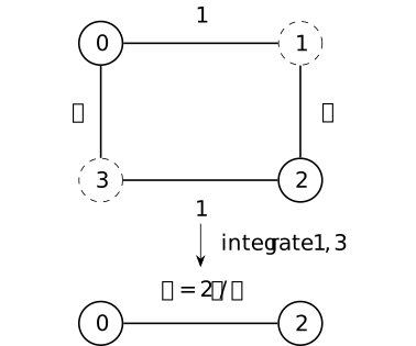
Solid circles are retained; dashed circles are integrated out. Orientations are suppressed because the quadratic energy is orientation independent. The bottom edge represents the induced coupling \(\beta \); its precision also has the diagonal term computed below.
The vectors \((1,1)^T/\sqrt 2\) and \((1,-1)^T/\sqrt 2\) diagonalize \(S\). Their eigenvalues are \[\begin {aligned} \sigma _+&=\alpha -\beta =\frac {s^2-(1+t)^2}{s}\\ &=\frac {a(a+2+2t)}{s},\\ \sigma _-&=\alpha +\beta =\frac {s^2-(1-t)^2}{s}\\ &=\frac {(a+2)(a+2t)}{s}. \end {aligned}\] Both are positive. The factorizations follow from \(s=1+t+a\); they also check positivity without appealing again to the general theorem. Put \[\mathcal D=a(a+2)(a+2t)(a+2+2t).\] Then \[\begin {aligned} \det C&=s^2,\qquad \det S=\mathcal D/s^2,\\ \det Q&=\det C\det S=\mathcal D,\\ c_C&=\frac {2\pi }{s},\qquad Z_S=\frac {2\pi s}{\sqrt {\mathcal D}},\\ Z_Q&=c_CZ_S=\frac {(2\pi )^2}{\sqrt {\mathcal D}}. \end {aligned}\] This reproduces the four-mode determinant and partition function. The effective action is \[\mathcal A_{\mathrm {eff}}(x)=\tfrac 12x^TSx+\log \frac {s}{2\pi }.\] Its constant records the integrated block.
A retained observable checks more than normalization. For \(F(x)=x_0x_2\), polynomial integrability and the marginal identity give \[\begin {aligned} \langle \phi _0\phi _2\rangle _Q &=\langle x_0x_2\rangle _S =(S^{-1})_{02}\\ &=\frac {\beta }{\alpha ^2-\beta ^2} =\frac {2ts}{\mathcal D}. \end {aligned}\] The indices \(0,2\) here name retained vertices. Inverting the displayed two-by-two matrix gives its off-diagonal entry \(\frac {\beta }{\det S}\), which proves the last equalities. Independently, the four-cycle spectral table gives \[\begin {aligned} 4\langle \phi _0\phi _2\rangle _Q &=\frac 1a-\frac 1{a+2}\\ &\quad -\frac 1{a+2t}+\frac 1{a+2+2t}\\ &=\frac {8ts}{\mathcal D}. \end {aligned}\] For the last equality, pair the first two terms and the last two: their difference has numerator \(2((a+2t)(a+2+2t)-a(a+2))=8ts\) over \(\mathcal D\). At \(t=m=1\), one obtains \[\begin {aligned} S&=\begin {pmatrix}7/3&-2/3\\-2/3&7/3\end {pmatrix},\\ S^{-1}&=\frac 1{15}\begin {pmatrix}7&2\\2&7\end {pmatrix},\\ \langle \phi _0\phi _2\rangle _Q&=\frac {2}{15},\\ c_C&=\frac {2\pi }{3},\quad Z_S=\frac {2\pi }{\sqrt 5},\quad Z_Q=\frac {4\pi ^2}{3\sqrt 5}. \end {aligned}\] Fixing the eliminated fields to zero instead gives precision \(A=3I_2\), covariance \(I_2/3\) and zero off-diagonal covariance. At \(t=2,m=1\), the same formulas give \[\begin {aligned} S&=\begin {pmatrix}11/4&-1\\-1&11/4\end {pmatrix},\\ \det S&=105/16,\\ S^{-1}&=\frac 1{105}\begin {pmatrix}44&16\\16&44\end {pmatrix}. \end {aligned}\] These are the parameters used in the symmetry comparison.
In the orthonormal sector coordinates \(x_\pm =(x_0\pm x_2)/\sqrt 2\) and \(y_\pm =(y_1\pm y_3)/\sqrt 2\), the couplings are \(-(1+t)\) and \(-(1-t)\). Their two eliminated pivots are both \(s\); each contributes \(\sqrt {2\pi/s}\), whose product is \(2\pi/s\). The factors \(1/\sqrt 2\) make these changes orthogonal, so there is no extra volume factor. The retained variance is \(\frac 12(\sigma _+^{-1}+\sigma _-^{-1})\), and the opposite covariance is \(\frac 12(\sigma _+^{-1}-\sigma _-^{-1})\). This agrees with the sector calculation.
There was no edge between vertices \(0\) and \(2\) in the supplied cycle. Elimination induces one in the effective quadratic form: \[S=\beta \begin {pmatrix}1&-1\\-1&1\end {pmatrix} +\sigma _+I_2.\] Thus \(\beta \) is an effective edge weight and \(\sigma _+\) an effective mass coefficient. This is a finite instance of fill-in: eliminating a single vertex joined to retained vertices with weights \(w_i\) and diagonal precision \(c>0\) subtracts \(ww^T/c\), creating off-diagonal entries \(-w_iw_j/c\) where no retained edge existed. The formula is the same Schur complement with \(H=-w\) and \(C=(c)\). Locality in the original graph need not survive elimination.
The half-turn preserves both sets \(R,U\) and swaps the two coordinates within each. For the swap matrix \(J\), the displayed \(S\) satisfies \(JSJ=S\); the induced two-site form retains this symmetry. The density and orthogonal-volume invariance then show that the retained law is invariant as well.
At \(m=0\), \(C=(1+t)I_2\) remains positive. Square completion and integration over the eliminated block still give \[S=\frac {2t}{1+t}\begin {pmatrix}1&-1\\-1&1\end {pmatrix}, \qquad c_C=\frac {2\pi }{1+t}.\] The retained constant mode has zero energy, so its full integral diverges by the kernel-box argument. The finite fiber factor cannot be divided by a finite retained partition function.
The global mean-zero law instead uses the space \(H=\{\phi :\sum _v\phi _v=0\}\) with its own induced volume. Its constraint \(x_0+x_2+y_1+y_3=0\) couples the two parts; \(H\) is neither their unrestricted product nor the product of their separate mean-zero lines. At \(t=1\), write a field in the three positive orthonormal modes as \(\phi =z_1u_1+z_2u_2+z_3u_3\). The coordinates are independent centered Gaussians of precisions \(2,2,4\). Put \[r=\frac {z_1+z_2}{\sqrt 2},\qquad v=\frac {z_1-z_2}{\sqrt 2}.\] This orthogonal change preserves \(z_1^2+z_2^2=r^2+v^2\) and two-dimensional volume. Thus \(r,v,z_3\) still have independent centered Gaussian laws of precisions \(2,2,4\). The retained unit coordinates satisfy \[\begin {aligned} x_-&=(\phi _0-\phi _2)/\sqrt 2=r,\\ x_+&=(\phi _0+\phi _2)/\sqrt 2=z_3/\sqrt 2. \end {aligned}\] Integrating the normalized \(v\) factor and changing variable \(z_3=\sqrt 2x_+\) give independent retained Gaussian densities of precisions \(2\) and \(8\). This density calculation identifies the law, not merely its covariance. Returning orthogonally to \((x_0,x_2)\) gives \[\begin {aligned} \operatorname {Cov}(x)&=\frac 1{16} \begin {pmatrix}5&-3\\-3&5\end {pmatrix},\\ Q_{H\to R}&=\begin {pmatrix}5&3\\3&5\end {pmatrix}. \end {aligned}\] These matrices multiply to the identity. The projected normalizer for this precision is \(\frac {2\pi }{\sqrt {16}}=\frac \pi 2\).
In contrast, directly setting \(m=0,t=1\) in the Schur formula gives the singular precision \(\begin {pmatrix}1&-1\\-1&1\end {pmatrix}\). Separately constraining that retained model to \(x_0+x_2=0\) leaves unit direction \((1,-1)/\sqrt 2\) with precision \(2\), normalizer \(\sqrt \pi \) and ambient covariance \(\frac 14\begin {pmatrix}1&-1\\-1&1\end {pmatrix}\). These are three distinct specified measures. The pinned affine law is another constraint with its own induced volume; fixing a vertex is not the marginal operation above.
The arithmetic pivot boundary is separate from the positive-real case. At \(m^2=1,t=-2\), \(s=t+2=0\), whereas \(\det Q=1\cdot 3\cdot (-3)\cdot (-1)=9\). Thus the full map can be invertible while this eliminated pivot is not. At \(t=-1\), the pivot exists but the later ratio denominator \(t+1\) vanishes. Neither value satisfies the positive-weight hypotheses used for the Gaussian laws here.
Proposition 6. Formal interaction under Gaussian elimination [fdip-0046]AGENTDRAFTED
- October 30, 2026
Proposition 6. Formal interaction under Gaussian elimination [fdip-0046]AGENTDRAFTED
- October 30, 2026
Eliminating a field with a quartic interaction generally creates quadratic and sextic terms. The coefficients through second order can be found by conditional Gaussian moments, while preserving a supplied symmetry and composition of eliminations.
Use the finite orthogonal sum \(E=X\mathbin \perp Y\), positive precision \(Q\), components \(A,B,C\), Schur precision \(S\) and scalar \(c_C\) of Gaussian elimination. Let \(T:E^4\to \mathbb R\) be a symmetric four-linear form and put \[V(u)=\frac {T(u,u,u,u)}{4!}.\] Write \(\mathcal P(X)\) for the polynomial function algebra. For \(x\in X\), let \(\eta \) have centered Gaussian law with covariance \(C^{-1}\) on \(Y\), and set \[v_x=(x,-C^{-1}B^\dagger x+\eta ).\] This is the conditional law of the eliminated field given the retained value. It is the conditional kernel with its two named summands exchanged; its covariance is \(C^{-1}\), whereas that proposition's retained-given-eliminated kernel has covariance \(A^{-1}\).
For a formal variable \(\lambda \), use ordinary power-series coefficients in \(\lambda \) and define the fiber effective interaction by \[\begin {aligned} F_\lambda (x)&=-\log \mathbb E_\eta e^{-\lambda V(v_x)},\\ \mathbb E_\eta e^{-\lambda V(v_x)} &=\sum _{n\geq 0}\frac {(-\lambda )^n}{n!} \mathbb E_\eta V(v_x)^n. \end {aligned}\] These are formal series in \(\lambda \) with coefficients in \(\mathcal P(X)\); the logarithm is the formal logarithm of a series with constant coefficient one. Every coefficient is finite by polynomial integrability. The notation \(O(\lambda ^3)\) means a series divisible by \(\lambda ^3\), not an analytic error estimate. With \[\begin {aligned} a(x)&=\mathbb E[V\mid x],\\ b(x)&=\mathbb E[V^2\mid x]-a(x)^2, \end {aligned}\] the first two coefficients are \[F_\lambda =\lambda a-\frac {\lambda ^2}{2}b+O(\lambda ^3).\] The degree-zero terms are retained: coefficientwise integration gives \[\begin {aligned} &\int _Y e^{-\frac 12\langle (x,y),Q(x,y)\rangle } e^{-\lambda V(x,y)}\,dy\\ &\qquad =c_Ce^{-\frac 12\langle x,Sx\rangle }e^{-F_\lambda (x)}. \end {aligned}\] Here \(dy\) is the specified Euclidean volume. This fiber logarithm integrates eliminated variables; it does not take the Legendre transform of a source-generating function used for a one-particle irreducible (1PI) effective action in [etingof2024mathematical, v2, Proposition 3.23, p. 50].
For a specified orthogonal flag \(E=X\mathbin \perp Y\mathbin \perp Z\), first eliminate \(Z\) and then \(Y\). All conditional expectations below use the original Gaussian law, with the \(Y\)-given-\(X\) kernel obtained after eliminating \(Z\). Put \[\begin {aligned} a_1(x,y)&=\mathbb E[V\mid x,y],\\ b_1(x,y)&=\mathbb E[V^2\mid x,y]-a_1(x,y)^2. \end {aligned}\] Both stages together give \[\begin {aligned} F_\lambda (x) ={}&\lambda \mathbb E[a_1\mid x]\\ &-\frac {\lambda ^2}{2}\bigl ( \mathbb E[b_1\mid x]+\operatorname {Var}(a_1\mid x)\bigr )\\ &+O(\lambda ^3), \end {aligned}\] which agrees with direct elimination of \(Y\oplus Z\). The first coefficient has degrees among \(4,2,0\); the second has degrees among \(6,4,2,0\). Particular components may vanish.
Proof.
- October 30, 2026
Proof.
- October 30, 2026
Expand the expectation as \(1-\lambda a+\lambda ^2\mathbb E[V^2\mid x]/2+O(\lambda ^3)\). The identity \(\log (1+u)=u-u^2/2+O(u^3)\) gives the displayed coefficient \(-b/2\). Square completion in Theorem 1 identifies the normalized conditional Gaussian and the raw scalar \(c_C\); applying it to each polynomial coefficient proves the fiber identity. No convergence or interchange of an infinite series and an integral is needed.
The first-stage interaction is \(F_1=\lambda a_1-\lambda ^2b_1/2+O(\lambda ^3)\). Hence \[e^{-F_1}=1-\lambda a_1+ \frac {\lambda ^2}{2}(a_1^2+b_1)+O(\lambda ^3).\] Take the \(Y\)-given-\(X\) expectation and the negative logarithm. This yields the stated two-stage formula. Polynomial integrability permits signed Fubini for every coefficient, so the tower identities for these Gaussian kernels give \[\begin {aligned} &\mathbb E[a_1\mid x]=\mathbb E[V\mid x],\\ &\mathbb E[b_1\mid x]+\operatorname {Var}(a_1\mid x)\\ &\qquad =\mathbb E[V^2\mid x]-\mathbb E[V\mid x]^2. \end {aligned}\] These identities also follow directly by expanding \(b_1\) and cancelling \(\mathbb E[a_1^2\mid x]\). They prove composition through the stated order without discarding any generated term.
The mean of \(v_x\) is linear in \(x\), and its centered noise is independent of \(x\). Expanding the four-linear tensor and pairing centered Gaussian factors by Wick's theorem leaves degrees \(4,2,0\) in \(a\). In \(\mathbb E[V^2\mid x]-\mathbb E[V\mid x]^2\), pairings with no contraction between the two copies of \(V\) cancel. Every remaining pairing uses at least two noise factors. The 8 original factors therefore leave at most 6 mean factors. An even number of noise factors is paired, giving only degrees \(6,4,2,0\). The homogeneous components are symmetric tensors on \(X\) by polarization; they need not be diagonal in a chosen coordinate basis.
Suppose a second such model is related by a linear isometric isomorphism \(L=L_X\oplus L_Y:E\to E'\) satisfying \(Q'L=LQ\) and \(V'\circ L=V\). Then \[F'_\lambda (L_Xx)=F_\lambda (x)\pmod {\lambda ^3}.\] Indeed the component identities give \(C'L_Y=L_YC\) and \((B')^\dagger L_X=L_YB^\dagger \). Thus \(L_Y\) transports the conditional mean and covariance, hence its Gaussian law and both moments \(a,b\). For two-stage elimination also require preservation of the supplied flag. In particular, a supplied finite group of these isometries preserves each induced coefficient. The result transports a given action; it does not select that action.
Wick contractions are [etingof2024mathematical, v2, Theorem 3.1 and Example 3.2, p. 29]. The perturbation convention in [etingof2024mathematical, v2, Section 3.3, p. 33] is \(B(u,u)/2-\sum _i g_iB_i(u,\ldots ,u)/i!\); here \(g_4=-\lambda \) and \(B_4=T\), at \(\hbar =1\). The conditional formulas and composition above are direct deductions using these contractions and the specified Gaussian kernels. The three-coordinate example exhibits every indicated degree.
Example 7. A quartic interaction and its retained four-point function [fdip-0047]AGENTDRAFTED
- October 30, 2026
Example 7. A quartic interaction and its retained four-point function [fdip-0047]AGENTDRAFTED
- October 30, 2026
On the real realization of \(\mathbb Q^3\), use coordinates \(x,y,z\), counting pairing \(g_0=I\) and the coordinate flag retaining \((x,y)\) and then \(x\). Fix the action \(q/2+\lambda V\), where \[\begin {aligned} q&=x^2+(y-x)^2+(z-y)^2,\\ V&=\frac {x^4+y^4+z^4}{4!},\\ Q&=\begin {pmatrix}2&-1&0\\-1&2&-1\\0&-1&1\end {pmatrix},\\ Q^{-1}&=\begin {pmatrix}1&1&1\\1&2&2\\1&2&3\end {pmatrix}. \end {aligned}\] The quadratic form is positive: the map \((x,y,z)\mapsto (x,y-x,z-y)\) is invertible. The fourth tensor of \(V\) has diagonal components one and all other components zero, with the displayed \(1/4!\) convention. Simultaneous sign reversal supplies an action of \(C_2\) preserving the pairing, action and flag.
For the fiber interaction after eliminating \(y,z\), the retained precision is \(S=1\), the scalar is \(c_C=2\pi \), and \[\begin {aligned} F_\lambda (x) ={}&\lambda \left (\frac {x^4}{8}+\frac {3x^2}{4}+\frac 58\right )\\ &-\lambda ^2\left (\frac {5x^6}{72}+\frac {53x^4}{48}\right .\\ &\hspace {38pt}\left .+\frac {97x^2}{24}+\frac {41}{24}\right ) +O(\lambda ^3). \end {aligned}\] In particular, a pure quartic interaction is not preserved by elimination. Adding a quadratic term and a constant still does not close this family: the second-order sextic coefficient is nonzero.
Proof.
- October 30, 2026
Proof.
- October 30, 2026
Under the Gaussian law conditional on \(x\), write \(y=x+\eta \) and \(z=x+\eta +\xi \), where \(\eta ,\xi \) are independent standard real Gaussians. This follows directly from \(q=x^2+\eta ^2+\xi ^2\) and the triangular change of variables of determinant one. Thus \[C^{-1}=\begin {pmatrix}1&1\\1&2\end {pmatrix}, \qquad S=1,\qquad c_C=2\pi .\] With \(a=\mathbb E[V\mid x]\) and \(b=\operatorname {Var}(V\mid x)\), use \(\mathbb E\eta ^{2k}=(2k-1)!!\), with \((-1)!!=1\), and zero odd moments. The first moments are \[\begin {aligned} \mathbb E[y^4\mid x]&=x^4+6x^2+3,\\ \mathbb E[z^4\mid x]&=x^4+12x^2+12. \end {aligned}\] For the second coefficient, the same pairings give \[\begin {aligned} \operatorname {Var}(y^4\mid x) &=16x^6+168x^4\\ &\quad +384x^2+96,\\ \operatorname {Var}(z^4\mid x) &=32x^6+672x^4\\ &\quad +3072x^2+1536,\\ \operatorname {Cov}(y^4,z^4\mid x) &=16x^6+216x^4\\ &\quad +600x^2+168. \end {aligned}\] For instance these mixed moments use \(\mathbb E\eta ^2=1\), \(\mathbb E(\eta +\xi )^2=2\) and \(\mathbb E[\eta (\eta +\xi )]=1\). The term \(x^4\) is constant at fixed \(x\), so \[\begin {aligned} a&=\frac {x^4}{8}+\frac {3x^2}{4}+\frac 58,\\ b&=\frac {5x^6}{36}+\frac {53x^4}{24} +\frac {97x^2}{12}+\frac {41}{12}. \end {aligned}\] Substitute these into \(F_\lambda =\lambda a-\lambda ^2b/2+O(\lambda ^3)\).
The same coefficients arise in two stages. First eliminate \(z=y+\xi \) with \(x,y\) fixed. The moments above, with \(x\) replaced by \(y\), give \[\begin {aligned} a_1(x,y)&=\frac {x^4+2y^4+6y^2+3}{24},\\ b_1(x,y)&=\frac {y^6}{36}+\frac {7y^4}{24} +\frac {2y^2}{3}+\frac 16. \end {aligned}\] Here \(a_1=\mathbb E[V\mid x,y]\) and \(b_1=\operatorname {Var}(V\mid x,y)\); the terms \(x^4,y^4\) are constant at this stage. Next take \(y=x+\eta \). The even moments \(1,3,15,105\) of orders \(2,4,6,8\) give \[\begin {aligned} \mathbb E[a_1\mid x]&=\frac {x^4}{8}+\frac {3x^2}{4}+\frac 58=a,\\ \mathbb E[b_1\mid x]&=\frac {x^6}{36}+\frac {17x^4}{24} +\frac {11x^2}{3}+\frac {17}{8},\\ \operatorname {Var}(a_1\mid x)&=\frac {x^6}{9}+\frac {3x^4}{2} +\frac {53x^2}{12}+\frac {31}{24}. \end {aligned}\] The last two lines sum to \(b\). Thus the two-stage identity reproduces both direct coefficients, including their constants.
A source on a retained space \(X\) is a linear functional \(j\in X^*\), coupled by multiplying the weight by \(e^{j(x)}\). Under a retained linear isomorphism \(L_X:X\to X'\), a source \(j'\in (X')^*\) pulls back to \(j'\circ L_X\), since \(e^{j'(L_Xx)}=e^{(j'\circ L_X)(x)}\). In this example \(X=\mathbb R\) and \(j(x)=Jx\), with \(J\) treated as a formal scalar variable. Let \(\mu _Q\) be the normalized Gaussian law. Define \[\begin {aligned} W(J,\lambda ) ={}&\log \mathbb E_{\mu _Q}e^{Jx-\lambda V}\\ &-\log \mathbb E_{\mu _Q}e^{-\lambda V}. \end {aligned}\] Each coefficient in the two formal variables \(J,\lambda \) is a finite Gaussian moment. Thus \(W(0,\lambda )=0\). Coefficients use ordinary powers of \(\lambda \); 4 source derivatives multiply the coefficient of \(J^4\) by \(4!\). The connected four-point function in this scalar example is \[\begin {aligned} G_c^{(4)}(\lambda ) &=\left .\frac {\partial ^4W}{\partial J^4}\right |_{J=0}\\ &=-3\lambda +101\lambda ^2+O(\lambda ^3). \end {aligned}\]
Proof.
- October 30, 2026
Proof.
- October 30, 2026
Write \[\mathbb E_\lambda [P]= \frac {\mathbb E_{\mu _Q}[P e^{-\lambda V}]} {\mathbb E_{\mu _Q}e^{-\lambda V}}\] as a formal ratio. After eliminating \(y,z\), both numerator and denominator are expectations for \(x\sim N(0,1)\) with weight \[\begin {aligned} e^{-F_\lambda (x)}={}&1-\lambda a(x)\\ &+\frac {\lambda ^2}{2}(a(x)^2+b(x))\\ &+O(\lambda ^3). \end {aligned}\] The scalar \(c_C\) cancels from this ratio, but the constant terms in \(a,b\) are included before the division. Gaussian moments give \[\begin {aligned} \mathbb E[e^{-F_\lambda }]&= 1-\frac 74\lambda +\frac {1351}{96}\lambda ^2+O(\lambda ^3),\\ \mathbb E[x^2e^{-F_\lambda }]&= 1-\frac {19}{4}\lambda +\frac {1981}{32}\lambda ^2+O(\lambda ^3),\\ \mathbb E[x^4e^{-F_\lambda }]&= 3-\frac {105}{4}\lambda +\frac {14799}{32}\lambda ^2\\ &\qquad +O(\lambda ^3). \end {aligned}\] Dividing yields \[\begin {aligned} \mathbb E_\lambda [x^2]&= 1-3\lambda +\frac {511}{12}\lambda ^2+O(\lambda ^3),\\ \mathbb E_\lambda [x^4]&= 3-21\lambda +\frac {767}{2}\lambda ^2+O(\lambda ^3). \end {aligned}\] Sign reversal makes the odd moments zero and \(W(-J,\lambda )=W(J,\lambda )\). Expanding the logarithm in \(J\) therefore gives \[G_c^{(4)}=\mathbb E_\lambda [x^4] -3\bigl (\mathbb E_\lambda [x^2]\bigr )^2,\] which is the asserted coefficient.
These are formal expansions. For real \(\lambda \geq 0\), the original interaction is nonnegative, so its exact partition integral is positive and bounded by the Gaussian normalizer. Polynomial moments remain finite. A real source also gives a finite integral, since the linear tilt of a positive Gaussian is integrable. None of this asserts convergence of the formal series at zero. For every fixed \(\lambda >0\), exponentiating only the displayed second-order \(F_\lambda \) instead gives a nonintegrable retained weight: its leading term is \(-5\lambda ^2x^6/72\), so \(e^{-x^2/2-F_\lambda ^{(2)}(x)}\) grows at infinity. Here \(F_\lambda ^{(2)}\) denotes the displayed polynomial through \(\lambda ^2\).
The Gaussian moment rule is [etingof2024mathematical, v2, Theorem 3.1, p. 29]. The connected-logarithm interpretation is [etingof2024mathematical, v2, Theorem 3.11, p. 38], with \(g_4=-\lambda \) and the zero-source logarithm subtracted. The rational coefficients above are the explicit calculation for this supplied model. Stationary elimination retains its sextic term but omits the fluctuation-generated lower degrees.
Remark 8. Stationary elimination and the tree contribution [fdip-0048]AGENTDRAFTED
- October 30, 2026
Remark 8. Stationary elimination and the tree contribution [fdip-0048]AGENTDRAFTED
- October 30, 2026
For the three-coordinate quartic action, formal power-series stationarity around the Gaussian stationary point and integration of the eliminated fluctuations agree on some coefficients but not all. Write \(u=(y,z)\), \(u_0=(x,x)\) and \[H=C^{-1}=\begin {pmatrix}1&1\\1&2\end {pmatrix}.\] At fixed \(x\), the action is \[\begin {aligned} \mathcal A(x,u)={}&\frac {x^2}{2} +\frac 12(u-u_0)^TC(u-u_0)\\ &+\lambda V(x,u). \end {aligned}\] There is a unique formal stationary solution \(u_*(x,\lambda )=u_0+O(\lambda )\). Its stationary value is \[\begin {aligned} \mathcal A_{\mathrm {cl}}(x,\lambda ) &=\mathcal A(x,u_*(x,\lambda ))\\ &=\frac {x^2}{2}+\frac {\lambda x^4}{8} -\frac {5\lambda ^2x^6}{72}+O(\lambda ^3). \end {aligned}\] For real \(\lambda \geq 0\), the action is coercive and strictly convex in \(u\): the quadratic Hessian \(C\) is positive definite and the quartic summands are convex. It therefore has a unique minimizer. The calculation below uses only formal power-series stationarity around \(u_0\) at \(\lambda =0\).
Proof.
- October 30, 2026
Proof.
- October 30, 2026
The equation is \(C(u-u_0)+\lambda \nabla _uV(x,u)=0\). Since \(C\) is invertible, comparison of successive powers of \(\lambda \) uniquely determines the formal coefficients. Put \[r=\nabla _uV(x,u_0)=\frac {x^3}{6}\binom {1}{1}.\] The first coefficient gives \(u_*=u_0-\lambda Hr+O(\lambda ^2)\). Substitution in the action yields \[\mathcal A_{\mathrm {cl}}= \frac {x^2}{2}+\lambda V(x,u_0) -\frac {\lambda ^2}{2}r^THr+O(\lambda ^3).\] Now \(V(x,u_0)=x^4/8\) and \(r^THr=5x^6/36\). This proves the stationary coefficient without replacing a Gaussian integral by a minimum.
To distinguish fluctuation terms, take \(\hbar >0\), let \(\eta _\hbar \) be centered Gaussian with covariance \(\hbar H\), and use the normalized fiber expression \[\begin {aligned} &F_{\lambda ,\hbar }(x)\\ &\quad =-\hbar \log \mathbb E\exp \left ( -\frac {\lambda }{\hbar }V(x,u_0+\eta _\hbar )\right ). \end {aligned}\] Expand formally in \(\lambda \); through the second order its coefficients are polynomials in \(\hbar \): \[\begin {aligned} F_{\lambda ,\hbar }(x) ={}&\lambda \left (\frac {x^4}{8}+\frac {3\hbar x^2}{4} +\frac {5\hbar ^2}{8}\right )\\ &-\lambda ^2\left (\frac {5x^6}{72} +\frac {53\hbar x^4}{48}\right .\\ &\hspace {38pt}\left .+\frac {97\hbar ^2x^2}{24} +\frac {41\hbar ^3}{24}\right )\\ &+O(\lambda ^3). \end {aligned}\] Indeed each Gaussian pairing contributes one \(\hbar \); the first coefficient is \(\mathbb E V\) and the second is \(-\operatorname {Var}(V)/(2\hbar )\). Applying this scaling to the explicit moment calculation proves the formula.
Consequently, through order \(\lambda ^2\), the coefficient of \(\hbar ^0\) in this fiber interaction is \[\begin {aligned} [\hbar ^0]F_{\lambda ,\hbar }(x) &=\frac {\lambda x^4}{8}-\frac {5\lambda ^2x^6}{72} +O(\lambda ^3)\\ &=\mathcal A_{\mathrm {cl}}(x,\lambda )-\frac {x^2}{2} +O(\lambda ^3). \end {aligned}\] The retained Gaussian action \(x^2/2\) must be added to recover the full stationary value. At \(\lambda =0\) the normalized fiber interaction is zero, whereas that stationary value is \(x^2/2\).
This is the tree contribution in the loop grading of [etingof2024mathematical, v2, Section 3.6 and Theorem 3.12, pp. 38-39]. We adapt Etingof's rescaled convention to the displayed weight \(\exp (-\lambda V/\hbar )\) with covariance \(\hbar H\): a Gaussian contraction contributes \(\hbar \) and an interaction vertex contributes \(\hbar ^{-1}\). The logarithm selects connected graphs; after multiplication by \(-\hbar \), a connected graph with \(e\) contracted edges and \(v\) interaction vertices has power \(\hbar ^{e-v+1}\). Its number of independent cycles is \(e-v+1\); zero cycles means a tree. Thus connected contractions need not be trees. In the displayed second-order coefficient, only the sextic term is at tree order; its quartic, quadratic and constant companions have positive powers of \(\hbar \). The source's stationary-action convention is applied to the shifted fiber action, whose unperturbed minimum is zero, which explains the subtraction of \(x^2/2\).
The retained law still refers to chosen field coordinates and a chosen split. Which changes merely relabel and transport this model, and which change its predictions?