Eliminating a chosen summand [fdip-0020]
✍️sourceAGENTDRAFTED
- October 23, 2026
Eliminating a chosen summand [fdip-0020]
✍️sourceAGENTDRAFTED
- October 23, 2026
When some field values can be solved for, which equation remains on the others? A chosen partition gives one splitting of a field module. More generally, a specified split module and an invertible eliminated component determine a retained linear map. Triangular factorization explains its inverse and kernel before any pairing or probability law is chosen.
Perfect symmetric pairings turn this factorization into a congruence when the splitting is orthogonal. Positive real inner products then give the Schur positivity criterion, and cycle elimination makes the retained inverse comparison explicit. The later Gaussian elimination adds the measure and normalization needed to interpret a retained marginal.
Definition 1. Components of a split endomorphism [fdip-001T]AGENTDRAFTED
- October 23, 2026
Definition 1. Components of a split endomorphism [fdip-001T]AGENTDRAFTED
- October 23, 2026
To eliminate part of a field, first choose which part is retained. Let \(R\) be a commutative unital ring and \(M,X,Y\) unital \(R\)-modules. A chosen binary splitting of \(M\) consists of ordinary \(R\)-linear maps \[\iota _X:X\to M,\quad \iota _Y:Y\to M,\qquad \pi _X:M\to X,\quad \pi _Y:M\to Y\] satisfying all 5 identities \[\begin {aligned} \pi _X\iota _X&=I_X,&\pi _Y\iota _Y&=I_Y,\\ \pi _X\iota _Y&=0,&\pi _Y\iota _X&=0,\\ \iota _X\pi _X+\iota _Y\pi _Y&=I_M. \end {aligned}\] Products apply the right factor first, as in composition and field multiplication. The maps \((x,y)\mapsto \iota _Xx+\iota _Yy\) and \(z\mapsto (\pi _Xz,\pi _Yz)\) are inverse linear maps by these identities. We consequently write \(M=X\oplus Y\) and \(z=(x,y)\) relative to this chosen identification.
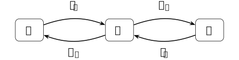
Each summand is included in \(M\) and recovered by its projection. The composite \(\pi _X\iota _X\) is \(I_X\), whereas \(\iota _X\pi _X\) is an endomorphism of \(M\). In the partition realization, these are restriction and extension by zero; the latter composite is the support projection.
For an endomorphism \(Q:M\to M\), its components for the chosen splitting are \[\begin {aligned} A&=\pi _XQ\iota _X:X\to X,&B&=\pi _XQ\iota _Y:Y\to X,\\ E&=\pi _YQ\iota _X:X\to Y,&C&=\pi _YQ\iota _Y:Y\to Y. \end {aligned}\] Inserting \(I_M=\iota _X\pi _X+\iota _Y\pi _Y\) gives \[Q(x,y)=(Ax+By,Ex+Cy).\] If the eliminated component \(C\) is an isomorphism, define the split Schur map, relative to this splitting and pivot, by \[S=A-BC^{-1}E:X\longrightarrow X.\] Changing the splitting or the pivot changes the construction.
The module convention is
[stacks2017stacks, Section 10.10], Tag 0581.
Mathlib's CategoryTheory.Biprod.ofComponents gives
components in a preadditive category with binary biproducts.
Its arguments index source then target; after ordering summands
\((Y,X)\), the arguments corresponding to \(Q\) are \((C,B,E,A)\).
[boyd2004convex, Appendix A.5.5, pp. 650-651] treats the real Schur complement. The source eliminates its first block: exchanging its variables to \((y,x)\) makes its block order \((C,E,B,A)\) and its residual \(A-BC^{-1}E\). The chosen-splitting definition above uses only linear maps; it does not assume a basis, pairing or positivity.
The ring elimination example computes the components and Schur map for a concrete chosen splitting.
Theorem 2. Triangular factorization of a split map [fdip-001U]AGENTDRAFTED
- October 23, 2026
Theorem 2. Triangular factorization of a split map [fdip-001U]AGENTDRAFTED
- October 23, 2026
Let \(R\) be a commutative unital ring and \(M=X\oplus Y\) a chosen binary splitting of unital \(R\)-modules. Let \(Q(x,y)=(Ax+By,Ex+Cy)\) have the typed components of this splitting, and assume \(C:Y\to Y\) is an isomorphism. Set \[K=C^{-1}E:X\to Y,\qquad S=A-BC^{-1}E:X\to X.\] Define three endomorphisms of \(M\) by \[\begin {aligned} U(x,y)&=(x+BC^{-1}y,y),\\ D(x,y)&=(Sx,Cy),\\ V(x,y)&=(x,y+Kx). \end {aligned}\] Then \(U,V\) are isomorphisms and, with right-factor-first composition, \[Q=UDV.\]
Proof.
- October 23, 2026
Proof.
- October 23, 2026
The displayed maps are linear since every component is linear. Direct substitution on both sides verifies the inverses \[U^{-1}(x,y)=(x-BC^{-1}y,y),\qquad V^{-1}(x,y)=(x,y-Kx).\] These inverses require no inverse of \(S\). Applying the three factors in order gives \[\begin {aligned} DV(x,y)&=(Sx,Ex+Cy),\\ UDV(x,y)&=(Sx+BC^{-1}(Ex+Cy),Ex+Cy)\\ &=(Ax+By,Ex+Cy)=Q(x,y), \end {aligned}\] where \(S+BC^{-1}E=A\) and \(C^{-1}C=I_Y\) give the last equality.
[boyd2004convex, Appendix C.4.1, pp. 672-673] gives real block-system elimination. The proof above extends it directly to modules. The source uses first-pivot order; swapping to the eliminated summand gives the convention here. No finite rank, projectivity or determinant is used.
Mathlib's CategoryTheory.Biprod.gaussian'
supports elimination in a preadditive category with binary biproducts
and an invertible first component. In the order \((Y,X)\), use
\((C,B,E,A)\) as its component arguments. Its notation \(f\gg g\)
applies \(f\) first, so its residual is \(A-BC^{-1}E\).
For finite coordinate index types,
Matrix.fromBlocks_eq_of_invertible₂₂ gives the corresponding
matrix factorization over a commutative ring; its 4 arguments become
\((A,B,E,C)\). These support the factorization, while the subsequent
inverse and kernel
statements have their own proofs.
Theorem 3. Inverse components and retained compression [fdip-001V]AGENTDRAFTED
- October 23, 2026
Theorem 3. Inverse components and retained compression [fdip-001V]AGENTDRAFTED
- October 23, 2026
Over a commutative unital ring \(R\), let \(M=X\oplus Y\) be a chosen splitting, with ordinary linear endomorphism \(Q(x,y)=(Ax+By,Ex+Cy)\). Assume that the eliminated component \(C\) is an isomorphism, and put \(S=A-BC^{-1}E\). Then \(Q\) is an isomorphism if and only if \(S\) is an isomorphism. When these conditions hold, all 4 components of the inverse are \[\begin {aligned} \pi _XQ^{-1}\iota _X&=S^{-1}:X\to X,\\ \pi _XQ^{-1}\iota _Y&=-S^{-1}BC^{-1}:Y\to X,\\ \pi _YQ^{-1}\iota _X&=-C^{-1}ES^{-1}:X\to Y,\\ \pi _YQ^{-1}\iota _Y&=C^{-1}+C^{-1}ES^{-1}BC^{-1}:Y\to Y. \end {aligned}\] In particular, the retained compression of \(Q^{-1}\) is \(S^{-1}\); it is not in general \(A^{-1}\).
Proof.
- October 23, 2026
Proof.
- October 23, 2026
Use \(Q=UDV\) and the explicit inverses of \(U,V\) from triangular factorization, where \(D(x,y)=(Sx,Cy)\). If \(S\) is invertible, then \(D^{-1}(u,v)=(S^{-1}u,C^{-1}v)\). Thus \(Q^{-1}=V^{-1}D^{-1}U^{-1}\) is a two-sided inverse.
Conversely, suppose \(Q\) is invertible. Then \(D=U^{-1}QV^{-1}\) is invertible; write \(J=D^{-1}\) and set \(J_X=\pi _XJ\iota _X:X\to X\). The identities \(\pi _XD=S\pi _X\) and \(D\iota _X=\iota _XS\) imply \[\begin {aligned} SJ_X&=\pi _XDJ\iota _X=\pi _X\iota _X=I_X,\\ J_XS&=\pi _XJD\iota _X=\pi _X\iota _X=I_X. \end {aligned}\] Hence \(J_X\) is a two-sided inverse of \(S\). This implication still uses the assumed invertibility of \(C\).
Applying the three inverse factors to \((u,v)\) gives \[\begin {aligned} x&=S^{-1}u-S^{-1}BC^{-1}v,\\ y&=-C^{-1}ES^{-1}u +(C^{-1}+C^{-1}ES^{-1}BC^{-1})v. \end {aligned}\] Setting one input component to zero and projecting the other gives the 4 stated map identities.
The real symmetric inverse formula is
[boyd2004convex, Appendix A.5.5, p. 650]; its first-pivot
convention is exchanged here. The direct proof uses arbitrary unital
\(R\)-modules and needs no pairing or symmetry.
Mathlib's CategoryTheory.Biprod.isoElim' constructs
the residual isomorphism when both the first component and the whole
biproduct map are isomorphisms. With summands \((Y,X)\) and component
arguments \((C,B,E,A)\), it supports the whole-to-residual direction;
it does not by itself assert the 4 inverse formulas above.
For a self-adjoint precision with a chosen perfect pairing, inverse response supplies its separate response interpretation. The cycle calculation exhibits a retained inverse entry \(2/15\) where \(A^{-1}\) has entry zero. No probability law is needed for the map comparison.
Proposition 4. Eliminating equations and identifying kernels [fdip-001W]AGENTDRAFTED
- October 23, 2026
Proposition 4. Eliminating equations and identifying kernels [fdip-001W]AGENTDRAFTED
- October 23, 2026
Let \(R\) be a commutative unital ring and choose \(M=X\oplus Y\) with components \(Q(x,y)=(Ax+By,Ex+Cy)\). Assume \(C:Y\to Y\) is an isomorphism and set \(S=A-BC^{-1}E\). For every \(u\in X,v\in Y\), \[Q(x,y)=(u,v)\] is equivalent to the two equations \[y=C^{-1}(v-Ex),\qquad Sx=u-BC^{-1}v.\] No invertibility of \(S\) is required. In particular, the maps \[\begin {aligned} J_S:\ker S&\longrightarrow \ker Q,& x&\longmapsto (x,-C^{-1}Ex),\\ \pi _X:\ker Q&\longrightarrow \ker S,& (x,y)&\longmapsto x \end {aligned}\] are inverse \(R\)-linear maps. Here each kernel is the submodule of elements sent to zero.
Proof.
- October 23, 2026
Proof.
- October 23, 2026
The second component of \(Q(x,y)=(u,v)\) is \(Ex+Cy=v\); since \(C\) is invertible, it is equivalent to \(y=C^{-1}(v-Ex)\). Substitution in \(Ax+By=u\) gives \[Ax+BC^{-1}(v-Ex)=Sx+BC^{-1}v=u.\] Reversing these steps proves the full equivalence.
For any \(x\in X\), direct substitution gives \[Q(x,-C^{-1}Ex)=(Sx,0).\] Thus \(J_S\) sends \(\ker S\) into \(\ker Q\). If \(Q(x,y)=0\), the proved equivalence gives \(Sx=0\) and \(y=-C^{-1}Ex\). Therefore \(\pi _XJ_Sx=x\) and \(J_S\pi _X(x,y)=(x,y)\) on the stated kernels. Both maps are restrictions of linear maps, so this is a module isomorphism, not merely a bijection of sets.
[boyd2004convex, Appendix C.4.1, pp. 672-673] gives real linear-system elimination. The direct argument above extends it to modules. After exchanging the source variables to \((y,x)\) and the right side to \((v,u)\), its first-pivot equations become the displayed formulas. The kernel correspondence does not assume that the whole system is invertible.
The pivot hypothesis cannot be deduced from invertibility of \(Q\). Over a nonzero ring take \(X=Y=R\) and \(Q(x,y)=(y,x)\). Then \(Q^2=I\), but its component \(C=0:R\to R\) is not an isomorphism. These formulas cannot invert that prescribed pivot.
Zero summands cause no exception. If \(Y=0\), its unique endomorphism is its identity and is invertible; then \(S=A\) and elimination changes nothing. If \(X=0\), \(S\) is the unique invertible endomorphism of zero and \(Q=C\). Over the zero ring every unital module is zero, because \(x=1x=0x=0\); all statements remain valid.
Proposition 5. Elimination with orthogonal perfect pairings [fdip-001X]AGENTDRAFTED
- October 23, 2026
Proposition 5. Elimination with orthogonal perfect pairings [fdip-001X]AGENTDRAFTED
- October 23, 2026
Let \(X,Y\) be unital modules over a commutative unital ring \(R\), with chosen perfect symmetric pairings \(b_X,b_Y\). On the chosen sum \(M=X\oplus Y\), choose the orthogonal sum form \[b_M((x,y),(x',y'))=b_X(x,x')+b_Y(y,y').\] It is perfect and symmetric, and its injection/projection adjoints are \[\iota _X^\dagger =\pi _X,\quad \pi _X^\dagger =\iota _X,\qquad \iota _Y^\dagger =\pi _Y,\quad \pi _Y^\dagger =\iota _Y.\] Suppose \(Q:M\to M\) is self-adjoint, with components \(A,B,E,C\) and invertible \(C\). Then \[A^\dagger =A,\quad C^\dagger =C,\quad E=B^\dagger ,\qquad S^\dagger =S\quad \text {for }S=A-BC^{-1}E.\] For the triangular factors, \[V^\dagger =U,\qquad Q=V^\dagger DV,\qquad D(x,y)=(Sx,Cy).\] Consequently, with \(K=C^{-1}E\), \[\begin {aligned} b_M((x,y),Q(x,y)) &=b_X(x,Sx)\\ &\quad +b_Y(y+Kx,C(y+Kx)). \end {aligned}\]
Proof.
- October 23, 2026
Proof.
- October 23, 2026
Bilinearity and symmetry of \(b_M\) follow termwise. For a linear functional \(\ell :M\to R\), represent \(\ell \iota _X\) and \(\ell \iota _Y\) uniquely by \(x_\ell \in X,y_\ell \in Y\) using the two perfect pairings. Then for every \((x,y)\), \[\ell (x,y)=\ell \iota _X(x)+\ell \iota _Y(y) =b_X(x,x_\ell )+b_Y(y,y_\ell ).\] This gives a representative \((x_\ell ,y_\ell )\). Uniqueness follows by testing \((x,0)\) and \((0,y)\) separately. The representative depends linearly on \(\ell \), since the two inverse duality maps are linear. Thus the currying map of \(b_M\) is a linear isomorphism.
For example, \(b_M(\iota _Xx,(u,v))=b_X(x,u)=b_X(x,\pi _X(u,v))\). Adjoint uniqueness and involution give the two \(X\) identities, and the same calculation gives those for \(Y\). Adjointing the definitions of the 4 components and using \(Q^\dagger =Q\) gives \(A^\dagger =A\), \(C^\dagger =C\) and \(B^\dagger =E\). The inverse-adjoint law then gives \((C^{-1})^\dagger =C^{-1}\) and \[K^\dagger =(C^{-1}E)^\dagger =BC^{-1},\qquad (BC^{-1}E)^\dagger =BC^{-1}E.\] The latter identity proves \(S^\dagger =S\).
For \(z=(x,y)\) and \(w=(u,v)\), \[\begin {aligned} b_M(Vz,w) &=b_X(x,u)+b_Y(y+Kx,v)\\ &=b_X(x,u+K^\dagger v)+b_Y(y,v)\\ &=b_M(z,Uw). \end {aligned}\] Uniqueness gives \(V^\dagger =U\); factorization yields \(Q=V^\dagger DV\). Finally \(b_M(z,Qz)=b_M(Vz,DVz)\), and expanding the orthogonal sum form gives the stated identity.
This is a direct deduction from chosen dualities and triangular factorization. The real symmetric completion in [boyd2004convex, Appendix A.5.5, p. 650] is its real coordinate specialization. The chosen orthogonal sum is essential: an arbitrary perfect form on \(M\) need not have these injection/projection adjoints. No division by two or recovery of bilinear data from diagonal values is used; the identity remains valid in characteristic two.
TauCeti's LinearMap.BilinForm.prod gives the
orthogonal product form, and
LinearMap.BilinForm.nondegenerate_prod_iff identifies
its radical nondegeneracy. The functional-splitting proof above also
proves the surjectivity required for perfection. These declarations
alone do not assert the paired-congruence result.
Proposition 6. Positive definiteness under elimination [fdip-001Y]AGENTDRAFTED
- October 23, 2026
Proposition 6. Positive definiteness under elimination [fdip-001Y]AGENTDRAFTED
- October 23, 2026
Let \(X,Y\) be finite-dimensional real vector spaces with positive definite inner products \(b_X,b_Y\). Give \(M=X\oplus Y\) their orthogonal sum, and let \(Q:M\to M\) be self-adjoint, with components \(A,B,E,C\). For a self-adjoint map \(T\) on any of these spaces, write \(T>0\) when \(b(z,Tz)>0\) for every nonzero \(z\).
If \(Q>0\), then \(C\) is positive definite and invertible, and \(S=A-BC^{-1}E\) is positive definite and invertible. Conversely, if \(C\) is invertible, then \[Q>0\quad \Longleftrightarrow \quad C>0\ \text {and}\ S>0.\]
[boyd2004convex, Appendix A.5.5, p. 650] gives the positive-definite Schur criterion. Here the eliminated summand is placed second.
Proof.
- October 23, 2026
Proof.
- October 23, 2026
The currying map of each inner product is injective. Indeed, if \(b(z,u)=0\) for every \(z\), take \(z=u\); positive definiteness gives \(u=0\). Finite dimension makes this map onto the dual, which has the same dimension. Thus these forms are chosen perfect pairings, and the paired-congruence identity applies whenever \(C\) is invertible.
Assume \(Q>0\). For \(y\ne 0\), \(\iota _Yy\ne 0\) and \[b_Y(y,Cy)=b_M(\iota _Yy,Q\iota _Yy)>0.\] Hence \(C>0\). If \(Cy=0\), positivity forces \(y=0\); finite dimension then turns injectivity into surjectivity, so \(C\) is invertible. For \(x\ne 0\), the vector \((x,-C^{-1}Ex)\) is nonzero and congruence gives \[b_X(x,Sx) =b_M((x,-C^{-1}Ex),Q(x,-C^{-1}Ex))>0.\] Thus \(S>0\), and the same injectivity and finite-dimension argument makes \(S\) invertible.
Conversely, suppose \(C>0\) and \(S>0\). For any nonzero \(z=(x,y)\), the invertible map \(V(x,y)=(x,y+C^{-1}Ex)\) has \(Vz\ne 0\). At least one of its two components is nonzero. The corresponding term of \[b_M(z,Qz)=b_X(x,Sx)+b_Y(y+C^{-1}Ex,C(y+C^{-1}Ex))\] is strictly positive, and the other is nonnegative. Hence \(Q>0\). If a summand is zero, its positivity assertion is vacuous and its unique endomorphism is invertible, so the same argument includes it.
This uses finite-dimensional real positivity in addition to the ring-level factorization. It explains the positivity assumption in real effective precision. It does not evaluate an integral or determine a normalization factor; those require the separately specified real measure and Gaussian law.
Example 7. Eliminating alternate vertices of a ring-valued cycle [fdip-001Z]AGENTDRAFTED
- October 23, 2026
Example 7. Eliminating alternate vertices of a ring-valued cycle [fdip-001Z]AGENTDRAFTED
- October 23, 2026
Use the four-cycle endpoints \(s(e_i)=i\), \(h(e_i)=i+1\) on \(\mathbb Z/4\mathbb Z\), but now let \(R\) be any commutative unital ring and take \(t,\mu \in R\). Give successive edges weights \((1,t,1,t)\). On the finite function modules with their counting pairings, set \[Q=d^\dagger Wd+\mu I,\qquad s=1+t+\mu .\] Here \(d\) is incidence and \(W\) multiplies each edge field by its weight. This extends the positive-real weight choice in Example [fdip-0003]; no weight is assumed positive or invertible.
First compute from endpoints. The difference is \((df)(e_i)=f(i+1)-f(i)\). Grouping the incoming and outgoing edge terms gives \[(d^\dagger Wdf)(i) =w(e_{i-1})(f(i)-f(i-1))+w(e_i)(f(i)-f(i+1)).\] Adding \(\mu f(i)\) yields \[\begin {aligned} (Qf)(0)&=sf(0)-f(1)-tf(3),\\ (Qf)(1)&=sf(1)-f(0)-tf(2),\\ (Qf)(2)&=sf(2)-tf(1)-f(3),\\ (Qf)(3)&=sf(3)-tf(0)-f(2). \end {aligned}\]
Choose the additional partition \(V_0=\{0,2\}\), \(V_1=\{1,3\}\), and put \(X=\mathcal F_R(V_0)\), \(Y=\mathcal F_R(V_1)\). Restriction and extension by zero give the chosen splitting. The resulting component maps are \[\begin {aligned} A&=sI_X,&C&=sI_Y,\\ (Ex)(1)&=-x(0)-tx(2),&(Ex)(3)&=-tx(0)-x(2),\\ (By)(0)&=-y(1)-ty(3),&(By)(2)&=-ty(1)-y(3). \end {aligned}\] The pivot \(C\) is invertible exactly when \(s\) is a unit. A unit gives \(C^{-1}=s^{-1}I_Y\). Conversely, if \(CJ=I_Y\), evaluation of \(CJ\delta _1=\delta _1\) at vertex \(1\) gives \(s(J\delta _1)(1)=1\); commutativity makes this a two-sided inverse of \(s\). In the zero ring \(0=1\) is a unit, consistently with this argument.
Assume this unit condition. Applying \(B\) to \(Ex\) gives \[\begin {aligned} (BEx)(0)&=(1+t^2)x(0)+2tx(2),\\ (BEx)(2)&=2tx(0)+(1+t^2)x(2). \end {aligned}\] Consequently the split Schur map is \[\begin {aligned} (Sx)(0)&=[s-s^{-1}(1+t^2)]x(0)-2ts^{-1}x(2),\\ (Sx)(2)&=[s-s^{-1}(1+t^2)]x(2)-2ts^{-1}x(0). \end {aligned}\] Here \(2=1+1\); neither \(2\), \(t\), \(\mu \) nor \(S\) is asserted to be invertible. In coordinates ordered \((0,2)\), the same map is \[[S]=\begin {pmatrix} s-s^{-1}(1+t^2)&-2ts^{-1}\\ -2ts^{-1}&s-s^{-1}(1+t^2) \end {pmatrix}.\] This array presents the map just computed from endpoints.
The half-turn exchanges \(0\leftrightarrow 2\) and \(1\leftrightarrow 3\). Let \(r_X,r_Y\) exchange the corresponding field values. The component formulas give \(Ar_X=r_XA\), \(Cr_Y=r_YC\), \(Er_X=r_YE\) and \(Br_Y=r_XB\); hence \(Sr_X=r_XS\). A one-step shift exchanges the two parts and fails to preserve the alternating weights when \(t\ne 1\). No retained partition is implicit in general incidence data.
Now specialize to \(R=\mathbb R\), \(t>0\), \(\mu =m^2>0\). The weighted energy identity gives, for \(f\ne 0\), \[b(f,Qf)=\sum _e w(e)(df(e))^2+m^2\sum _v f(v)^2>0.\] Thus \(Q\) is positive definite and invertible, and the positive-real criterion gives \(S>0\). At \(t=m=1\), \(s=3\) and \[[S]=\frac 13\begin {pmatrix}7&-2\\-2&7\end {pmatrix}.\] To solve \(Sx=\delta _2\), solve \(7x(0)-2x(2)=0\) and \(-2x(0)+7x(2)=3\). These give \(x(2)=7/15\) and \(x(0)=2/15\). Therefore \[(\pi _XQ^{-1}\iota _X\delta _2)(0) =(S^{-1}\delta _2)(0)=\frac {2}{15}.\] By contrast, fixing the eliminated field to zero leaves the retained map \(A=3I_X\), and \((A^{-1}\delta _2)(0)=0\). These are different map operations.
At real \(\mu =0,t>0\), the pivot \(C=(1+t)I_Y\) is still invertible. But \(s-s^{-1}(1+t^2)=2t/(1+t)\), so the nonzero constant retained field satisfies \(S1=0\). The kernel correspondence then recovers the constant full field in \(\ker Q\), since \(-C^{-1}E1=1\). An invertible pivot does not imply an invertible full precision.
[spielman2009effective, Section 2.1, pp. 4-5] gives the incidence sign convention for positive real weights. The arbitrary-ring identities use the direct counting construction of Definition [fdip-0007].
[boyd2004convex, Appendix C.4.1, pp. 672-673] gives the real elimination convention. All coefficients and inverse entries here were computed from the specified endpoints and weights. They recover the algebraic values in real alternate-vertex elimination; the covariance and marginal-law interpretation there additionally uses the Gaussian measure. No massless Gaussian formula follows by substituting \(\mu =0\) into a massive normalization.
How do we describe fields other than a distinguished solution? In the finite real specialization with counting inner product and symmetric positive-definite precision \(Q\), a source \(j\) singles out \(f=Q^{-1}j\), the unique solution of \(Qf=j\). Completing the square also makes it the minimizer of \(f^TQf-2j^Tf\). This extra positivity does not belong to the general ring-level elimination above. Even in this case, a solution does not specify probabilities for other fields. Statistical fluctuations require a law and the expected values of observables. The next chapter starts with a finite law; reference measure and Gaussian integrability later make that question precise for real-valued fields.