Continuum approximation [fdip-004F]
✍️sourceAGENTDRAFTED
- November 1, 2026
Continuum approximation [fdip-004F]
✍️sourceAGENTDRAFTED
- November 1, 2026
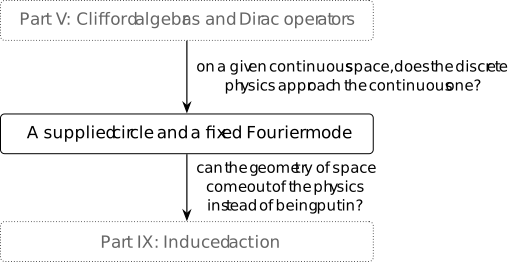
On a given continuous space, does the discrete physics approach the continuous one? The spatial Dirac calculation used lattice spacing one. Now supply a circle and place the graph on it. There are finitely many sites; the field values may still be real. For a field that changes over many vertices, the spacing is small relative to the scale of that change. Dividing an edge difference by the spacing then suggests a derivative. Continuous values concern the allowed field values, here real numbers; differentiability concerns the variation of a field on the supplied space and limits of difference quotients. Smoothness asks for derivatives of every order.
The circle calculation makes a limited comparison precise: each fixed Fourier mode of the discrete operator approaches its counterpart on the supplied circle. Approximation needs comparison maps and a limit; the chapter states these together with its pairings, positive precision and Gaussian moments. The circle is an input, so this result does not construct continuous space from the graph. The finite Dirac kernel in Proposition [fdip-000T] depends on the parity of the periods; that separate calculation cautions against inferring a general continuum theory from one fixed-mode limit. Whether continuous-space physics can be recovered at large scales without supplying the space remains open here.
1. A supplied circle and a fixed Fourier mode [fdip-004G]AGENTDRAFTED
- October 31, 2026
1. A supplied circle and a fixed Fourier mode [fdip-004G]AGENTDRAFTED
- October 31, 2026
How does a finite operator approximate a differential operator when the circle and its length are already given? A periodic mesh, a normalized pairing and a positive mass give an explicit answer for each fixed Fourier mode. The same calculation controls one Gaussian second moment, using normalization and inverse-precision covariance. The spatial Dirac comparison provides related finite symbols; the scalar argument below does not require its Clifford module.
Definition 1.1. A circle mesh with normalized pairing [fdip-004H]AGENTDRAFTED
- October 31, 2026
Definition 1.1. A circle mesh with normalized pairing [fdip-004H]AGENTDRAFTED
- October 31, 2026
Supply the unit circle \(\mathbb R/\mathbb Z\), its coordinate \(x\) modulo one and length measure \(dx\). For an integer \(n\geq 3\), the circle mesh consists of the points \(j/n\), with \(j\in \mathbb Z/n\mathbb Z\), and spacing \(h_n=1/n\). Its real field space and reference pairing are \[E_n=\mathbb R^{\mathbb Z/n\mathbb Z},\qquad g_{0,n}(f,g)=\frac 1n\sum _{j=0}^{n-1}f_jg_j.\] On the complexification use \(\langle f,g\rangle _n=n^{-1}\sum _j\overline {f_j}g_j\); its restriction to real fields is \(g_{0,n}\).
Fix a mass squared \(\mu >0\), independent of \(n\). Define the cyclic shift, scaled nearest-neighbor Laplacian and precision by \[\begin {aligned} (T_nf)_j&=f_{j+1},\\ L_n&=n^2(2I-T_n-T_n^{-1}),\\ Q_n&=\mu I+L_n,\qquad q_n(f)=g_{0,n}(f,Q_nf). \end {aligned}\] Indices are taken modulo \(n\). These specialize the cyclic shift and difference energy, with the supplied scale \(n^2\). The scalar \(L_n\) is the nearest-neighbor operator compared with, and generally different from, the centered Dirac square in Proposition [fdip-000T].
Periodic reindexing gives \(T_n^*=T_n^{-1}\) in the normalized pairing. Consequently \[\langle f,L_nf\rangle _n =n\sum _{j=0}^{n-1}|f_{j+1}-f_j|^2\geq 0.\] Thus \(Q_n\geq \mu I\) and \(Q_n\) is invertible, including on constant fields. This is the positive precision convention with the declared \(g_{0,n}\), rather than a change of the action form.
The step-function interpolation \(I_n\) assigns to \(f\) the function with value \(f_j\) whenever \(j/n\leq x<(j+1)/n\), using the representative \(0\leq x<1\). It maps real or complex fields into \(L^2(\mathbb R/\mathbb Z,dx)\), the square-integrable functions modulo almost-everywhere equality. Each interval has length \(1/n\), so \[\|I_nf\|_{L^2}^2=\frac 1n\sum _j|f_j|^2=\|f\|_n^2.\] Thus the comparison preserves the specified norm.
Example 1.2. Fourier modes and their Gaussian moments on a circle mesh [fdip-004I]AGENTDRAFTED
- October 31, 2026
Example 1.2. Fourier modes and their Gaussian moments on a circle mesh [fdip-004I]AGENTDRAFTED
- October 31, 2026
For the circle mesh, let \(k\in \mathbb Z\) and set \[e_k(x)=e^{2\pi ikx},\qquad e_{n,k}(j)=e^{2\pi ikj/n}.\] Every entry has modulus one, hence \(\|e_{n,k}\|_n=1\). Applying the shift and its inverse directly gives \[\begin {aligned} T_ne_{n,k}&=e^{2\pi ik/n}e_{n,k},\\ L_ne_{n,k}&=\lambda _{n,k}e_{n,k},\\ \lambda _{n,k} &=n^2(2-e^{2\pi ik/n}-e^{-2\pi ik/n})\\ &=4n^2\sin ^2(\pi k/n). \end {aligned}\] This derives the scaled version of the nearest-neighbor symbol. Frequencies differing by \(n\) give the same samples. For fixed \(k\ne 0\), the condition \(n>2|k|\) separates \(k\) from \(-k\) modulo \(n\).
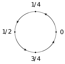
For \(k=0\), \(e_{n,0}=\mathbf 1\) and \(\lambda _{n,0}=0\). For \(k=1\), a four-point mesh has \(\lambda _{4,1}=32\); an eight-point mesh has \(\lambda _{8,1}=64(2-\sqrt 2)\). The picture shows the supplied unit circle sampled at 4 equally spaced points. Its arrows indicate increasing \(j\); they do not specify a dynamics.
Now use real fields and the Gaussian law \[d\nu _n(f)=Z_n^{-1}e^{-q_n(f)/2}\,d\operatorname {vol}_{g_{0,n}}(f).\] In raw coordinates the volume and normalization are \[\begin {aligned} d\operatorname {vol}_{g_{0,n}}&=n^{-n/2}\,df_0\cdots df_{n-1},\\ Z_n&=(2\pi )^{n/2}(\det Q_n)^{-1/2}. \end {aligned}\] The volume factor follows because \(f\mapsto f/\sqrt n\) is an orthonormal chart; the partition function is Theorem [fdip-002T]. The covariance operator relative to \(g_{0,n}\) is \(Q_n^{-1}\) by Theorem [fdip-000B]. Since the exponent is \(f^TQ_nf/(2n)\), the raw coordinate covariance matrix is \(nQ_n^{-1}\).
Define the complex Fourier observable \(a_{n,k}=n^{-1}\sum _j e^{-2\pi ikj/n}f_j\). It has zero mean. Writing \(v=e_{n,k}\) and \(v^*\) for its conjugate transpose, the coordinate covariance gives \[\begin {aligned} \mathbb E_{\nu _n}|a_{n,k}|^2 &=n^{-2}v^*(nQ_n^{-1})v\\ &=\frac 1{\mu +\lambda _{n,k}}, \end {aligned}\] because \(v^*v=n\). All real and imaginary parts and their products are integrable polynomials by Proposition [fdip-002W]. In particular the real mean \(a_{n,0}\) has variance \(1/\mu \). At \(k=1\), the four-point and eight-point second moments are respectively \((\mu +32)^{-1}\) and \((\mu +64(2-\sqrt 2))^{-1}\).
For \(k\ne 0\) and \(n>2|k|\), put \[\begin {aligned} c_{n,k}&=\operatorname {Re}a_{n,k} =\frac 1n\sum _j\cos (2\pi kj/n)f_j,\\ s_{n,k}&=-\operatorname {Im}a_{n,k} =\frac 1n\sum _j\sin (2\pi kj/n)f_j. \end {aligned}\] The geometric sum \(\sum _j e^{4\pi ikj/n}=0\): its ratio is not one, its \(n\)-th power is one, and multiplying the sum by one minus the ratio gives zero. Taking real and imaginary parts, and using the double-angle identities, gives normalized squared norms \(1/2\) for both the cosine and sine vectors and their orthogonality. Both vectors have precision eigenvalue \(\mu +\lambda _{n,k}\), so Theorem [fdip-000B] yields \[\operatorname {Var}(c_{n,k})=\operatorname {Var}(s_{n,k}) =\frac 1{2(\mu +\lambda _{n,k})}.\] The coefficients of the orthogonal projection \(A\cos (2\pi kj/n)+B\sin (2\pi kj/n)\) are \(A=2c_{n,k}\), \(B=2s_{n,k}\). Their variances are 4 times the displayed projection variances.
The character calculation and normalization above are direct
deductions from the cited finite operators and Gaussian results.
Mathlib's ZMod.dft uses the counting-measure forward sum;
\(a_{n,k}\) has the additional factor \(1/n\). This formal Fourier
transform is a supporting construction, not a formalization of the
mesh limit.
Proposition 1.3. A fixed Fourier mode and its massive inverse converge [fdip-004J]AGENTDRAFTED
- October 31, 2026
Proposition 1.3. A fixed Fourier mode and its massive inverse converge [fdip-004J]AGENTDRAFTED
- October 31, 2026
Use the circle meshes with fixed \(\mu >0\), and fix \(k\in \mathbb Z\) before letting \(n\to \infty \). For the Fourier modes and eigenvalues, \[\begin {aligned} \lambda _{n,k}&\longrightarrow 4\pi ^2k^2,\\ (\mu +\lambda _{n,k})^{-1} &\longrightarrow (\mu +4\pi ^2k^2)^{-1}. \end {aligned}\] Moreover, in \(L^2(\mathbb R/\mathbb Z,dx)\), \[I_nQ_n^{-1}e_{n,k} \longrightarrow (\mu +4\pi ^2k^2)^{-1}e_k.\] The vector on the right solves \(Au=e_k\) for \(A=-d^2/dx^2+\mu \) on smooth periodic functions. The selected Gaussian moment \(\mathbb E_{\nu _n}|a_{n,k}|^2\) converges to the same inverse eigenvalue.
Proof.
- October 31, 2026
Proof.
- October 31, 2026
For \(k=0\), the eigenvalue is identically zero and the sampled constant interpolates exactly to \(e_0=1\); all three assertions follow. For \(k\ne 0\), \[\lambda _{n,k} =4\pi ^2k^2\left (\frac {\sin (\pi k/n)}{\pi k/n}\right )^2.\] The sine quotient tends to one. Since \(\mu >0\), all denominators are at least \(\mu \), so continuity of inversion proves the scalar inverse limit.
For \(j/n\leq x<(j+1)/n\), the elementary inequality \(|e^{it}-e^{is}|\leq |t-s|\) gives \[|I_ne_{n,k}(x)-e_k(x)|\leq \frac {2\pi |k|}{n}.\] The inequality follows by integrating \(ie^{iu}\) between \(s\) and \(t\). The circle has measure one, hence the same bound holds for the \(L^2\) norm. Put \(b_n=(\mu +\lambda _{n,k})^{-1}\) and \(b=(\mu +4\pi ^2k^2)^{-1}\). Because \(|b_n|\leq 1/\mu \) and \(\|e_k\|_{L^2}=1\), \[\begin {aligned} \|b_nI_ne_{n,k}-be_k\|_{L^2} &\leq |b_n|\|I_ne_{n,k}-e_k\|_{L^2}+|b_n-b|\\ &\leq \frac {2\pi |k|}{\mu n}+|b_n-b|\longrightarrow 0. \end {aligned}\] The eigenvector equation identifies the left vector with \(I_nQ_n^{-1}e_{n,k}\). Differentiation gives \(Ae_k=(\mu +4\pi ^2k^2)e_k\). Finally the Gaussian second-moment formula in Example 1.2 is exactly \(b_n\).
This is an elementary limit deduction from the preceding finite
symbol, with an explicit interpolation map. Mathlib's
Real.tendsto_sin_div_nhdsNE_zero supplies the nonzero
sine-quotient limit used in the proof; the zero mode was handled
separately. The declaration does not supply the interpolation or
Gaussian comparison.
Remark 1.4. What the supplied-circle limit establishes [fdip-004K]AGENTDRAFTED
- October 31, 2026
Remark 1.4. What the supplied-circle limit establishes [fdip-004K]AGENTDRAFTED
- October 31, 2026
The fixed-mode limit compares finite operators and one Gaussian moment with a declared circle. Its length, measure, mesh spacing, factor \(n^2\) and positive mass are supplied. Without \(n^2\), each fixed-mode Laplacian eigenvalue tends to zero. This explains why a finite positive operator alone does not determine a continuum scale or geometry.
The quantifier on the frequency matters. For even \(n\) and \(k=n/2\), the discrete eigenvalue is \(4n^2\), whereas the continuum frequency has eigenvalue \(4\pi ^2k^2=\pi ^2n^2\). Their ratio stays \(4/\pi ^2\); the fixed-mode proof is therefore not a relative uniform estimate over all modes. It proves neither operator-norm resolvent convergence nor convergence of determinants or Gaussian measures. Removing the positive mass or adding interactions requires additional arguments.
For comparison, Weisz distinguishes the critical-point and phase-diagram control needed for low-energy lattice-QCD continuum limits from the renormalization questions for composite observables and high-energy scales [weisz2010renormalization, Section 1.1, printed p. 2]. The circle calculation is a much smaller prescribed approximation: it contains no interacting critical-point analysis. It establishes no emergent geometry, reflection positivity, Lorentzian reconstruction, Standard Model dynamics or gravitational dynamics. Those identifications remain among the open physical interfaces.