Group-algebra sectors [fdip-001A]
✍️sourceAGENTDRAFTED
- October 20, 2026
Group-algebra sectors [fdip-001A]
✍️sourceAGENTDRAFTED
- October 20, 2026
How can the same half-turn act on different Gaussian states? The group-algebra extension and its module projectors separate the actual half-turn sectors whenever two is invertible. The action and its projectors are specified before a probability law is attached. Support parity and sign sectors are different decompositions of the same fields.
Over the reals, an orthogonal involution commuting with positive precision gives a product law; the four-cycle calculation computes its two blocks and retained marginals. Symmetry still permits mixing within a sector, and in characteristic two the action survives without the complementary projectors. These examples separate the supplied symmetry, the coefficient assumptions and the choice of state.
Theorem 1. Extending a group action on a ring module [fdip-003N]AGENTDRAFTED
- October 29, 2026
Theorem 1. Extending a group action on a ring module [fdip-003N]AGENTDRAFTED
- October 29, 2026
Let \(k\) be a commutative unital ring, \(G\) a group and \(M\) a unital \(k\)-module. A linear action \(\rho :G\to \operatorname {Aut}_k(M)\) extends uniquely to a unital \(k\)-algebra homomorphism \[\widehat \rho :k[G]\longrightarrow \operatorname {End}_k(M),\qquad \widehat \rho \left (\sum _g a_g[g]\right )=\sum _g a_g\rho (g).\] Products of endomorphisms compose right to left. This extends the Group Algebra universal property to the actual module action; no finiteness of \(G\) is assumed.
Proof.
- October 29, 2026
Proof.
- October 29, 2026
Elements of \(k[G]\) are finite-support functions on \(G\). The coefficient of \([u]\) in a product is \(\sum _{gh=u}a_gb_h\); only pairs in the finite set \(\operatorname {supp}(a)\times \operatorname {supp}(b)\) contribute. Its image under multiplication contains the product support. Associativity follows by reassociating the finite triple sum and using \((gh)j=g(hj)\). The unit is \([1_G]\), and the scalar \(c[1_G]\) commutes with every basis element. Thus these formulas define a unital \(k\)-algebra, including for the zero ring.
The displayed extension is additive and \(k\)-linear. Moreover \[\begin {aligned} \widehat \rho (ab)&=\sum _{g,h}a_gb_h\rho (gh)\\ &=\sum _{g,h}a_gb_h\rho (g)\rho (h) =\widehat \rho (a)\widehat \rho (b). \end {aligned}\] The \(k\)-linearity of each \(\rho (g)\) moves coefficients through it; the order of \(g,h\) is unchanged. The extension sends \([1_G]\) to \(I_M\) and \(c[1_G]\) to \(cI_M\). Every linear extension has this value on each finite basis expansion, proving uniqueness. In the regular action, \(\rho (g)\rho (h)\) first multiplies \([1_G]\) by \([h]\), then by \([g]\), giving \([gh]\). For \(g=(12),h=(23)\) in \(S_3\), this differs from \([hg]\) when \(k\ne 0\). The nonzero assumption is needed only for this distinguishing witness.
Consequently linear \(G\)-actions correspond to unital left \(k[G]\)-module structures whose restriction along \(c\mapsto c[1_G]\) is the given scalar action. Under this correspondence, a \(k\)-linear map \(f:M\to N\) is a module map exactly when \(f\rho _M(g)=\rho _N(g)f\) for every \(g\).
Proof.
- October 29, 2026
Proof.
- October 29, 2026
Define \(a\cdot m=\widehat \rho (a)m\); linearity, multiplication and the unit just proved give the module laws. Conversely, restrict a \(k[G]\)-module to \(k\) and set \(\rho (g)m=[g]m\). Centrality of scalars gives \(k\)-linearity, \([g^{-1}]\) gives the inverse, and \([gh]=[g][h]\) gives the representation law. Finite distributivity shows that the two constructions are inverse. This scalar restriction is essential; an unrelated \(k\)-module structure is not being identified.
If \(f\) intertwines the group elements, finite linearity gives \[f\widehat \rho _M(a)m =\sum _g a_g f\rho _M(g)m =\sum _g a_g\rho _N(g)fm =\widehat \rho _N(a)fm.\] The converse follows by taking \(a=[g]\). This proves intertwining for every algebra element, including scalars and the unit.
[sengupta2010representations, Sections 3.1-3.2, pp. 39-41]
presents the field case, with finite support for an arbitrary group.
The proof above is the ring adaptation of
representation/module correspondence.
Mathlib's Representation.asAlgebraHom and
Representation.asAlgebraHom_single supply the linear extension
and its value on basis monomials. They do not assert that an arbitrary
faithful group action has a faithful algebra extension. For example,
\(C_2\to \mathbb R^\times \), \(r\mapsto -1\), is injective, but its
algebra extension annihilates the nonzero element \(1+[r]\).
Theorem 2. Projectors of an involution on a module [fdip-003O]AGENTDRAFTED
- October 29, 2026
Theorem 2. Projectors of an involution on a module [fdip-003O]AGENTDRAFTED
- October 29, 2026
Let \(k\) be a commutative unital ring in which \(2\) is a unit, put \(h=2^{-1}\), and let \(T:M\to M\) be linear with \(T^2=I\). The maps \(E_\varepsilon =h(I+\varepsilon T)\), for \(\varepsilon \in \{1,-1\}\), give \[\begin {aligned} E_\varepsilon ^2&=E_\varepsilon ,&E_+E_-&=E_-E_+=0,\\ E_++E_-&=I,&E_+-E_-&=T,\\ \operatorname {im}E_\varepsilon &=\ker (T-\varepsilon I)=M_\varepsilon . \end {aligned}\] Thus \(M\cong M_+\oplus M_-\), with map \(v\mapsto (E_+v,E_-v)\) and inverse addition. No finite generation, freeness or pairing is needed.
Proof.
- October 29, 2026
Proof.
- October 29, 2026
Scalar maps commute with \(T\), so \[E_\varepsilon ^2=h^2(I+2\varepsilon T+T^2) =2h^2(I+\varepsilon T)=E_\varepsilon .\] Both mixed products equal \(h^2(I-T^2)=0\); sum and difference use \(2h=1\). Also \(TE_\varepsilon =\varepsilon E_\varepsilon \). If \(Tv=\varepsilon v\), then \(E_\varepsilon v=h(v+v)=v\), proving equality of image and eigenspace. The sum identity decomposes every vector. If \(u_++u_-=0\) with \(u_\pm \in M_\pm \), applying \(E_+\) gives \(u_+=0\), and then \(u_-=0\), proving uniqueness.
If an algebra acts by \(\alpha :A\to \operatorname {End}_k(M)\), these projectors are \(A\)-linear precisely when \[T\alpha (a)=\alpha (a)T\qquad (a\in A).\] Indeed this is exactly \(A\)-linearity of \(T\); its linear combinations with \(I\) are then \(A\)-linear. Conversely, either projector recovers \(T=2E_+-I=I-2E_-\). When \(T=\alpha (\omega )\), centrality of \(\omega \) is sufficient. It need not be necessary: on \(M=\mathbb R\), let \(A=\mathbb R\times M_2(\mathbb R)\) act by \(\alpha (a,B)=aI\), and put \(\omega =(1,\operatorname {diag}(1,-1))\). Then \(\omega ^2=1\) and \(T=I\), although \(\omega \) fails to commute with a matrix unit in the second factor.
For comparison, the central-idempotent product is an algebra statement. Central orthogonal idempotents \(e_+,e_-\) with sum one give the mutually inverse unital algebra maps \[a\longmapsto (e_+a,e_-a),\qquad (x,y)\longmapsto x+y.\] Each ideal \(e_\varepsilon A\) has unit \(e_\varepsilon \) and scalar map \(c\mapsto ce_\varepsilon \). Centrality makes each component multiplicative and the mixed products zero; the sum and orthogonality identities prove both inverse equations. This is stronger than the module splitting above.
In \(k[C_2]\), writing \(g=[r]\) for \(r^2=1\), the two central idempotents are \(e_\pm =h(1\pm g)\). The explicit product is \[\begin {aligned} \Phi (a+bg)&=(a+b,a-b),\\ \Phi ^{-1}(x,y)&=h(x+y)+h(x-y)g. \end {aligned}\] The coefficient product \((a+bg)(c+dg)=(ac+bd)+(ad+bc)g\) maps to \(((a+b)(c+d),(a-b)(c-d))\). Thus \(\Phi \) is multiplicative; its inverse equations use \(2h=1\), its unit image is \((1,1)\), and scalars map diagonally. The images of \(e_+,e_-\) are \((1,0),(0,1)\). An arbitrary coefficient ring need not be semisimple, and an abstract idempotent summand need not be free.
[sengupta2010representations, Section 4.5, pp. 63-64]
discusses character projectors over a field with invertible group order;
its subsequent ideal argument assumes semisimplicity. The displayed
ring identities require only invertible two. Mathlib's
LinearMap.IsIdempotentElem.isCompl supplies the abstract
range/kernel complement. TauCeti's
TauCeti.isIdempotentElem_halfOneAdd supplies the
square-one idempotent identity, and
MonoidAlgebra.cyclicTwoEquivProd supplies the
\(C_2\) algebra product. Its generator is
\(\operatorname {Multiplicative.ofAdd}(1:\mathbb Z/2\mathbb Z)\).
None of these facts determines the ranks of a particular represented
sector; those require the coordinate bases.
Definition 3. The group-algebra action of the half-turn [fdip-000L]AGENTDRAFTED
- October 17, 2026
Definition 3. The group-algebra action of the half-turn [fdip-000L]AGENTDRAFTED
- October 17, 2026
The half-turn acts on fields before a precision or probability law is chosen. Let \(k\) be a nonzero commutative ring and \(C_2=\{1,r\}\), with \(r^2=1\). In its Group Algebra, write \(g=[r]\) and \(1=[1]\). Every element has unique coefficients \(a+bg\), and \[\begin {aligned} (a+bg)(c+dg)&=(ac+bd)\\ &\quad +(ad+bc)g. \end {aligned}\] [sengupta2010representations, Sections 3.1-3.2, pp. 39-41] gives the group basis and linear extension over a field. The ring-module extension supplies the general ring theorem; the following formulas identify its particular faithful actions.
Put \(V_k=k^4\), in vertex order \((0,1,2,3)\), and \(W_k=k^R\), with \(R=(0,2)\) in that order. Let \(\delta _i(j)=\mathbf 1_{j=i}\) be the coordinate basis of \(V_k\); let \(\delta _i^R(j)=\mathbf 1_{j=i}\) for \(i,j\in R\) be the coordinate basis of \(W_k\). These coordinate vectors differ from the real spectral vectors \(u_a\) and from the edge labels \(e_i\). The half-turn and its retained action are \[\begin {aligned} P(\phi _0,\phi _1,\phi _2,\phi _3)&=(\phi _2,\phi _3,\phi _0,\phi _1),\\ J(x_0,x_2)&=(x_2,x_0). \end {aligned}\] Applying either permutation twice returns the original coordinates, so \(P^2=I\) and \(J^2=I\). Their unique unital \(k\)-algebra extensions are \[\begin {aligned} \widehat \rho _V:k[C_2]&\longrightarrow \operatorname {End}_k(V_k),\\ \widehat \rho _V(a+bg)&=aI+bP,\\ \widehat \rho _W:k[C_2]&\longrightarrow \operatorname {End}_k(W_k),\\ \widehat \rho _W(a+bg)&=aI+bJ. \end {aligned}\] The associated left module action is \(z\cdot v=\widehat \rho _V(z)v\), and similarly on \(W_k\). Both algebra actions are faithful, meaning that their defining maps are injective.
Indeed, \(P^2=I\) gives \[\begin {aligned} (aI+bP)(cI+dP) &=(ac+bd)I\\ &\quad +(ad+bc)P. \end {aligned}\] The same calculation uses \(J^2=I\) on \(W_k\). Addition and scalar multiplication are preserved term by term, and \(1\) maps to \(I\). These facts prove the module laws. A linear extension is unique because \(1,g\) are a basis. If \(aI+bP=0\), applying it to \(\delta _0\) gives \(a\delta _0+b\delta _2=0\); coordinates \(0,2\) give \(a=b=0\). Applying \(aI+bJ\) to \(\delta _0^R\) proves injectivity on \(W_k\) in the same way. No absence of zero divisors is required.
Coordinate projection \(\pi _R(\phi )=(\phi _0,\phi _2)\) sends \(\delta _0,\delta _2\) to \(\delta _0^R,\delta _2^R\) and kills \(\delta _1,\delta _3\). Since \(\pi _RP=J\pi _R\), it intertwines the whole algebra action: \[\pi _R\widehat \rho _V(z)=\widehat \rho _W(z)\pi _R \qquad (z\in k[C_2]).\] Thus it is a \(k[C_2]\)-module map by the all-element intertwining theorem. Both coordinate faithfulness witnesses above work with zero divisors; they use more than faithfulness of the group action alone.
Suppose now that \(2\) is a unit in \(k\), and put \(h=2^{-1}\). The element \(g\) is a central involution. Its two idempotents and algebra product are \[e_+=h(1+g),\qquad e_-=h(1-g).\] Their images under the two algebra actions are the following concrete module projectors. Abstract centrality in \(k[C_2]\) supplies commutation with the represented algebra; it does not make \(P\) central in all \(\operatorname {End}_k(V_k)\).
The represented projectors are \[E_\pm =h(I\pm P),\qquad F_\pm =h(I\pm J).\] They give the eigenspace decompositions \[\begin {aligned} V_k&=V_+\oplus V_-,&V_\pm &=\operatorname {im}E_\pm ,\\ W_k&=W_+\oplus W_-,&W_\pm &=\operatorname {im}F_\pm . \end {aligned}\] For either sign \(\varepsilon \in \{1,-1\}\), the concrete half-turn sector is \[\begin {aligned} V_\varepsilon &=\{(x,y,\varepsilon x,\varepsilon y):x,y\in k\},\\ W_\varepsilon &=\{(x,\varepsilon x):x\in k\}. \end {aligned}\] Their free bases are \[\begin {aligned} b_{\varepsilon ,0}&=\delta _0+\varepsilon \delta _2,\\ b_{\varepsilon ,1}&=\delta _1+\varepsilon \delta _3,\\ c_\varepsilon &=\delta _0^R+\varepsilon \delta _2^R. \end {aligned}\] The first two coordinates of \(V_\varepsilon \), and the first coordinate of \(W_\varepsilon \), recover the coefficients uniquely. Consequently the free ranks are two and one.
To verify the splitting, \(E_++E_-=I\) gives
\(v=E_+v+E_-v\). An element in both images is fixed and annihilated
by \(E_+\), so it is zero. Further, \(PE_\varepsilon =\varepsilon
E_\varepsilon \), while \(Pv=\varepsilon v\) gives
\(E_\varepsilon v=h(v+\varepsilon Pv)=v\). This identifies the
images with the displayed coordinate sets; the proof for \(W_k\) is
identical. Mathlib's LinearMap.IsIdempotentElem.isCompl
supplies the abstract complement between an idempotent's range and
kernel. The coordinate bases and ranks above identify its concrete
summands here.
Projection respects these summands: \[\pi _RE_\varepsilon =F_\varepsilon \pi _R.\] Its restriction \(\pi _\varepsilon :V_\varepsilon \to W_\varepsilon \) sends \(b_{\varepsilon ,0}\) to \(c_\varepsilon \) and \(b_{\varepsilon ,1}\) to zero. It is surjective, with \[\ker \pi _\varepsilon =k b_{\varepsilon ,1}.\] The first coefficient of a sector vector proves the kernel formula and the displayed image of \(b_{\varepsilon ,0}\) proves surjectivity. For each sign, the square commutes, with the horizontal codomains restricted to the indicated sectors:
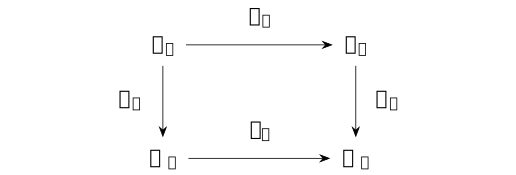
The horizontal maps select a sector; the right map removes one free coordinate within it. The algebra factors \(k\times k\), the full rank-two sectors, and the retained rank-one sectors are different levels of decomposition.
Remark 4. Support parity, group degree and sign sectors [fdip-003P]AGENTDRAFTED
- October 29, 2026
Remark 4. Support parity, group degree and sign sectors [fdip-003P]AGENTDRAFTED
- October 29, 2026
For the four-cycle over a nonzero commutative ring with invertible two, three decompositions record different structures. The support grading separates fields supported on \(\{0,2\}\) and \(\{1,3\}\). The one-step shift \(Tf(i)=f(i+1)\) exchanges these supports, so it is odd, whereas \(P=T^2\) and \(E_\pm =h(I\pm P)\) preserve them and are even. A single half-turn sign sector contains both \(b_{\varepsilon ,0}=\delta _0+\varepsilon \delta _2\) and \(b_{\varepsilon ,1}=\delta _1+\varepsilon \delta _3\), which have different support parities. A minus eigenvalue does not mean odd support.
The canonical group grading of \(k[C_2]\) has components \(k\,1\) of degree \(1_G\) and \(k\,g\) of degree \(r\). Their multiplication follows the group law, in particular \(g^2=1\). Over a ring these are rank-one free summands. The representation sends \(g\) to support-even \(P\); it therefore does not preserve these particular gradings under \(r\mapsto 1\in \mathbb Z/2\mathbb Z\). The projector ideals are different again: \(e_-^2=e_-\ne 0\), while an odd homogeneous component would have its square in the even component. The direct product, the group grading and the support grading cannot be interchanged. These are the distinct splitting levels applied to the concrete action.
The ordinary adjoint uses the counting pairing \(b(f,u)=\sum _i f_i u_i\), with identity coefficient involution. Delta vectors recover all coefficients, so the pairing is perfect. Reindexing a finite sum shows that every permutation action is an isometry, hence \[b(\rho (\sigma )f,u)=b(f,\rho (\sigma ^{-1})u).\] Uniqueness of the ordinary adjoint gives \(\rho (\sigma )^\dagger =\rho (\sigma ^{-1})\); in particular \(T^\dagger =T^{-1}\) and \(P^\dagger =P\). There is no complex conjugation or Koszul sign in this calculation.
The corresponding ordinary group-algebra operation is \[\left (\sum _g a_g[g]\right )^*=\sum _g a_g[g^{-1}].\] It is \(k\)-linear, fixes scalars, squares to the identity and reverses products, since \((gh)^{-1}=h^{-1}g^{-1}\) and all sums are finite. For an isometric representation with a perfect pairing, taking the adjoint of its finite linear extension therefore gives \(\widehat \rho (z^*)=\widehat \rho (z)^\dagger \). The isometry premise matters: the infinite cyclic group acting on \(\mathbb R\) by multiplication by \(2\) has adjoint \(2\) and inverse \(1/2\), so this identity fails for that representation. The counting action satisfies the premise.
The group basis and inversion are as in [sengupta2010representations, Sections 3.1-3.2, pp. 39-41]; the grading and adjoint comparisons above are direct calculations. The shift calculation supplies the support-degree and adjoint identities. Clifford parity of a quadratic quotient is a further structure; these ordinary formulas introduce neither a graded star nor a Hermitian extension.
Theorem 5. The real Gaussian law is a product over orthogonal sectors [fdip-000M]AGENTDRAFTED
- October 17, 2026
Theorem 5. The real Gaussian law is a product over orthogonal sectors [fdip-000M]AGENTDRAFTED
- October 17, 2026
Let \(H\) be a finite-dimensional real inner-product space, \(P:H\to H\) an orthogonal involution, and \(Q:H\to H\) a positive self-adjoint precision with \(QP=PQ\). Put \(H_\varepsilon =\ker (P-\varepsilon I)\) and \(E_\varepsilon =(I+\varepsilon P)/2\). Use induced Euclidean volumes on the uncompleted Borel sigma-algebras. The restrictions \(Q_\varepsilon =Q|_{H_\varepsilon }\) are positive self-adjoint. For their Gaussian laws, \[\begin {aligned} D:H&\longrightarrow H_+\times H_-,\\ z&\longmapsto (E_+z,E_-z),\\ D_*\mu _Q&=\mu _{Q_+}\otimes \mu _{Q_-},\qquad Z_Q=Z_{Q_+}Z_{Q_-}. \end {aligned}\] Thus the sector-valued random variables \(E_+,E_-\) are independent with the indicated marginal laws. The four-cycle recovery computes both blocks, their normalizers and their retained scalar laws explicitly.
Proof.
- October 17, 2026
Proof.
- October 17, 2026
The module projector identities give the direct sum. For \(u\in H_+\), \(v\in H_-\), orthogonality of \(P\) gives \(\langle u,v\rangle =\langle Pu,Pv\rangle =-\langle u,v\rangle \), so \(\langle u,v\rangle =0\). Addition \(J:H_+\times H_-\to H\), \(J(u,v)=u+v\), is therefore an isometric linear isomorphism with inverse \(D\). Commutation gives \(PQu=QPu=\varepsilon Qu\) for \(u\in H_\varepsilon \); hence \(Q\) preserves each sector. Restricting its pairing identity and testing nonzero sector vectors proves self-adjointness and positivity of \(Q_\varepsilon \).
Concatenating orthonormal bases of \(H_+,H_-\) gives an orthonormal basis of \(H\). Coordinate product Lebesgue measure, transported by these charts, therefore proves \[J_*(\lambda _+\otimes \lambda _-)=\lambda _H,\qquad D_*\lambda _H=\lambda _+\otimes \lambda _-.\] This is precisely orthogonal product volume. Finite-dimensional spaces have countable bases, so the product Borel sigma-algebra is the Borel sigma-algebra of the product. Bounded coordinate cubes exhaust each space, proving sigma-finiteness. A zero-dimensional sector has unit mass on its sole point.
Orthogonality and preservation of sectors give the action identity \[\langle u+v,Q(u+v)\rangle =\langle u,Q_+u\rangle +\langle v,Q_-v\rangle .\] For \(w_Q(z)=e^{-\langle z,Qz\rangle/2}\), this says \(w_Q(J(u,v))=w_{Q_+}(u)w_{Q_-}(v)\). The positive normalizer theorem applies separately to all three positive self-adjoint maps: \[Z_R=\frac {(2\pi )^{\dim U/2}}{\sqrt {\det R}}\in (0,\infty ) \quad (R=Q,Q_+,Q_-\text { on its space }U).\] Its proof uses positive eigenvalues, the scalar Gaussian integral and nonnegative Tonelli, without presupposing this product law. Empty determinants and normalizers are one. Applying Tonelli with the volume and weight identities just proved gives \(Z_Q=Z_{Q_+}Z_{Q_-}\).
For Borel sets \(A_+\subseteq H_+\), \(A_-\subseteq H_-\), all the following integrands are nonnegative measurable functions: \[\begin {aligned} (D_*\mu _Q)(A_+\times A_-) &=\frac {1}{Z_{Q_+}Z_{Q_-}}\\ &\quad \cdot \int _{A_+\times A_-}w_{Q_+}(u)w_{Q_-}(v) \,d(\lambda _+\otimes \lambda _-)(u,v)\\ &=\mu _{Q_+}(A_+)\mu _{Q_-}(A_-). \end {aligned}\] Rectangles form a pi-system containing the whole product and generating its Borel sigma-algebra. The pi-lambda uniqueness theorem for finite measures identifies the two probability measures everywhere. Their coordinate marginals and the displayed rectangle equation are exactly independence of \(E_+,E_-\). The argument also covers a zero sector, whose law is deterministic. Algebraic splitting alone would not have supplied this probability identity.
For the actual polynomial function algebras, write \(\omega _R(p)=\int p\,d\mu _R\). Then \[\omega _Q\bigl ((p_+\circ E_+)(p_-\circ E_-)\bigr ) =\omega _{Q_+}(p_+)\omega _{Q_-}(p_-).\] Indeed linear precomposition takes polynomial generators to polynomial generators. Every polynomial, product and square has finite absolute Gaussian integral by Proposition [fdip-002W], applied on the full space and on each sector. Tonelli applied first to the absolute product therefore justifies signed Fubini, which gives the formula from the product law. These are real polynomial states: they are linear, normalized and nonnegative on \(p^2\), with the identity star. No algebra structure on all integrable functions, or state on \(\operatorname {End}(H)\), is being used.
[friedli2017statistical, Proposition B.55, p. 505] uses covariance as its positive parameter. In an orthonormal chart, set \(\Sigma =Q^{-1}\). Its eigenvalues are positive, \(\Sigma ^{-1}=Q\) and \(\det \Sigma =(\det Q)^{-1}\), so its normalized density is exactly \(Z_Q^{-1}w_Q\). The inverse-precision covariance theorem identifies \(\Sigma \) as the covariance. The product proof above uses densities, not an inference from zero covariance for an unspecified law.
Mathlib's OrthonormalBasis.measurePreserving_repr
supports passage to orthonormal coordinates. Index coordinates by the
disjoint union of orthonormal bases of \(H_+\) and \(H_-\). Then
\(\Sigma =\operatorname {diag}(Q_+^{-1},Q_-^{-1})\) is positive
definite, hence positive semidefinite, with zero cross block and mean
zero. After the density identification, TauCeti's
TauCeti.Probability.indepFun_sumEquivProd_multivariateGaussian_iff
gives the corresponding coordinate independence. It concerns this
Gaussian covariance, not an arbitrary algebraic splitting or Schur
fiber integral.
The integration convention is [tao2011measure, Theorem 1.7.15, pp. 200-201, preliminary version]. All probability assertions here are finite-dimensional and real, with strictly positive precision and specified volume. They supply no Lebesgue probability over a general coefficient ring; a singular precision needs a separately specified constrained space and law.
Proposition 6. Restricting a split Schur map to sign sectors [fdip-003Q]AGENTDRAFTED
- October 29, 2026
Proposition 6. Restricting a split Schur map to sign sectors [fdip-003Q]AGENTDRAFTED
- October 29, 2026
Let \(k\) be a commutative unital ring with invertible two and \(H=X\oplus Y\). Let \(P=P_X\oplus P_Y\), where \(P_X^2=I_X\), \(P_Y^2=I_Y\), and let \(Q:H\to H\) commute with \(P\). Write the typed split components as \[\begin {aligned} A&:X\to X,&B&:Y\to X,\\ E&:X\to Y,&C&:Y\to Y,\\ Q(x,y)&=(Ax+By,Ex+Cy). \end {aligned}\] If \(C\) is invertible, the split Schur map \(S=A-BC^{-1}E\) preserves both sign sectors of \(P_X\), and \[S|_{X_\varepsilon } =A_\varepsilon -B_\varepsilon C_\varepsilon ^{-1}E_\varepsilon .\] Here \(X_\varepsilon =\ker (P_X-\varepsilon I)\), \(Y_\varepsilon =\ker (P_Y-\varepsilon I)\), and each subscript means restriction to the indicated source and target sectors.
Proof.
- October 29, 2026
Proof.
- October 29, 2026
Evaluate \(QP=PQ\) on \((x,0)\) and \((0,y)\) and project to both summands. This gives \[\begin {aligned} AP_X&=P_XA,&BP_Y&=P_XB,\\ EP_X&=P_YE,&CP_Y&=P_YC. \end {aligned}\] Multiplying the last identity on both sides by the inverse of \(C\) gives \(C^{-1}P_Y=P_YC^{-1}\). Each of these identities proves that its map takes sign-\(\varepsilon \) vectors to sign-\(\varepsilon \) vectors. In particular \(C_\varepsilon \) is invertible, with inverse \(C^{-1}|_{Y_\varepsilon }\), since the two inverse equations restrict to the sector. Finally \[\begin {aligned} SP_X&=AP_X-BC^{-1}EP_X\\ &=P_XA-BP_YC^{-1}E=P_XS. \end {aligned}\] Restricting the actual composite \(BC^{-1}E:X\to X\) now gives exactly the asserted formula, with no interchange of differently typed factors.
This is the sign-sector specialization of Schur transport, using the module projectors. Its block convention agrees with [boyd2004convex, Appendix A.5.5, pp. 650-651] after exchanging the source's first pivot to \(C\). The proof here is over modules; no pairing, self-adjointness, stationary field or probability law has been assumed. If the prescribed splitting is not preserved by \(P\), the required \(P_X,P_Y\) and these restrictions are not supplied.
Theorem 7. Gaussian marginalization commutes with sector decomposition [fdip-003R]AGENTDRAFTED
- October 29, 2026
Theorem 7. Gaussian marginalization commutes with sector decomposition [fdip-003R]AGENTDRAFTED
- October 29, 2026
Let \(H=X\mathbin \perp Y\) be a finite-dimensional real orthogonal sum, \(P=P_X\oplus P_Y\) an orthogonal involution, and \(Q\) a positive self-adjoint precision commuting with \(P\). Use induced Euclidean volumes and Borel Gaussian laws. For \(Q(x,y)=(Ax+By,B^\dagger x+Cy)\), put \(S=A-BC^{-1}B^\dagger \). The sign sectors are \(H_\varepsilon =X_\varepsilon \mathbin \perp Y_\varepsilon \). Let \(\pi (x,y)=x\) and let \(\pi _\varepsilon \) be its sector restriction. The typed restriction identity gives \[S_\varepsilon :=S|_{X_\varepsilon } =A_\varepsilon -B_\varepsilon C_\varepsilon ^{-1} B_\varepsilon ^\dagger .\] Then the following square commutes both for maps and for their pushforwards of the Gaussian laws:
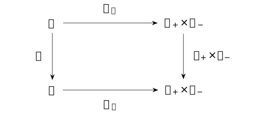
Here \(D_H(z)=(E_+z,E_-z)\) and \(D_X(x)=(F_+x,F_-x)\) are the orthogonal sector decompositions. The full retained law is \(\pi _*\mu _Q=\mu _S\); both routes give \(\mu _{S_+}\otimes \mu _{S_-}\) on \(X_+\times X_-\).
Proof.
- October 29, 2026
Proof.
- October 29, 2026
Testing positivity on \((0,y)\) makes \(C\) positive and invertible. Its inverse is self-adjoint by adjointing both inverse equations, so \(S\) is self-adjoint. With \(K=C^{-1}B^\dagger \), expansion gives \[\langle (x,y),Q(x,y)\rangle =\langle x,Sx\rangle +\langle y+Kx,C(y+Kx)\rangle .\] The two cross terms sum to \(2\langle x,By\rangle \); the last \(K\)-term cancels the subtraction in \(S\). Testing on \((x,-Kx)\) proves \(S>0\). Thus the hypotheses of positive Gaussian elimination hold. For every fixed \(x\), translation by \(Kx\) preserves induced volume, giving the pointwise fiber identity \[\int _Y e^{-\langle (x,y),Q(x,y)\rangle/2}\,d\lambda _Y(y) =Z_C e^{-\langle x,Sx\rangle/2}.\] The normalizer is \(Z_C=(2\pi )^{\dim Y/2}/\sqrt {\det C}\). Nonnegative Tonelli gives \(Z_Q=Z_CZ_S\), and inserting a Borel indicator of \(x\) then dividing proves \(\pi _*\mu _Q=\mu _S\). This is the retained marginal theorem, with its actual volume and positive finite normalizers.
The restricted \(Q_\varepsilon ,C_\varepsilon ,S_\varepsilon \) are positive self-adjoint. Applying the same fiber identity within \(H_\varepsilon \) gives, for every \(x_\varepsilon \), \[\begin {aligned} &\int _{Y_\varepsilon } e^{-\langle (x_\varepsilon ,y),Q_\varepsilon (x_\varepsilon ,y)\rangle/2} \,d\lambda _{Y_\varepsilon }(y)\\ &\qquad =Z_{C_\varepsilon } e^{-\langle x_\varepsilon ,S_\varepsilon x_\varepsilon \rangle/2}. \end {aligned}\] Hence \((\pi _\varepsilon )_*\mu _{Q_\varepsilon }=\mu _{S_\varepsilon }\). The orthogonal product theorem, applied to \(Q,C,S\), gives their product laws and \(Z_C=Z_{C_+}Z_{C_-}\). No scalar factor is discarded before normalization.
Since \(\pi P=P_X\pi \), the projector formulas imply \(\pi E_\varepsilon =F_\varepsilon \pi \), proving the map square. Pushforwards compose by inverse images. The upper route first gives \(\mu _{Q_+}\otimes \mu _{Q_-}\). Its pushforward by \(\pi _+\times \pi _-\) agrees with \(\mu _{S_+}\otimes \mu _{S_-}\) on every Borel rectangle, using the sector marginal identities, and therefore everywhere by uniqueness of probability measures on the rectangle-generated Borel sigma-algebra. The lower route first gives \(\mu _S\); its sector decomposition gives the same product.
Pullback on the polynomial function algebras reverses all 4 arrows. For every polynomial \(f\) on \(X_+\times X_-\), the commuting map square gives \[f\circ D_X\circ \pi =f\circ (\pi _+\times \pi _-)\circ D_H.\] Precomposition by each linear map is a unital algebra homomorphism, as in polynomial transport. For a polynomial \(p\in \operatorname {Pol}(X)\), nonnegative integration first gives \(\int |p\circ \pi |\,d\mu _Q=\int |p|\,d\mu _S\); absolute Gaussian moments make both sides finite for polynomials. Subtraction of positive and negative parts then gives \(\omega _S=\omega _Q\circ \pi ^*\) and the corresponding equalities on every side of the square. This is equality of normalized polynomial functionals, in addition to maps and probability laws.
The specified conditional kernel at eliminated field zero instead has precision \(A\); it need not equal the marginal of precision \(S\). If \(B=0\), then \(S=A\), so equality can occur. The coupled cycle gives a concrete difference. A nonstable retained set does not supply this square: for retention \(\{0,1\}\), \(\pi \delta _2=0\) but \(\pi P\delta _2=\delta _0\). A singular eliminated direction can have infinite fiber integral, as for \(Q(x,y)=(x,0)\) on \(\mathbb R^2\). A pseudoinverse does not make that integral finite. The massless cycle has a constant zero mode and requires a separately specified constrained law.
The Schur convention is [boyd2004convex, Appendix A.5.5, pp. 650-651], with the pivot exchanged to \(C\). The Gaussian density convention is [friedli2017statistical, Proposition B.55, p. 505], where covariance is \(\Sigma =Q^{-1}\). The sector square is the direct combination proved above; the formalization references discussed with the retained marginal theorem support Gaussian images and signed Fubini with their stated hypotheses, not the pointwise fiber constants.
Example 8. The complete sector law of the alternating four-cycle [fdip-003S]AGENTDRAFTED
- October 29, 2026
Example 8. The complete sector law of the alternating four-cycle [fdip-003S]AGENTDRAFTED
- October 29, 2026
For the alternating four-cycle with \(t,m>0\), the two real half-turn sectors are independent under the Gaussian law. Their precision and covariance blocks vary with \(t,m\), although the action and its projectors do not. Put \(a=m^2\) and \(s=1+t+a\). The counting quadratic form is \[\begin {aligned} \langle \phi ,Q\phi \rangle &=(\phi _1-\phi _0)^2+t(\phi _2-\phi _1)^2\\ &\quad +(\phi _3-\phi _2)^2+t(\phi _0-\phi _3)^2 +a\sum _i\phi _i^2. \end {aligned}\] It is strictly positive for nonzero \(\phi \), since \(a>0\). The weighted incidence construction is self-adjoint, and the half-turn reindexes the 4 edge terms without changing their weights. Thus \(QP=PQ\), as required by the intrinsic product law. In vertex order \((0,1,2,3)\), the massive precision is \[Q=\begin {pmatrix} s&-1&0&-t\\-1&s&-t&0\\0&-t&s&-1\\-t&0&-1&s \end {pmatrix}.\] Use the orthonormal vectors \[\begin {aligned} v_{\varepsilon ,0}&=(\delta _0+\varepsilon \delta _2)/\sqrt 2,\\ v_{\varepsilon ,1}&=(\delta _1+\varepsilon \delta _3)/\sqrt 2, \qquad \varepsilon \in \{1,-1\}. \end {aligned}\] Write \(\phi =\sum _\varepsilon (x_\varepsilon v_{\varepsilon ,0}+y_\varepsilon v_{\varepsilon ,1})\) and \(z_\varepsilon =(x_\varepsilon ,y_\varepsilon )\). These are normalized sector coordinates, rather than the coefficients in the unnormalized free bases of Definition 3. In particular \[\begin {aligned} \phi _0&=(x_++x_-)/\sqrt 2,&\phi _2&=(x_+-x_-)/\sqrt 2,\\ \phi _1&=(y_++y_-)/\sqrt 2,&\phi _3&=(y_+-y_-)/\sqrt 2. \end {aligned}\]
In the order \((v_{+,0},v_{+,1},v_{-,0},v_{-,1})\), the precision is \(\operatorname {diag}(Q_+,Q_-)\) and its inverse is \(\operatorname {diag}(G_+,G_-)\), where \[\begin {aligned} Q_+&=\begin {pmatrix}s&-(1+t)\\-(1+t)&s\end {pmatrix},\\ Q_-&=\begin {pmatrix}s&t-1\\t-1&s\end {pmatrix},\\ G_+&=\tfrac 1{a(a+2+2t)} \begin {pmatrix}s&1+t\\1+t&s\end {pmatrix},\\ G_-&=\tfrac 1{(a+2)(a+2t)} \begin {pmatrix}s&1-t\\1-t&s\end {pmatrix}. \end {aligned}\] The covariance in these coordinates is given by the displayed inverse blocks. If \(T\phi =(z_+,z_-)\), then \[T_*\mu _Q=\mu _{Q_+}\otimes \mu _{Q_-}.\] The product on the right is the product probability measure. In particular the sector random vectors \(z_+,z_-\) are independent.
[friedli2017statistical, Proposition B.55, p. 505] gives the Gaussian covariance and coordinate-change convention. The positive Gaussian normalization and inverse-precision covariance apply to each block. The product assertion follows from the explicit density calculation below, rather than from the algebraic direct sum alone.
Proof.
- October 29, 2026
Proof.
- October 29, 2026
Each unnormalized vector has squared norm two, and the pairings between distinct vectors are zero. Thus the basis matrix \(O\) with the displayed columns is orthogonal, \(T=O^T\), and \(|\det O|=1\). Applying \(Q\) gives \[\begin {aligned} Qv_{+,0}&=sv_{+,0}-(1+t)v_{+,1},\\ Qv_{+,1}&=-(1+t)v_{+,0}+sv_{+,1},\\ Qv_{-,0}&=sv_{-,0}+(t-1)v_{-,1},\\ Qv_{-,1}&=(t-1)v_{-,0}+sv_{-,1}. \end {aligned}\] These are precisely the two asserted blocks. Their sum and difference vectors have eigenvalues \[\begin {aligned} Q_+&:\quad a,\ a+2+2t,\\ Q_-&:\quad a+2t,\ a+2. \end {aligned}\] They are all positive. Multiplication by the displayed \(G_\pm \) gives the identity: the diagonal numerators are respectively \(s^2-(1+t)^2=a(a+2+2t)\) and \(s^2-(t-1)^2=(a+2)(a+2t)\), and the off-diagonal numerators vanish. This proves the inverse formulas.
The orthogonal change of variables preserves coordinate Lebesgue measure and writes the Euclidean action as \[\mathcal A(\phi )=\tfrac 12 z_+^TQ_+z_+ +\tfrac 12 z_-^TQ_-z_-.\] Each factor has a finite positive normalizer \[Z_\pm =\frac {2\pi }{\sqrt {\det Q_\pm }}.\] Tonelli's theorem applied to the nonnegative density gives \(Z_Q=Z_+Z_-\). Division by this product yields the product of the two normalized densities. Integrating over every Borel rectangle \(A_+\times A_-\) gives \[\begin {aligned} &\mu _Q\{z_+\in A_+,\ z_-\in A_-\}\\ &\qquad =\mu _{Q_+}(A_+)\mu _{Q_-}(A_-). \end {aligned}\] Rectangles generate the product Borel sigma-algebra, so uniqueness of probability measures identifies the product law and proves independence. In particular it does not assume that zero covariance alone implies independence. Polynomial moments are integrable by Proposition [fdip-002W].
Writing \[\begin {aligned} d_+&=a(a+2+2t),&d_-&=(a+2)(a+2t),\\ \Delta &=d_+d_-=a(a+2)(a+2t)(a+2+2t)>0, \end {aligned}\] the full normalizer is \(Z_Q=4\pi ^2/\sqrt \Delta \).
Retain \(R=(0,2)\). Its orthonormal sector vectors are \[w_\varepsilon =(\delta _0^R+\varepsilon \delta _2^R)/\sqrt 2.\] The projection satisfies \[\begin {aligned} \pi _Rv_{\varepsilon ,0}&=w_\varepsilon ,\\ \pi _Rv_{\varepsilon ,1}&=0. \end {aligned}\] Thus the retained sector coordinates are exactly \(x_+,x_-\), with no additional factor of \(\sqrt 2\). In these coordinates, the retained precision has positive scalar blocks \[\begin {aligned} \sigma _+&=s-\frac {(1+t)^2}{s} =\frac {a(a+2+2t)}s,\\ \sigma _-&=s-\frac {(t-1)^2}{s} =\frac {(a+2)(a+2t)}s. \end {aligned}\] The retained coordinates are independent centered Gaussians with variances \(\sigma _+^{-1},\sigma _-^{-1}\). Decomposing into sectors and taking this marginal therefore give the same law in either order, as in the map and measure square.
Proof.
- October 29, 2026
Proof.
- October 29, 2026
A sector has precision \(\begin {pmatrix}s&c\\c&s\end {pmatrix}\), with \(c=-(1+t)\) or \(c=t-1\). Complete the square: \[\begin {aligned} sx^2+2cxy+sy^2 &=s(y+cx/s)^2\\ &{}+(s-c^2/s)x^2. \end {aligned}\] The scalar Gaussian integral gives \[\begin {aligned} &\int _{\mathbb R} e^{-(sx^2+2cxy+sy^2)/2}\,dy\\ &\qquad =\sqrt {\frac {2\pi }{s}} e^{-(s-c^2/s)x^2/2}. \end {aligned}\] Each eliminated sector coordinate contributes \(\sqrt {2\pi/s}\); the two factors multiply to \(2\pi/s\). This is exactly the factor for the original eliminated block \(C=sI_2\) in Example [fdip-000F]. The retained orthogonal change of coordinates also has absolute determinant one. Normalizing the two scalar densities proves the claimed retained product law.
Equivalently, in retained/eliminated vertex order \(X=(0,2)\), \(Y=(1,3)\), the typed arrays are \[A=C=sI_2,\qquad B=E^T=-\begin {pmatrix}1&t\\t&1\end {pmatrix}.\] Thus \(BC^{-1}E=s^{-1}\begin {pmatrix}1+t^2&2t\\2t&1+t^2\end {pmatrix}\), and the effective precision in vertex coordinates is \[\begin {aligned} S&=\begin {pmatrix}\alpha &-\beta \\-\beta &\alpha \end {pmatrix},\\ \alpha &=s-\frac {1+t^2}{s},\qquad \beta =\frac {2t}{s}. \end {aligned}\] It acts on \(w_+\) by \(\alpha -\beta =\sigma _+\), and on \(w_-\) by \(\alpha +\beta =\sigma _-\). Thus each sector's Schur complement agrees with the corresponding block of \(S\).
Direct multiplication also gives \[\begin {aligned} S^{-1}&=\frac {1}{\alpha ^2-\beta ^2} \begin {pmatrix}\alpha &\beta \\\beta &\alpha \end {pmatrix},\\ \alpha ^2-\beta ^2&=\sigma _+\sigma _-=\Delta/s^2>0,\\ Z_S&=\frac {2\pi }{\sqrt {\sigma _+\sigma _-}} =\frac {2\pi s}{\sqrt \Delta }. \end {aligned}\] The full eliminated factor \(2\pi/s\) times \(Z_S\) is exactly \(Z_Q\); both the pointwise fiber constants and the normalized law agree.
See [boyd2004convex, Appendix A.5.5, pp. 650-651] for the general block formula. Restricting \(Q\) to a full sector still leaves two coordinates. Integrating out its second coordinate takes the Schur complement computed above.
Transforming the retained coordinates back gives \[\begin {aligned} \operatorname {Var}(\phi _0) =\operatorname {Var}(\phi _2) &=\tfrac 12(\sigma _+^{-1}+\sigma _-^{-1}),\\ \langle \phi _0\phi _2\rangle _Q &=\tfrac 12(\sigma _+^{-1}-\sigma _-^{-1}). \end {aligned}\] For \(m=t=1\), the sector blocks and their inverses are \[\begin {aligned} Q_+&=\begin {pmatrix}3&-2\\-2&3\end {pmatrix},&Q_-&=3I_2,\\ G_+&=\tfrac 15\begin {pmatrix}3&2\\2&3\end {pmatrix},&G_-&=I_2/3. \end {aligned}\] Hence \(\sigma _+=5/3\), \(\sigma _-=3\); the retained variance is \(7/15\) and the cross covariance is \(2/15\). Directly, \[\begin {aligned} S&=\tfrac 13\begin {pmatrix}7&-2\\-2&7\end {pmatrix},& S^{-1}&=\tfrac 1{15}\begin {pmatrix}7&2\\2&7\end {pmatrix},\\ Z_Q&=\frac {4\pi ^2}{3\sqrt 5},&Z_S&=\frac {2\pi }{\sqrt 5}. \end {aligned}\] The eliminated factor is \(2\pi/3\). The specified conditional kernel at eliminated field zero instead gives precision \(A=3I_2\) and covariance \(I_2/3\), whose zero cross covariance differs from \(2/15\). For \(m=1,t=2\), \[\begin {aligned} Q_+&=\begin {pmatrix}4&-3\\-3&4\end {pmatrix},\\ Q_-&=\begin {pmatrix}4&1\\1&4\end {pmatrix},\\ G_+&=\tfrac 17\begin {pmatrix}4&3\\3&4\end {pmatrix},\\ G_-&=\tfrac 1{15}\begin {pmatrix}4&-1\\-1&4\end {pmatrix}. \end {aligned}\] Now \(\sigma _+=7/4\), \(\sigma _-=15/4\); the retained variance is \(44/105\) and the cross covariance is \(16/105\). Here \[\begin {aligned} S&=\begin {pmatrix}11/4&-1\\-1&11/4\end {pmatrix},\\ S^{-1}&=\tfrac 1{105}\begin {pmatrix}44&16\\16&44\end {pmatrix},\\ Z_Q&=\frac {4\pi ^2}{\sqrt {105}},&Z_S&=\frac {8\pi }{\sqrt {105}}. \end {aligned}\] The eliminated factor is \(\pi/2\). Both examples have the same \(P,J,E_\pm ,F_\pm \), but different covariance matrices and hence different Gaussian states: their polynomial functionals differ on \(\phi _0\phi _2\).
The half-turn commutant explains why these two-dimensional precision blocks may mix coordinates while respecting the same symmetry.
Mathlib's OrthonormalBasis.measurePreserving_repr
supplies the volume-preserving passage to orthonormal coordinates.
TauCeti's
TauCeti.Probability.indepFun_sumEquivProd_multivariateGaussian_iff
characterizes independence of complementary coordinate blocks by
vanishing cross covariance. Index each sector by \(\{0,1\}\) and
the full coordinates by the disjoint union of these sets. Take mean
zero and covariance \(\Sigma =\operatorname {diag}(G_+,G_-)\).
The positive eigenvalues above make \(\Sigma \) positive definite,
hence positive semidefinite, and its cross block is zero.
After identifying the normalized sector density with this Gaussian
law, the theorem gives independence. The formalization references discussed
with the inverse-precision covariance theorem use
\(G_\pm =Q_\pm ^{-1}\) as their parameters. The concrete matrices,
density identification and sectorwise Schur calculation are supplied
by the proofs above.
Proposition 9. The half-turn commutant permits mixing within a sector [fdip-003T]AGENTDRAFTED
- October 29, 2026
Proposition 9. The half-turn commutant permits mixing within a sector [fdip-003T]AGENTDRAFTED
- October 29, 2026
For the real half-turn, define its commutant by \(\operatorname {Comm}(P)=\{R\in \operatorname {End}_{\mathbb R}(V):RP=PR\}\). Restriction to the two sectors gives an algebra isomorphism \[\operatorname {Comm}(P) \cong \operatorname {End}(V_+)\times \operatorname {End}(V_-) \cong M_2(\mathbb R)\times M_2(\mathbb R).\] If \(R\) commutes with \(P\) and \(Pv=\varepsilon v\), then \(PRv=RPv=\varepsilon Rv\), so it preserves each sector. Conversely, a map preserving both sectors obeys \(PR(v_++v_-)=Rv_+-Rv_-=RP(v_++v_-)\). The inverse to restriction acts separately on the unique sector components; composition and the unit are componentwise. The explicit bases identify each endomorphism algebra with \(M_2(\mathbb R)\).
In sector coordinates \(P=\operatorname {diag}(I_2,-I_2)\). For \(R=\begin {pmatrix}A&B\\C&D\end {pmatrix}\), direct comparison gives \[RP=PR\quad \Longleftrightarrow \quad 2B=2C=0 \quad \Longleftrightarrow \quad B=C=0.\] The group-algebra image is the strictly smaller algebra \[\{\operatorname {diag}(xI_2,yI_2):x,y\in \mathbb R\}.\] Indeed \(aI+bP\) has \(x=a+b\), \(y=a-b\), and every pair is obtained from \(a=(x+y)/2\), \(b=(x-y)/2\). The map swapping \(b_{+,0},b_{+,1}\) and vanishing on \(V_-\) belongs to the commutant but is not scalar on \(V_+\), proving strict containment.
Each sign occurs twice, so an operator commuting with \(P\) may mix the two vectors in either sector. Symmetry therefore does not force \(Q_\pm \) to be scalar; the cycle precision blocks exhibit the freedom explicitly. The group-algebra/module convention comes from [sengupta2010representations, Sections 3.1-3.2, pp. 39-41]; the commutant calculation is direct. The interpretation boundary remains: this finite algebra calculation selects no continuous gauge group, physical mass spectrum or interaction.
Example 10. The half-turn in characteristic two [fdip-000N]AGENTDRAFTED
- October 17, 2026
Example 10. The half-turn in characteristic two [fdip-000N]AGENTDRAFTED
- October 17, 2026
The coefficient assumption in the two-sector decomposition is essential. Let \(k\) now be a nonzero commutative ring of characteristic two. Use the same \(C_2\), group-basis element \(g\), coordinate modules \(V_k,W_k\), and maps \(P,J\). The faithful algebra actions still exist, but the algebra is \[k[C_2]\cong k[z]/(z^2),\] and its idempotents are exactly the scalar idempotents of \(k\). In particular, if \(k\) is a field, it has no idempotents other than \(0,1\), so it cannot be isomorphic to \(k\times k\).
The Group Algebra still has its group basis, as in [sengupta2010representations, Sections 3.1-3.2, pp. 39-41]. The character projectors in [sengupta2010representations, Section 4.5, p. 63] require the group order to be invertible in the field. The following calculation identifies what replaces that product when the order is zero in \(k\).
Proof.
- October 17, 2026
Proof.
- October 17, 2026
Put \(\eta =g-1\). Its coefficient at \(g\) is \(1\), so \(\eta \ne 0\); nevertheless \[\eta ^2=g^2-2g+1=0.\] Since \(g=1+\eta \), the pair \(1,\eta \) is a basis: \[c+d\eta =(c-d)+dg,\] so coefficient comparison proves independence as well as spanning. Evaluation at \(\eta \) therefore induces a unital \(k\)-algebra map \[\begin {aligned} \Psi :k[z]/(z^2)&\longrightarrow k[C_2],\\ [f(z)]&\longmapsto f(\eta ). \end {aligned}\] It is well defined because \(\eta ^2=0\). Every polynomial has a unique remainder \(c+dz\) modulo the monic polynomial \(z^2\): write \(f=c+dz+z^2q\), and observe that a multiple of \(z^2\) has zero constant and linear coefficients. Hence the quotient has basis \([1],[z]\), even when \(k\) has zero divisors. The map sends it to the basis \(1,\eta \), so it is bijective, with inverse \(a+bg\mapsto [(a+b)+bz]\). Evaluation and its inverse preserve the unit and scalars. The algebra \(k[z]/(z^2)\) is the algebra of dual numbers over \(k\); its nonzero element \([z]\) has square zero.
If \(c+d\eta \) is idempotent, commutativity and characteristic two give \[(c+d\eta )^2=c^2.\] Comparison in the basis \(1,\eta \) forces \(d=0\) and \(c^2=c\); conversely every such scalar is idempotent. If \(k\) is a field, or more generally has no zero divisors, \(c(c-1)=0\) implies \(c=0\) or \(c=1\). Both are idempotent. In contrast, \((1,0)\) is a nonzero idempotent different from the unit in \(k\times k\). An algebra isomorphism preserves these properties, which rules out the product. The field hypothesis matters: a general characteristic-two ring can already have nontrivial scalar idempotents. For example \(k=\mathbb F_2\times \mathbb F_2\) has 4 scalar idempotents, including \((1,0)\) and \((0,1)\); all 4 remain idempotent in \(k[z]/(z^2)\). Thus the assertion of exactly two idempotents does not extend to every characteristic-two ring, nor does it rule out all product decompositions in that generality.
On the vertex module, the same half-turn still satisfies \(P^2=I\), while \(-1=1\). Its two proposed eigenspaces now coincide: \[\begin {aligned} \ker (P-I)&=\ker (P+I)\\ &=\{(x,y,x,y):x,y\in k\}. \end {aligned}\] Its coordinate basis is \(\delta _0+\delta _2,\delta _1+\delta _3\): coordinates zero and one recover the coefficients. It is free of rank two (dimension two over a field); adding it to itself does not recover the full module, because \(\delta _0\) is not in it. On the retained module, \[\begin {aligned} \ker (J-I)&=\ker (J+I)\\ &=\{(x,x):x\in k\}, \end {aligned}\] whose basis is \(\delta _0^R+\delta _2^R\), with its coefficient recovered at zero. It has free rank one, and dimension one over a field. These equalities follow directly from the coordinate formulas for \(P,J\).
The nonzero nilpotent is visible in the faithful action as well. For \(N=P-I\), \[\begin {aligned} N^2&=P^2-2P+I=0,\\ N\delta _0&=\delta _2-\delta _0\ne 0. \end {aligned}\] The last vector has coefficient \(1\) at coordinate \(2\). Similarly, \(J-I\) is nonzero on \(\delta _0^R\) and has square zero: \((J-I)\delta _0^R=\delta _2^R-\delta _0^R\ne 0\). Both coordinate injectivity proofs for the algebra actions in Definition 3 still apply. Thus the nilpotent \(\eta \) has a faithful nonzero action on both modules. The expressions \((I\pm P)/2\) and \((I\pm J)/2\) are undefined because \(2=0\). The action and projection intertwiner survive, but the complementary projectors and eigenspace direct sum do not. This is a change of coefficient ring for the algebra and modules; the real Gaussian law is not being extended to characteristic two.
TauCeti's
MonoidAlgebra.isIdempotentElem_cyclicTwo_iff
proves the idempotent obstruction more generally for a commutative
nonzero ring without zero divisors in which \(2\) is not a unit. A
characteristic-two field meets these hypotheses. The generator is
identified with \(\operatorname {Multiplicative.ofAdd}
(1:\mathbb Z/2\mathbb Z)\) as in Theorem 2.
Indeed, if \(a+bg\) is idempotent, coefficient comparison gives
\(a^2+b^2=a\) and \(2ab=b\). Hence \(b(2a-1)=0\).
If \(b\ne 0\), absence of zero divisors gives \(2a=1\), contradicting
the nonunit hypothesis. Therefore \(b=0\) and \(a\in \{0,1\}\).
This argument does not require characteristic two, but does require
absence of zero divisors. The dual-number presentation and the
coordinate nilpotent above are separate characteristic-two calculations.