Finite fields and operator products [fdip-0015]
✍️sourceAGENTDRAFTED
- October 20, 2026
Finite fields and operator products [fdip-0015]
✍️sourceAGENTDRAFTED
- October 20, 2026
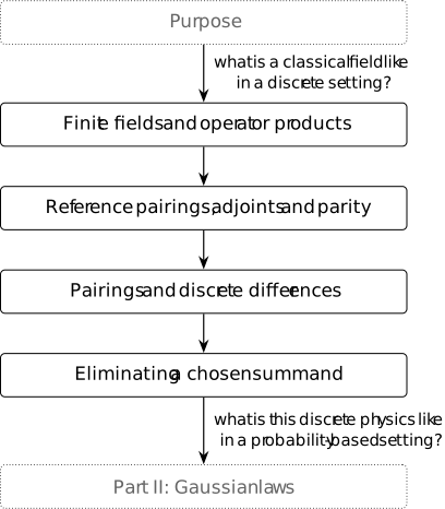
The coefficient ring is commutative and unital; the operator product need not commute. Positive counting pairings and weights enter in the real specialization. Working over a ring first separates identities of incidence, composition and elimination from positivity and integration. The general adjoint construction assumes perfect pairings, and elimination requires an invertible eliminated block; these hypotheses do not follow from the coefficient ring alone. Real positivity and measure are additional data for the later Gaussian laws.
A measurement has finite resolution, and a lattice regularisation keeps finitely many sites. Both give finite data, while the field equations are written for a continuum. Can the continuum be induced from finite data? An answer must begin with a field on finitely many points: a value at each point, or along each step between them.
Discussion 1. The field equations in three languages [fdip-00AA]AGENTDRAFTED
- November 4, 2026
Discussion 1. The field equations in three languages [fdip-00AA]AGENTDRAFTED
- November 4, 2026
In the undergraduate course on electromagnetism the field equations arrive in the language of vector calculus. With a charge density \(\rho \) and a current \(J\), and with the constants set to one, they read \[\operatorname {div} E=\rho ,\qquad \operatorname {div} B=0,\qquad \operatorname {curl} E=-\partial _t B,\qquad \operatorname {curl} B=\partial _t E+J.\] 4 equations, two vector fields, and a potential \(A\) that enters when one wants to solve them. There the potential is primitive and the fields are derived from it by a gradient, and the metric sits in the operators: the divergence, the curl and the cross product all know about lengths and angles. Every object is continuous as well: \(\rho \) is a density, and \(\partial _t\) presupposes a parameter along which to differentiate.
A course in mathematical physics rewrites the system in the language of differential forms. The potential becomes a \(1\)-form \(A\) and the field strength its exterior derivative \(F=dA\). The exterior derivative needs no metric, so \(dF=0\) is a consequence of \(d\circ d=0\) rather than an equation to impose, and gauge transformations \(A\mapsto A+d\chi \) leave \(F\) unchanged by construction, which is why gauge theory is written this way. The metric reappears in the Hodge star that the equations with sources require, \(d\star F=\star j\), while \(d\) raises the degree of a form. [hassani2013mathematical, Section 28.5] writes the field equations this way.
Readers who have met geometric calculus will recognize the same system in the unified language that Hestenes and Sobczyk proposed for mathematics and physics. The electric and magnetic fields are then grades of one object, the bivector \(F=E+IB\), where \(I\) is the pseudoscalar of the algebra, the product of the 4 frame vectors, with \(I^2=-1\), so the magnetic field enters as the dual bivector \(IB\), and the pair forms one bivector rather than the vector and pseudovector of vector calculus. The derivative is the vector derivative \(\nabla \): the derivative along each direction of a chosen frame, combined into a single vector-valued operator by the geometric product with the frame vectors. It acts by geometric multiplication, and a vector multiplied that way by a multivector splits into two parts, \[\nabla F=\nabla \cdot F+\nabla \wedge F,\] an inner product giving a divergence and an outer product giving a curl. With it the 4 equations become \(\nabla F=J\), the divergence part carrying the sources and the curl part vanishing, so each original equation returns as a definite grade. Hestenes and Sobczyk develop the calculus [hestenes2012clifford], Doran and Lasenby carry it through classical electrodynamics [doran2003geometric, Section 7.1], and Macdonald's textbook is the treatment [macdonald2012vector]. Here one algebra and one derivative serve both objects, and the metric is neither an operator nor a dual: it is inside the geometric product, which is why the language carries a chosen spacetime with it.
All three ways of writing these equations need a limit: in each, a derivative compares values at points whose separation shrinks. Those points are not bare: the continuum carries a metric, a topology and a smooth structure, and that is what gives a separation, a direction and a gradient their meaning. On a lattice only finitely many points remain, and a direction becomes a step from one site to a neighbour. What is left of the gradient is the difference of the values at the two ends of each step. A derivative of a product obeys the Leibniz rule; does a difference of values obey it as well, or does something else take its place? And which changes of the potential does a difference fail to see?
A field assigns a coefficient to each vertex or edge. Along an oriented edge, the incidence map subtracts the source value from the head value. Endpoint pullbacks express this comparison between distinct field spaces. Composition supplies an operator product on a common field module; comparing it with pointwise field multiplication gives a discrete product rule. Lemma 20 states that rule, and Example 22 shows where operator commutativity fails. The alternating four-cycle of Example 8 supplies the weights and the half-turn that the examples below use.
Definition 2. Ring-valued incidence fields [fdip-0010]AGENTDRAFTED
- October 20, 2026
Definition 2. Ring-valued incidence fields [fdip-0010]AGENTDRAFTED
- October 20, 2026
Let \(R\) be a commutative ring with identity. Choose finite sets \(V,E\) and maps \(s,h:E\to V\). The edge \(e\) goes from \(s(e)\) to \(h(e)\); loops and distinct edges with the same endpoints are allowed. Call the finite sets together with their endpoint maps the carrier. The field modules are the vertex-field module and the edge-field module \[\mathcal F_R(V)=\{f:V\to R\},\qquad \mathcal F_R(E)=\{a:E\to R\}.\] Addition, scalar multiplication and multiplication are pointwise: \[(f+g)(v)=f(v)+g(v),\quad (rf)(v)=rf(v),\quad (fg)(v)=f(v)g(v).\] These are modules and commutative unital \(R\)-algebras; the unit is the constant field \(1\).
The zero ring and an empty vertex set or edge set are allowed. On an empty set there is one field, and the constant \(1\) is also zero. No nontriviality, pairing, retained subset or positivity is assumed. The algebra convention is [stacks2017stacks, Section 22.2], Tag 09JF. The module and algebra laws are in Lemma 5.
The alternating four-cycle of Example 8 is an instance of these fields.
Definition 3. Pullbacks and the incidence map [fdip-00AQ]AGENTDRAFTED
- November 4, 2026
Definition 3. Pullbacks and the incidence map [fdip-00AQ]AGENTDRAFTED
- November 4, 2026
Let \(R\) be a commutative ring with identity, with the carrier of finite sets \(V,E\) and maps \(s,h:E\to V\), and the field modules over it. For a map \(a:E\to V\), its field pullback is \[a^*:\mathcal F_R(V)\to \mathcal F_R(E),\qquad (a^*f)(e)=f(a(e)).\] It preserves addition, scalars, products and the unit. The ring-valued incidence map is the typed difference \[d=h^*-s^*:\mathcal F_R(V)\longrightarrow \mathcal F_R(E).\] Thus \((df)(e)=f(h(e))-f(s(e))\). This is an \(R\)-linear map, with both coefficient rings equal to \(R\) and scalar homomorphism \(\sigma =\operatorname {id}_R\), as in Remark [ca-001G]. The two field modules need not coincide, so \(d^2\) has no meaning without an additional composable map. The pullback law, the linearity and the kernel of \(d\) are in Lemma 5.
For real oriented-graph incidence, see [spielman2009effective, Section 2.1, p. 4]; the ring-level claims follow from Lemma 5.
Remark 4. Incidence and the exterior derivative [fdip-00AB]AGENTDRAFTED
- November 4, 2026
Remark 4. Incidence and the exterior derivative [fdip-00AB]AGENTDRAFTED
- November 4, 2026
The potential of the preceding discussion is a field on the vertices: one value per site, added and scaled pointwise as in the vertex-field module. Along an edge the difference between the two endpoint values is what the edge carries, so the ring-valued incidence map takes a potential to the field strength read off the edges. On a cubic lattice whose steps are \(x\to x+\mu \), that difference is \(\varphi (x+\mu )-\varphi (x)\).
In the forms notation the potential is a \(0\)-form and the field strength a \(1\)-form, related by \(d\). The incidence map plays the role of \(d\) on \(0\)-forms, and it is not \(d\): the exterior derivative raises the degree of a form, while the incidence map runs from vertex fields to edge fields of one particular graph. A field pullback is composition with a map of the two finite sets, as in the substitution \(f'(x)=f(h(x))\).
Lemma 5. Basic properties of incidence fields [fdip-00AC]AGENTDRAFTED
- November 3, 2026
Lemma 5. Basic properties of incidence fields [fdip-00AC]AGENTDRAFTED
- November 3, 2026
Let \(R\) be a commutative unital ring, and let \(V,E,s,h\) and the field modules, field pullback and ring-valued incidence map be as in the two definitions above. The pointwise operations make both modules commutative unital \(R\)-algebras, the indicator fields are a basis of each, every field pullback preserves the operations, and \(d\) is \(R\)-linear. Call two vertices equivalent when they are equal or a finite sequence of edges has them as successive ends, ignoring orientation. The equivalence classes are the undirected components; a vertex that lies on no edge is a component of its own. Then \(df=0\) if and only if \(f\) is constant on each undirected component.
Proof.
- November 3, 2026
Proof.
- November 3, 2026
Every module and algebra identity follows by evaluation from the corresponding identity in \(R\). For each \(v\in V\), let \(\delta _v(u)\) be \(1\) if \(u=v\) and \(0\) otherwise. Evaluation at \(u\) proves \[f=\sum _{v\in V}f(v)\delta _v,\] and proves uniqueness of the coefficients. The same argument applies to edge fields. On an empty carrier the sum is empty and there is one field. Evaluation also proves every pullback law; for instance \(a^*(fg)(e)=f(a(e))g(a(e))\). Finally \[d(rf+g)(e)=r\bigl (f(h(e))-f(s(e))\bigr )+g(h(e))-g(s(e)),\] which proves linearity. These evaluations apply to the zero ring.
If \(df=0\), then \(f(h(e))=f(s(e))\) for every edge, so \(f\) takes the same value at the successive ends of any finite sequence of edges and is constant on each component. Conversely, the two ends of an edge lie in one component, and the two ends of a loop are the same vertex, so a field constant on each component has \(df=0\). The argument uses no division.
Remark 6. Gauge freedom of a potential [fdip-00AD]AGENTDRAFTED
- November 3, 2026
Remark 6. Gauge freedom of a potential [fdip-00AD]AGENTDRAFTED
- November 3, 2026
The kernel in Lemma 5 is the gauge freedom of the potential. Adding a constant on one undirected component leaves every edge difference unchanged, and the electric field is the negative of that difference. A vector potential is assigned to the edges, as the link variables of lattice gauge theory are, and its field strength is the difference of those values around a face. The identity \(d\circ d=0\) needs that second difference, from edge fields to face fields. The maps defined here run only from vertices to edges.
Definition 7. The incidence matrix [fdip-00AF]AGENTDRAFTED
- November 3, 2026
Definition 7. The incidence matrix [fdip-00AF]AGENTDRAFTED
- November 3, 2026
Let \(R\) be a commutative unital ring, and let \(d\) be the ring-valued incidence map of a finite carrier \(\,(V,E,s,h)\). Choose orders of the vertex and edge indicators. Let \(c_V:\mathcal F_R(V)\to R^{|V|}\) and \(c_E:\mathcal F_R(E)\to R^{|E|}\) send a field to its ordered values. The indicator expansion in Lemma 5 gives their inverses, where \(\delta _v\) is the indicator field of a vertex \(v\). The incidence matrix represents \(c_Edc_V^{-1}\): \[B_{ev}=(d\delta _v)(e)=\mathbf 1_{v=h(e)}-\mathbf 1_{v=s(e)}.\] Rows are indexed by edges and columns by vertices. A loop has a zero row; reversing an edge negates its row. This extends the oriented-graph sign convention of [spielman2009effective, Section 2.1, p. 4]. If coordinate reorderings are \(P_V,P_E\), then \(B'=P_EBP_V^{-1}\), since both sides send \(c'_V(f)\) to \(c'_E(df)\).
Example 8. The alternating four-cycle [fdip-0003]AGENTDRAFTED
- October 16, 2026
Example 8. The alternating four-cycle [fdip-0003]AGENTDRAFTED
- October 16, 2026
Let \(V=\mathbb Z/4\mathbb Z\) and \(E=\{e_0,e_1,e_2,e_3\}\), with \(s(e_i)=i\) and \(h(e_i)=i+1\) modulo \(4\). For \(t>0\), assign weights \[w_t(e_0)=w_t(e_2)=1,\qquad w_t(e_1)=w_t(e_3)=t.\] This is a weighted finite incidence presentation: the parameter \(t\) is supplied, and every edge weight is positive.
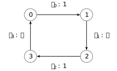
Each arrow points from source to head; the label gives its edge name and weight. A half-turn exchanges opposite vertices and edges.
On the real four-cycle, order vertices as \(0,1,2,3\) and edges as \(e_0,e_1,e_2,e_3\). The incidence matrix \(B\) of \(D\), and the coordinate array \(W_t\) of the weights, are \[B=\begin {pmatrix} -1&1&0&0\\ 0&-1&1&0\\ 0&0&-1&1\\ 1&0&0&-1 \end {pmatrix},\qquad W_t=\operatorname {diag}(1,t,1,t).\] Thus a field with ordered values \((a,b,c,d)\) has edge differences \((b-a,c-b,d-c,a-d)\). For \(f=\delta _1\), the edge values of \(Df\) are \((1,-1,0,0)\): the field rises along \(e_0\) and falls along \(e_1\).
The quadratic action of Example [fdip-002P] uses these same edge orientations and weights, with a positive mass term.
Define the half-turn on both sets by \[r_V(i)=i+2,\qquad r_E(e_i)=e_{i+2}.\] Applying either map twice adds 4, so both are involutions, and \(r_V(0)=2\) shows that the map on vertices is not the identity. Moreover, \[s(r_E(e_i))=i+2=r_V(s(e_i)),\] \[h(r_E(e_i))=i+3=r_V(h(e_i)).\] The half-turn therefore preserves the directed incidence data. Since \(i\) and \(i+2\) have the same parity, it also preserves the weights: \(w_t(r_E(e_i))=w_t(e_i)\). In contrast, a one-step rotation sends \(e_0\) to \(e_1\) and fails to preserve weights when \(t\ne 1\).
After forgetting orientations and weights, the underlying graph is
Mathlib's SimpleGraph.cycleGraph at 4 vertices, identifying
\(\operatorname {Fin}(4)\) with the residue classes modulo \(4\). That
declaration specifies the unweighted graph. The displayed matrix and
weight-preserving half-turn follow from the substitutions above.
Remark 9. Divergence and the discrete Poisson equation [fdip-00AG]AGENTDRAFTED
- November 3, 2026
Remark 9. Divergence and the discrete Poisson equation [fdip-00AG]AGENTDRAFTED
- November 3, 2026
The incidence matrix \(B\) is the difference matrix of the preceding discussion, and \(L=B^{\mathsf T}B\) is the graph Laplacian. The matrix \(-B^{\mathsf T}\) is the discrete divergence. With the edge field \(E=-B\varphi \), Gauss's law \(\nabla \cdot E=\rho \) becomes \[\,(-B^{\mathsf T})(-B\varphi )=B^{\mathsf T}B\varphi =L\varphi =\rho ,\] the discrete Poisson equation. Computations, and the later Laplacian chapters, use \(d\) in this matrix form.
Discussion 10. Products and derivatives [fdip-00AH]AGENTDRAFTED
- November 4, 2026
Discussion 10. Products and derivatives [fdip-00AH]AGENTDRAFTED
- November 4, 2026
A coupling that varies from site to site enters a lattice action as a coefficient: the term \(m\sum _v\varphi (v)^2\) for a constant mass \(m\) becomes \(\sum _v m(v)\varphi (v)^2\), so a fixed field multiplies the field at each site. Multiplying by a fixed field and taking differences along the edges are then two linear maps of one module, and composing them in the two orders gives two different maps. What is the map that multiplies, and how badly does it fail to commute with a difference?
Definition 11. Multiplication operators [fdip-00AI]AGENTDRAFTED
- November 3, 2026
Definition 11. Multiplication operators [fdip-00AI]AGENTDRAFTED
- November 3, 2026
Let \(R\) be a commutative unital ring and \(V\) a finite set. On the vertex-field module, each \(f\in \mathcal F_R(V)\) determines a multiplication operator \[M_f:\mathcal F_R(V)\to \mathcal F_R(V),\qquad M_f(g)=fg.\] The assignment \(f\mapsto M_f\) is an injective \(R\)-algebra map, \[M_{f+g}=M_f+M_g,\quad M_{rf}=rM_f,\quad M_{fg}=M_fM_g,\quad M_1=I.\] Proposition 13 proves these identities from the ring laws.
Remark 12. The potential term [fdip-00AJ]AGENTDRAFTED
- November 3, 2026
Remark 12. The potential term [fdip-00AJ]AGENTDRAFTED
- November 3, 2026
The multiplication operator \(M_V\) is the potential term of a lattice Schrödinger operator, added to a difference operator. The assignment \(f\mapsto M_f\) is how a field acts on its own module, and \(M_f M_g=M_g M_f\). A shift need not commute with \(M_f\). That product is the operator product of Proposition 13, and Example 22 computes the failure on a cycle.
Proposition 13. Composition and field multiplication [fdip-0011]AGENTDRAFTED
- October 20, 2026
Proposition 13. Composition and field multiplication [fdip-0011]AGENTDRAFTED
- October 20, 2026
Let \(R\) be a commutative unital ring. For \(R\)-modules \(M,N,P\), use \(\operatorname {Hom}_R(M,N)\) for additive, scalar-preserving maps. Thus linearity fixes \(\sigma =\operatorname {id}_R\). Given \(A\in \operatorname {Hom}_R(M,N)\) and \(B\in \operatorname {Hom}_R(N,P)\), write \[BA=B\circ A:M\to P.\] Composition is associative and \(R\)-bilinear where the types match. In particular, the endomorphisms \(\operatorname {End}_R(M)=\operatorname {Hom}_R(M,M)\) form an associative unital \(R\)-algebra, with unit \(I_M\) and central scalar map \(r\mapsto rI_M\).
On the vertex-field module, pointwise products are the multiplication operators. The map \(f\mapsto M_f\) is an injective \(R\)-algebra homomorphism into \(\operatorname {End}_R(\mathcal F_R(V))\). The proof evaluates those algebra laws. Example 22 exhibits endomorphisms that do not commute.
Proof.
- October 20, 2026
Proof.
- October 20, 2026
Pointwise addition and scalar multiplication make \(\operatorname {Hom}_R(M,N)\) a module: the linearity equations are preserved by both operations. If \(A,B\) are composable, then \(BA(rx+y)=B(rAx+Ay)=rBAx+BAy\), so \(BA\) is linear. For a third composable map \(C\), \((CB)A(x)=C(B(Ax))=C(BA)(x)\). The identity map is a two-sided unit. For composable maps with common source and target, \[\begin {aligned} B(A+A')(x)&=B(Ax)+B(A'x),\\ (B+B')A(x)&=B(Ax)+B'(Ax),\\ B(rA)(x)&=rB(Ax),\qquad (rB)A(x)=rB(Ax). \end {aligned}\] These prove distributivity and bilinearity. For an endomorphism \(A\), \((rI)A(x)=rAx=A(rx)=A(rI)(x)\), proving centrality of the scalar map; its unit, addition and product laws follow immediately by evaluation.
Pointwise multiplication makes \(M_f\) linear. Evaluating the 4 identities \[M_{f+g}=M_f+M_g,\quad M_{rf}=rM_f,\quad M_{fg}=M_fM_g,\quad M_1=I\] on a field proves them using the ring laws. If \(M_f=M_g\), applying both maps to the constant field \(1\) yields \(f=g\); this also holds when \(V\) is empty or \(R\) is the zero ring.
The Hom-module and algebra conventions are
[stacks2017stacks, Section 10.10; Section 22.2], Tags 0581 and 09JF;
the field multiplication assertions are the direct calculation above.
Mathlib's Module.End.mul_eq_comp and
Module.End.mul_apply give this right-factor-first product.
These declarations do not assert that arbitrary maps with different
endpoints form one algebra, or that a formal generator presentation is
faithful.
Lemma 14. The endpoint product identity [fdip-0012]AGENTDRAFTED
- October 20, 2026
Lemma 14. The endpoint product identity [fdip-0012]AGENTDRAFTED
- October 20, 2026
For the ring-valued incidence map \(d=h^*-s^*:\mathcal F_R(V)\to \mathcal F_R(E)\) over a commutative unital ring \(R\) and fields \(f,g\in \mathcal F_R(V)\), one has \[d(fg)=(df)(h^*g)+(s^*f)(dg).\] Every factor on the right is an edge field, and the products are pointwise in \(\mathcal F_R(E)\). Equivalently, \[d(fg)=(df)(s^*g)+(s^*f)(dg)+(df)(dg).\]
Proof.
- October 20, 2026
Proof.
- October 20, 2026
Fix an edge \(e\) and abbreviate \(f_h=f(h(e))\), \(f_s=f(s(e))\), and similarly for \(g\). Then \[\begin {aligned} (df)(e)(h^*g)(e)+(s^*f)(e)(dg)(e) &=(f_h-f_s)g_h+f_s(g_h-g_s)\\ &=f_hg_h-f_sg_s\\ &=d(fg)(e). \end {aligned}\] Equality at each edge proves the identity. Substituting \(h^*g=s^*g+dg\) gives the second formula. The proof also applies to loops, parallel edges, empty carriers and the zero ring.
This is a direct endpoint calculation. Its cyclic specialization is Lemma 20. The forward-difference convention is [wingate2025lattice, Section 4, Equations (4.2)-(4.3), p. 3]; that real-lattice convention is not an attribution of the general ring-valued incidence statement.
Discussion 15. Squares of differences [fdip-00AK]AGENTDRAFTED
- November 4, 2026
Discussion 15. Squares of differences [fdip-00AK]AGENTDRAFTED
- November 4, 2026
An action for a field on the four-cycle of Example 8 sums the squares of its differences along the edges, weighted by the edge weights \(w(e)\): that sum is the discrete form of \(\int |\nabla \varphi |^2\). A pairing sums products of the values themselves, the discrete form of \(\int fg\) when each site has unit volume. Both expressions need coefficients that can be squared and added, and a sum of squares that vanishes only when every term does. Which coefficient rings admit such a sum, and what does positivity require of the weights?
Definition 16. Finite incidence data and real fields [fdip-0002]AGENTDRAFTED
- October 16, 2026
Definition 16. Finite incidence data and real fields [fdip-0002]AGENTDRAFTED
- October 16, 2026
Specialize the field modules to \(R=\mathbb R\). The finite sets \(V,E\) and endpoint maps \(s,h:E\to V\) form a finite incidence presentation; its real specialization adds the scalar order needed for positive pairings and weights. A real vertex field is a function \(f:V\to \mathbb R\), written \(f\in \mathbb R^V\) with \(\mathbb R^V=\mathcal F_{\mathbb R}(V)\) and \(\mathbb R^E=\mathcal F_{\mathbb R}(E)\).
Their counting inner products are \[\langle f,g\rangle _V=\sum _{v\in V}f(v)g(v),\qquad \langle a,b\rangle _E=\sum _{e\in E}a(e)b(e).\] These finite sums are bilinear and symmetric. A sum of squares vanishes exactly when all its entries vanish, so they are positive definite, including on the zero space when an indexing set is empty. The real field values remain continuous even though the carrier is finite.
The real incidence map is the specialization \[D=d_{\mathbb R}:\mathbb R^V\longrightarrow \mathbb R^E,\qquad (Df)(e)=f(h(e))-f(s(e)).\] Its linearity is the specialization of the ring-valued incidence map. Loops have zero incidence, and parallel edges remain distinct. For an oriented loopless graph this is the sign convention of [spielman2009effective, Section 2.1, p. 4]; the endpoint formula extends it to loops. Connectedness and positive weights are not needed to define \(D\).
A positive edge-weight function \(w:E\to \mathbb R_{>0}\) is additional data. It acts on edge fields by \((Wa)(e)=w(e)a(e)\). Different weights change the supplied data. No retained subset belongs to this definition. The alternating four-cycle of Example 8 is one weighted instance.
For the counting inner product, Mathlib's
EuclideanSpace is the corresponding finite function space and
PiLp.inner_apply gives the sum of coordinate inner products.
These declarations concern the pairing, rather than the incidence
presentation as a whole.
Remark 17. Counting pairings and the Dirichlet sum [fdip-00AL]AGENTDRAFTED
- November 3, 2026
Remark 17. Counting pairings and the Dirichlet sum [fdip-00AL]AGENTDRAFTED
- November 3, 2026
The counting inner products are \(\int fg\) with unit volume at each site or edge. For a positive weight \(w(e)\) on each edge, \[\sum _{e\in E}w(e)\,(Df)(e)^2\] is \(\int |\nabla \varphi |^2\), and \(w(e)\) is the coupling on that edge. The Gaussian laws later in the notes need this positivity. A general commutative ring gives the difference; an order that makes a sum of squares positive is further structure.
Discussion 18. Differences on a cycle of sites [fdip-00AM]AGENTDRAFTED
- November 4, 2026
Discussion 18. Differences on a cycle of sites [fdip-00AM]AGENTDRAFTED
- November 4, 2026
Label the sites of a cycle by \(\mathbb Z/n\mathbb Z\). The difference of neighbouring values is the derivative one writes when the step has length \(1\). The product rule a difference obeys has a correction term, and on a cycle the last site is again the first: which rule holds when the shift wraps around, and what does it leave uncorrected?
Definition 19. Cyclic shift and forward difference [fdip-00AN]AGENTDRAFTED
- November 3, 2026
Definition 19. Cyclic shift and forward difference [fdip-00AN]AGENTDRAFTED
- November 3, 2026
Let \(R\) be a commutative unital ring, let \(n\ge 1\), and take \(V=\mathbb Z/n\mathbb Z\) and \(E=\{e_i:i\in V\}\), with \(s(e_i)=i\) and \(h(e_i)=i+1\). The edge-label bijection gives an \(R\)-algebra isomorphism \[j:\mathcal F_R(E)\to \mathcal F_R(V),\qquad j(a)(i)=a(e_i).\] Its inverse sends \(f\) to the edge field \(e_i\mapsto f(i)\); both preserve the pointwise operations. With the ring-valued incidence map, the cyclic shift and forward difference are \[\,(Tf)(i)=f(i+1),\qquad \Delta =jd=T-I.\] The shift is an algebra automorphism, with \(\,(T^{-1}f)(i)=f(i-1)\). Vertex and edge fields are identified only through the displayed map \(j\).
Lemma 20. A shifted product rule [fdip-0009]
L∃∀NAGENTDRAFTED
- October 16, 2026
Lemma 20. A shifted product rule [fdip-0009]
L∃∀NAGENTDRAFTED
- October 16, 2026
Let \(R\) be a commutative unital ring and let \(n\ge 1\). On \(\mathcal F_R(\mathbb Z/n\mathbb Z)\), let \(T\) and \(\Delta \) be the cyclic shift and forward difference.
For \(f,g\) in that module, \[\Delta (fg)=(\Delta f)(Tg)+f\Delta g.\] Equivalently, \[\Delta (fg)=(\Delta f)g+f\Delta g+(\Delta f)(\Delta g).\] Wingate defines forward and backward differences with lattice spacing \(a\) in [wingate2025lattice, Section 4, Equations (4.2)-(4.3), p. 3]. Here \(a=1\); the ring-valued finite identities are direct calculations, with no continuum approximation.
Proof.
- October 16, 2026
Proof.
- October 16, 2026
For every \(i\), \((jh^*f)(i)=f(i+1)=Tf(i)\) and \((js^*f)(i)=f(i)\). Applying the product-preserving map \(j\) to Lemma 14 therefore gives the first formula, where \(j\), \(s\) and \(h\) are the isomorphism and endpoint maps of that cycle. Substitute \(Tg=g+\Delta g\) to obtain the second.
At \(n=1\), the cycle has a loop and \(T=I\), \(\Delta =0\). At \(n=2\), its two edges have opposite orientations between the same vertices; it is not a single simple edge. The unshifted Leibniz rule fails by the correction \(\,(\Delta f)(\Delta g)\). On the four-cycle, \(f=\delta _1\) satisfies \(f^2=f\); at vertex \(0\), \(\,(\Delta (f^2))(0)=1\) and \(\,((\Delta f)f+f\Delta f)(0)=0\), while \(\,((\Delta f)(Tf)+f\Delta f)(0)=1\). Lemma [fdip-0014] adds a real pairing and identifies the positive kinetic factorization.
Mathlib's fwdDiff_smul proves the three-term formula for
an additive commutative monoid, a ring and a module over it. Take the
index monoid \(\mathbb Z/n\mathbb Z\), step \(1\), and the regular
\(R\)-module \(R\). Scalar multiplication is ring multiplication.
Substituting \(Tg=g+\Delta g\) yields the shifted formula; this marker
does not claim the endpoint incidence or counting-adjoint theorem.
Lemma 21. Shift and multiplication operators [fdip-0013]AGENTDRAFTED
- October 20, 2026
Lemma 21. Shift and multiplication operators [fdip-0013]AGENTDRAFTED
- October 20, 2026
Let \(R\) be a commutative unital ring and \(n\ge 1\) an integer. On \(\mathcal F_R(\mathbb Z/n\mathbb Z)\), let \(T\) and \(\Delta =T-I\) be the cyclic shift and forward difference, and let \(M_f\) be the multiplication operator of a field \(f\in \mathcal F_R(\mathbb Z/n\mathbb Z)\). As actual endomorphisms of this one module, \[TM_f=M_{Tf}T,\qquad \Delta M_f=M_{\Delta f}T+M_f\Delta .\]
Proof.
- October 20, 2026
Proof.
- October 20, 2026
For each field \(g\) and each residue class \(i\), \[(TM_fg)(i)=f(i+1)g(i+1)=(M_{Tf}Tg)(i).\] This proves the first equality. Since \(M_{\Delta f}=M_{Tf}-M_f\), \[\begin {aligned} M_{\Delta f}T+M_f\Delta &=(M_{Tf}-M_f)T+M_f(T-I)\\ &=M_{Tf}T-M_f\\ &=TM_f-M_f=\Delta M_f. \end {aligned}\] For \(n=1\), \(T=I\) and \(\Delta =0\), so the same identities hold.
The operator product is fixed in Proposition 13. For the difference convention, see [wingate2025lattice, Section 4, Equations (4.2)-(4.3), p. 3]. The proof concerns these represented maps; it asserts no universal presentation for formal generators. Example 22 is a clock and a shift for which the two products differ.
Example 22. Clock and shift [fdip-00AP]AGENTDRAFTED
- November 3, 2026
Example 22. Clock and shift [fdip-00AP]AGENTDRAFTED
- November 3, 2026
Let \(N\ge 1\) and let \(R\) be a commutative unital ring containing an element \(\omega \) with \(\omega ^N=1\). On \(\mathbb Z/N\mathbb Z\) set \(\chi (i)=\omega ^i\), let \(U=M_\chi \) be the multiplication operator of \(\chi \), and let \(T\) be the cyclic shift. Lemma 21 gives \(TU=M_{T\chi }T\). Since \(\,(T\chi )(i)=\chi (i+1)=\omega ^{i+1}=\omega \chi (i)\), one has \(M_{T\chi }=\omega U\), and therefore \(TU=\omega UT\). When \(\omega \ne 1\) the two products differ. Also \(T^N=I\) and \(U^N=M_{\chi ^N}=I\). If \(\omega \) is primitive of order \(N\), the operators \(T\), \(U\) and the powers of \(\omega \) generate a finite Heisenberg group. The four-cycle is the case \(N=4\).
The continuum form is the commutator of differentiation with multiplication by the coordinate. For a smooth function \(f\), \[\frac {d}{dx}(xf)-x\frac {d}{dx}f=f,\] so \(\bigl [\tfrac {d}{dx},x\bigr ]=1\). With \(p=-i\hbar \,d/dx\) this is \([p,x]=-i\hbar \).
The same relation holds over the field \(\mathbb F_p\) when \(N\) divides \(p-1\). Then \(X^N-1\) divides \(X^{p-1}-1=\prod _{c\in \mathbb F_p^\times }(X-c)\). The divisor is separable, because \(p\) does not divide \(N\) and \(X^N-1\) shares no root with its derivative, so it has \(N\) distinct roots in \(\mathbb F_p\). Those roots form a subgroup \(G\). Let \(m\) be the least common multiple of the orders of its elements, and factor \(m\) into prime powers. For each prime power \(q\) in that factorization, some element of \(G\) has order divisible by \(q\), and a power of it has order \(q\). The product of one such element for each prime power has order \(m\): the factors commute, and their orders are coprime. Every element of \(G\) is a root of \(X^m-1\), and a field has at most \(m\) roots of that polynomial, so \(N\le m\). Orders in \(G\) divide \(N\), so \(m\) divides \(N\). Hence \(m=N\), and \(G\) contains a primitive \(N\)-th root.