Theorem. Gauge projection and periodic-time traces [fdip-0083]
AGENTDRAFTED
For the spatial transfer data, normalized gauge
averaging is the orthogonal projection
\[\begin {aligned}
(Pf)(U)&=\int _K f(h^{-1}\cdot U)\,dh,\\
\mathcal H_{\mathrm {phys}}
&=\{f:R_hf=f\text { for every }h\in K\}=P\mathcal H_{\mathrm {link}}.
\end {aligned}\]
This defines the physical Hilbert space of neutral
states. The restriction \(T_{\mathrm {phys}}=T|_{\mathcal H_{\mathrm {phys}}}\)
is positive, injective and trace class. It is nonzero since constants
belong to \(\mathcal H_{\mathrm {phys}}\). For every integer \(N\ge 1\),
\[Z_N=\operatorname {Tr}_{\mathrm {phys}}T_{\mathrm {phys}}^N
=\operatorname {Tr}_{\mathrm {link}}(PT^N)>0.\]
The gauge projector is part of the periodic trace.
There is an explicit lattice integral for \(Z_N\). Put
\(U_N=U_0\), take independent variables
\(U_j\in X\) and \(h_j\in K\) for \(0\le j<N\), and define
\[\begin {aligned}
B_{j,e}&=U_{j,e}h_{j,s(e)}U_{j+1,e}^{-1}h_{j,t(e)}^{-1},\\
\mathcal W_N(U,h)&=
\prod _{j=0}^{N-1}e^{-V(U_j)}
\prod _{j=0}^{N-1}\prod _{e\in E_s}k(B_{j,e}).
\end {aligned}\]
Then, with normalized product Haar measures,
\[Z_N=\int _{X^N\times K^N}\mathcal W_N(U,h)\,dU\,dh.\]
Thus \(Z_N^{-1}\mathcal W_N\,dU\,dh\) is a probability law.
The temporal link \(h_{j,v}\) transports from time \(j+1\) back
to time \(j\). For \(N=1,2\), the formula retains the indexed
temporal steps; it does not identify them with edges of an ordinary
simple cycle.
For independent gauge changes \(g_j\in K\), with \(g_N=g_0\),
the transformations are
\[\begin {aligned}
U_j&\longmapsto g_j\cdot U_j,\\
h_{j,v}&\longmapsto g_{j,v}h_{j,v}g_{j+1,v}^{-1}.
\end {aligned}\]
Each \(B_{j,e}\) is conjugated by \(g_{j,t(e)}\). Therefore the
weight and measure are invariant. If \(f_j:X\to \mathbb C\)
are bounded measurable gauge-invariant functions, multiplication
by \(f_j\) preserves \(\mathcal H_{\mathrm {phys}}\), and
\[\mathbb E_N\prod _{j=0}^{N-1}f_j(U_j)
=\frac {\operatorname {Tr}_{\mathrm {phys}}
(M_{f_0}T_{\mathrm {phys}}\cdots M_{f_{N-1}}T_{\mathrm {phys}})}{Z_N}.\]
This is a finite periodic-time identity for the specified spatial
observables, with the temporal links integrated as above.
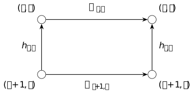
The temporal plaquette based at \((j,t)\) is traversed down
the right edge, backwards along the bottom, up the left edge and
then along the top. With the transport order, the
first transport acts on the right and the product is exactly
\(B_{j,e}\). Temporal averaging is retained at every step, so no
periodic gauge-fixing assumption removes \(P\).