Finite gauge fields and an exact torus law [fdip-006L]
✍️sourceAGENTDRAFTED
- November 1, 2026
Finite gauge fields and an exact torus law [fdip-006L]
✍️sourceAGENTDRAFTED
- November 1, 2026
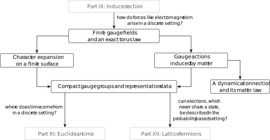
How can the transports used to compare neighboring fields themselves fluctuate? A connection background assigns a fixed transport to each edge; it is already gauge-field data. A law on those transports makes them dynamical. We now sum over them as field variables, while keeping the graph, its square faces and the group fixed. The faces are extra incidence data: the earlier graph alone does not specify them. A chosen unitary representation gives a Wilson action and a finite probability law with an explicit counting-measure convention.
Matter integration already distinguishes connections in the massive complex Gaussian on a supplied circle. Its normalized holonomy action \(W\) is minimized at trivial holonomy, so the integrated matter factor \(e^{-W}\) is largest there. That comparison leaves the circle and connection supplied. The finite law here is a further choice; transport alone does not derive a force such as electromagnetism.
Gauge averaging first determines which parts of an observable can contribute to its expectation. For the two-element group on a square torus, all plaquette signs can then be counted exactly. One global constraint and two remaining cycle holonomies account for the partition function's normalization. The resulting loop formula gives a pure-gauge area law in two dimensions; no matter field is included in that result.
Definition 1. Square faces on a finite graph [fdip-006M]AGENTDRAFTED
- November 1, 2026
Definition 1. Square faces on a finite graph [fdip-006M]AGENTDRAFTED
- November 1, 2026
A finite cubical 2-complex, in the square-cell convention used here, consists of a finite incidence presentation \((V,E,s,h)\), a finite set \(\mathcal P\) of squares, and a specified four-edge attaching walk for each square. Choose one orientation for each edge and one boundary orientation and starting vertex for each square. Its walk is \[\partial p=(e_{p,1}^{\epsilon _{p,1}},\ldots , e_{p,4}^{\epsilon _{p,4}}),\qquad \epsilon _{p,j}\in \{1,-1\},\] where an exponent \(-1\) means traversal against the chosen edge orientation. Consecutive endpoints match, including the last to the first.
Starting from the one-dimensional realization, attach one copy of \([0,1]^2\) for each \(p\), mapping its 4 sides to the specified traversed edges, and use the quotient topology. Boundary vertices or sides may be identified in this presentation, as in periodic quotients; no regularity or nonpositive-curvature condition is imposed. No higher-dimensional cubes are supplied. The squares and their attaching maps are additional data, just as the filled face is additional data in the triangle comparison.
The main example is the square torus with periods \(N_1,N_2\ge 3\). Its vertices are \[V=(\mathbb Z/N_1\mathbb Z)\times (\mathbb Z/N_2\mathbb Z).\] There are horizontal edges \(a_{x,y}:(x,y)\to (x+1,y)\) and vertical edges \(b_{x,y}:(x,y)\to (x,y+1)\), with indices read modulo the periods. The square at \((x,y)\) has boundary walk \[a_{x,y}\,b_{x+1,y}\,a_{x,y+1}^{-1}\,b_{x,y}^{-1}.\] This written order is the order of traversal. Put \[n=|V|=N_1N_2,\qquad |E|=2n,\qquad P=|\mathcal P|=n.\] The realization is the usual square grid on a torus. The periods ensure that each square has 4 distinct vertices and sides, although periodic identifications occur globally.
Definition 2. Plaquette transport and Wilson loops [fdip-006N]AGENTDRAFTED
- November 1, 2026
Definition 2. Plaquette transport and Wilson loops [fdip-006N]AGENTDRAFTED
- November 1, 2026
Let \(G\) be a finite group on a square complex. A connection is \(U\in G^E\), with \(U_{\bar e}=U_e^{-1}\) on a reversed edge. For a traversed path \(C=(e_1^{\epsilon _1},\ldots ,e_k^{\epsilon _k})\), define \[U_C=U_{e_k}^{\epsilon _k}\cdots U_{e_1}^{\epsilon _1}.\] The first transport acts on the right. The plaquette holonomy is \(U_p=U_{\partial p}\). The gauge group \(\mathcal G=G^V\) acts by \[(gU)_e=g_{h(e)}U_eg_{s(e)}^{-1}.\] Cancellation at successive vertices gives \[(gU)_C=g_{h(C)}U_Cg_{s(C)}^{-1}.\] For a closed path based at \(v\), this is conjugation by \(g_v\).
Choose a unitary representation \(\rho :G\to U(d)\) with \(d>0\), and let \(\chi _\rho (g)=\operatorname {Tr}\rho (g)\) be its character. The Wilson loop of a closed path is the unnormalized trace \[W_\rho (C)=\chi _\rho (U_C).\] It is gauge invariant. Changing the starting vertex conjugates the holonomy, so it does not change this trace. Reversing the path replaces \(U_C\) by \(U_C^{-1}\), hence replaces \(W_\rho (C)\) by its complex conjugate. In particular \(\operatorname {Re}W_\rho (C)\) is independent of the chosen boundary orientation. These are the transport and trace conventions of [wingate2025lattice, equations (6.14)–(6.19), pp. 7–8].
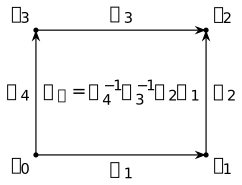
The arrows show the chosen edge orientations and the labels are connection values, not scalar weights. The boundary traversal is \[v_0\to v_1\to v_2\to v_3\to v_0.\] It uses the top and left edges backwards, accounting for both inverses.
Definition 3. The finite Wilson action and counting law [fdip-006O]AGENTDRAFTED
- November 1, 2026
Definition 3. The finite Wilson action and counting law [fdip-006O]AGENTDRAFTED
- November 1, 2026
For the finite connection data and a fixed real \(\beta \ge 0\), define the Wilson action \[S_W(U)=\beta \sum _{p\in \mathcal P} \left (1-\frac {\operatorname {Re}\chi _\rho (U_p)}d\right ).\] Since \(\rho (U_p)\) is unitary, its eigenvalues have modulus one and \(-d\le \operatorname {Re}\chi _\rho (U_p)\le d\). Thus \(S_W(U)\ge 0\). The action is gauge invariant and does not depend on starting vertices or boundary orientations.
Use unnormalized counting measure on each edge group, and therefore on \(G^E\). The partition function, probability and expectation are \[\begin {aligned} Z_W&=\sum _{U\in G^E}e^{-S_W(U)},\\ \mathbb P_W(U)&=Z_W^{-1}e^{-S_W(U)},\\ \langle F\rangle _W&=Z_W^{-1}\sum _{U\in G^E}F(U)e^{-S_W(U)}. \end {aligned}\] These finite sums have \(0<Z_W<\infty \). Matrix-valued observables are averaged entry by entry. The finite group and chosen representation are inputs to this law, alongside the square complex and \(\beta \).
The constant term in the action matters for the partition function. With \(P=|\mathcal P|\), put \[\begin {aligned} \mathcal Z(\beta ) &=\sum _{U\in G^E}\exp \left ( \frac \beta d\sum _p\operatorname {Re}\chi _\rho (U_p)\right ),\\ Z_W(\beta )&=e^{-\beta P}\mathcal Z(\beta ). \end {aligned}\] The two weights define the same normalized expectation. Replacing each edge's counting measure by uniform probability measure instead gives \(|G|^{-|E|}Z_W\); that is a different partition-function normalization, again with the same expectation. In particular \(Z_W(0)=|G|^{|E|}\). The action and expectation agree with the conventions in [wingate2025lattice, equations (6.20)–(6.21), p. 8]; that source uses normalized Haar integration for its compact-group setting, whereas the finite counting convention here is explicit.
Theorem 4. Finite gauge averaging [fdip-006P]AGENTDRAFTED
- November 1, 2026
Theorem 4. Finite gauge averaging [fdip-006P]AGENTDRAFTED
- November 1, 2026
For the finite Wilson law, define \[(\mathcal AF)(U)=\frac 1{|\mathcal G|} \sum _{g\in \mathcal G}F(gU),\qquad \mathcal G=G^V.\] Then \(\mathcal A\) projects onto gauge-invariant observables and \[\langle F\rangle _W=\langle \mathcal AF\rangle _W.\] In particular \(\langle F\rangle _W=0\) whenever \(\mathcal AF=0\). A general noninvariant observable may have a nonzero invariant part; only \(F-\mathcal AF\) is always forced to have zero expectation.
Proof.
- November 1, 2026
Proof.
- November 1, 2026
For each \(g\), the map \(U\mapsto gU\) is a bijection of \(G^E\) with inverse \(U\mapsto g^{-1}U\). Gauge invariance of the action and change of variable in a finite sum give \[\sum _U F(gU)e^{-S_W(U)}=\sum _U F(U)e^{-S_W(U)}.\] Divide by \(Z_W\) and average over \(g\). Reindexing \(g\mapsto gh\) gives \((\mathcal AF)(hU)=(\mathcal AF)(U)\). If \(F\) is already invariant then \(\mathcal AF=F\), proving \(\mathcal A^2=\mathcal A\) and the asserted range.
Let \(\sigma \) be a nontrivial irreducible complex representation of \(G\), and let \(e\) have distinct endpoints. Then \[\langle \sigma (U_e)\rangle _W=0.\] To see this, set \(R=|G|^{-1}\sum _{a\in G}\sigma (a)\). Reindexing shows that \(\sigma (b)R=R\) for every \(b\), so \(R\) maps into the fixed-vector space. It is the identity on that space. A nonzero fixed vector would span a trivial subrepresentation; irreducibility and nontriviality therefore make the fixed-vector space zero and \(R=0\). Averaging the gauge transformation at \(h(e)\) while fixing the other vertices now replaces \(\sigma (U_e)\) by \(R\sigma (U_e)=0\). The expectation is unchanged by this averaging, by the same finite change-of-variable proof. Distinct endpoints are essential here.
For a self-loop, the transformation is only conjugation. The one-loop example shows that its expectation need not vanish.
This is a direct finite averaging proof, related to
Maschke averaging. Mathlib's
Representation.isProj_averageMap proves projection onto
invariants for a finite group representation over a commutative ring
in which the group order is invertible. Over \(\mathbb C\), apply it
to the inverse-pullback representation
\((R_gF)(U)=F(g^{-1}U)\), or to \(\sigma \) above. This supports the
linear averaging step, not the Wilson probability or torus formulas.
Example 5. A self-loop with nonzero expectation [fdip-006T]AGENTDRAFTED
- November 1, 2026
Example 5. A self-loop with nonzero expectation [fdip-006T]AGENTDRAFTED
- November 1, 2026
For a self-loop \(e\), the transformation is only conjugation. In the square-cell convention, take one vertex, one loop and one square whose attaching walk traverses that loop 4 times. Use the finite Wilson law. With \(G=\{1,\omega ,\omega ^2\}\) and \(\omega =e^{2\pi i/3}\), use the one-dimensional representation \(\rho (U)=U\). Then \(U_p=U^4=U\), the gauge action is trivial, and \[\langle U\rangle _W =\frac {1-e^{-3\beta/2}}{1+2e^{-3\beta/2}}>0\qquad (\beta >0).\] Thus no general open-edge vanishing conclusion extends to self-loops.
Lemma 6. Plaquette signs and the two torus holonomies [fdip-006Q]AGENTDRAFTED
- November 1, 2026
Lemma 6. Plaquette signs and the two torus holonomies [fdip-006Q]AGENTDRAFTED
- November 1, 2026
On the square torus, let \(G=\mathbb Z_2=\{1,-1\}\) under multiplication, with \(n=|V|=P\) and \(|E|=2n\). The map sending a connection to its plaquette signs has image exactly \[\left \{(u_p)\in \{1,-1\}^{\mathcal P}:\prod _pu_p=1\right \}.\] Every such sign configuration has \(2^{n+1}\) preimages in \(G^E\). It consists of 4 gauge orbits, distinguished by two fundamental cycle holonomies.
Proof.
- November 1, 2026
Proof.
- November 1, 2026
Each edge occurs twice among the square boundaries, so \(\prod _pU_p=1\). Conversely, choose a spanning tree in the connected dual graph, whose vertices are squares and whose edges cross their shared primal edges. Root this tree and set all primal edge signs to \(1\). Process dual leaves towards the root. At each leaf, its unique remaining dual-tree edge crosses a primal edge shared with its parent. Flip that primal sign exactly when needed to give the leaf its prescribed plaquette sign, then remove the leaf. This changes only the leaf and its parent among the unprocessed squares and changes no previously fixed square. At the last square, the global product constraint forces the prescribed root sign. This constructs every even-parity plaquette pattern.
The plaquette map is a homomorphism between finite abelian groups. Multiplication by one preimage identifies its kernel with any nonempty fiber. There are \(2^{P-1}\) target patterns, hence each fiber has \[\frac {2^{|E|}}{2^{P-1}}=2^{n+1}\] elements. For a connected graph, a gauge transformation fixes an abelian connection exactly when \(g_{h(e)}=g_{s(e)}\) on every edge, that is, when all vertex values are the same. The stabilizer has two elements, so every gauge orbit has \(2^{n-1}\) elements. The fiber therefore contains \(2^{n+1}/2^{n-1}=4\) orbits.
Take a horizontal fundamental cycle in one row and a vertical one in one column. Multiply by \(-1\) every horizontal edge crossing the periodic seam from \(x=N_1-1\) to \(x=0\). Each plaquette contains zero or two such edges, so its sign is unchanged, while the horizontal cycle holonomy flips and the vertical one does not. The analogous vertical seam operation flips just the other holonomy. The two operations give 4 possibilities for these gauge-invariant signs. They are distinct gauge orbits, and the count above shows that they exhaust the 4 orbits in each plaquette fiber.
Theorem 7. The exact pure-gauge torus law [fdip-006R]AGENTDRAFTED
- November 1, 2026
Theorem 7. The exact pure-gauge torus law [fdip-006R]AGENTDRAFTED
- November 1, 2026
For the square torus, take \(G=\{1,-1\}\) in its one-dimensional sign representation and use the counting convention. With \(n=|V|=P\) and \(\beta \ge 0\), \[\begin {aligned} \mathcal Z(\beta ) &=2^{n+1}\,\frac {(2\cosh \beta )^P+(2\sinh \beta )^P}{2},\\ Z_W(\beta )&=e^{-\beta P}\mathcal Z(\beta ). \end {aligned}\] Let \(C\) be a simple contractible edge loop bounding a specified disk of \(A\) square faces, where \(0<A<P\). Put \(t=\tanh \beta \). Its Wilson loop is \(W(C)=U_C\in \{1,-1\}\), and \[\langle W(C)\rangle _W =\frac {t^A+t^{P-A}}{1+t^P}.\] The finite formula includes the complementary region through the second term.
Proof.
- November 1, 2026
Proof.
- November 1, 2026
Write \(u_p=U_p\). By the plaquette counting lemma, every pattern with \(\prod _pu_p=1\) has \(2^{n+1}\) preimages. The indicator of this constraint is \((1+\prod _pu_p)/2\). Therefore \[\begin {aligned} \mathcal Z(\beta ) &=\frac {2^{n+1}}2\sum _{u\in \{1,-1\}^{\mathcal P}} \left (1+\prod _pu_p\right )\prod _p e^{\beta u_p}\\ &=\frac {2^{n+1}}2 \left [(2\cosh \beta )^P+(2\sinh \beta )^P\right ]. \end {aligned}\] Here each unweighted one-sign sum is \(2\cosh \beta \) and each sign-weighted sum is \(2\sinh \beta \). The displayed Wilson action constant gives the formula for \(Z_W\).
Multiplying the plaquette signs inside the chosen disk cancels every interior edge twice and leaves exactly the boundary product, so \(W(C)=\prod _{p\text { inside }C}u_p\). Insert this product into the preceding constrained sum. The two terms in the unnormalized numerator, after removing the common factor \(2^{n+1}/2\), are \[\begin {aligned} &(2\sinh \beta )^A(2\cosh \beta )^{P-A},\\ &(2\cosh \beta )^A(2\sinh \beta )^{P-A}. \end {aligned}\] Divide by the corresponding partition function and then by \((2\cosh \beta )^P\). The common action constant cancels, proving the expectation formula.
Fix \(\beta >0\) and a finite disk loop while both torus periods grow, so \(A\) stays fixed and \(P\to \infty \). Then \(0<t<1\), giving \[\begin {aligned} \lim _{P\to \infty }\langle W(C)\rangle _W &=t^A=e^{-\sigma A},\\ \sigma &=-\log (\tanh \beta )>0. \end {aligned}\] This is an exact area law for this two-dimensional pure-gauge limit. It is not a claim for a matter-coupled law or for higher-dimensional lattices. At \(\beta =0\), the finite formula instead gives zero for these nonempty proper disk loops, and \(Z_W(0)=2^{2n}\).
Example 8. A three-by-three torus calculation [fdip-006S]AGENTDRAFTED
- November 1, 2026
Example 8. A three-by-three torus calculation [fdip-006S]AGENTDRAFTED
- November 1, 2026
For \(N_1=N_2=3\), there are 9 vertices, 18 edges and 9 plaquettes. The plaquette constraint permits only an even number \(k\) of negative plaquettes. There are \(\binom 9k\) such patterns and \(2^{10}=1024\) edge configurations for each pattern. The resulting numbers of edge configurations are \[\begin {array}{c|rrrrr} k&0&2&4&6&8\\\hline \text {count}&1024&36864&129024&86016&9216. \end {array}\] They sum to \(262144=2^{18}\), the number of all edge assignments.
Since \(\sum _pU_p=9-2k\), the partition polynomial is \[\begin {aligned} \mathcal Z(\beta )=1024\bigl (&e^{9\beta }+36e^{5\beta }+126e^\beta \\ &+84e^{-3\beta }+9e^{-7\beta }\bigr ),\\ Z_W(\beta )&=e^{-9\beta }\mathcal Z(\beta ). \end {aligned}\] At \(\beta =0\), this again gives \(2^{18}\). The factor \(e^{-9\beta }\) is necessary for the Wilson-action partition function even though it cancels from every normalized observable.
For \(\tanh \beta =1/2\), the exact loop formula gives \[\begin {aligned} \langle W(C_1)\rangle _W &=\frac {(1/2)+(1/2)^8}{1+(1/2)^9}=\frac {86}{171},\\ \langle W(C_2)\rangle _W &=\frac {(1/2)^2+(1/2)^7}{1+(1/2)^9}=\frac {44}{171}. \end {aligned}\] Here \(C_1\) bounds one square and \(C_2\) bounds two adjacent squares, each a simple disk boundary on this torus. These values include the finite-volume corrections; they are not yet \(t\) and \(t^2\).