Local Gaussian laws and gluing [fdip-0063]
✍️sourceAGENTDRAFTED
- November 1, 2026
Local Gaussian laws and gluing [fdip-0063]
✍️sourceAGENTDRAFTED
- November 1, 2026
Eliminating fields gives a law on a subset of vertices. This chapter asks the reverse question: when do prescribed laws on overlapping subsets come from one global law? Agreement on overlaps is necessary, but it can leave many extensions or permit none. The distinction is already visible on two vertices and on a four-cycle.
Zeros in a positive precision matrix express conditional independence. They give an exact density formula for joining two laws across a separator. For a chordal graph, its maximal cliques can be arranged in a junction tree, so the formula can be iterated. The resulting law is unique with the stated Markov condition. This finite gluing result is distinct from scalar factorization and from a stack of background objects.
Definition 1. Local Gaussian data and marginal restriction [fdip-0064]AGENTDRAFTED
- November 1, 2026
Definition 1. Local Gaussian data and marginal restriction [fdip-0064]AGENTDRAFTED
- November 1, 2026
Fix a finite vertex set \(V\). For every subset \(T\subseteq V\), let \(\mathcal G(T)\) be the set of centered real Gaussian probability laws on \(\mathbb R^T\) with positive-definite covariance. Put \(\mathcal G(\varnothing )=\{1\}\), the unit mass on the zero-dimensional space. For \(S\subseteq T\), coordinate projection \(\pi _{S,T}:\mathbb R^T\to \mathbb R^S\) defines marginal restriction \[\operatorname {res}_{S,T}\mu =(\pi _{S,T})_*\mu .\] If \(\mu =N(0,G)\), its restriction is \(N(0,G_{SS})\); a principal submatrix of \(G>0\) is positive definite. Identity and composition of projections make \(\mathcal G\) a presheaf on the poset of all subsets of \(V\).
A cover of \(T\) is a finite family \((T_i)\) with \(\bigcup _iT_i=T\). A family \(\mu _i\in \mathcal G(T_i)\) is compatible local Gaussian data if its two marginals on each \(T_i\cap T_j\) agree. A global extension is a law \(\mu \in \mathcal G(T)\) with these restrictions. In covariance coordinates, compatibility means equality of the two principal submatrices on each overlap.
The domain contains all subsets and all such positive Gaussian laws. It is not restricted to the Markov laws of one fixed graph: marginalizing vertices can create new precision entries. For a law with precision \(Q=G^{-1}\), the Schur formula gives the precision of its \(S\)-marginal as \[\Lambda _S=(G_{SS})^{-1} =Q_{SS}-Q_{S,S^c}Q_{S^c,S^c}^{-1}Q_{S^c,S},\] where \(S^c=T\setminus S\). This is generally different from \(Q_{SS}\). Empty blocks follow the zero-dimensional convention.
The two-singleton example shows why overlap compatibility alone does not ensure uniqueness.
Example 2. One-vertex marginals with many extensions [fdip-006A]AGENTDRAFTED
- November 1, 2026
Example 2. One-vertex marginals with many extensions [fdip-006A]AGENTDRAFTED
- November 1, 2026
Compatibility of local Gaussian data alone does not imply uniqueness. On the cover \(\{0\},\{1\}\) of two vertices, prescribe a standard normal law at each vertex. Every covariance \[G_\rho =\begin {pmatrix}1&\rho \\\rho &1\end {pmatrix}, \qquad -1<\rho <1,\] is a positive-definite global extension. The product law is the member \(\rho =0\). Uniqueness will require an additional conditional-independence condition.
Theorem 3. Precision zeros and Gaussian conditional independence [fdip-0065]AGENTDRAFTED
- November 1, 2026
Theorem 3. Precision zeros and Gaussian conditional independence [fdip-0065]AGENTDRAFTED
- November 1, 2026
Let \(\phi \sim N(0,Q^{-1})\) on \(\mathbb R^V\), where \(Q\) is any real symmetric positive-definite matrix. Its precision graph has an edge \(\{a,b\}\) for distinct vertices exactly when \(Q_{ab}\ne 0\). For pairwise disjoint subsets \(A,B,S\), say that \(S\) separates \(A\) from \(B\) if every graph path from \(A\) to \(B\) meets \(S\). Then \[S\text { separates }A\text { from }B \quad \Longrightarrow \quad \phi _A\mathrel {\perp \mkern -9mu\perp }\phi _B\mid \phi _S.\] Here conditional independence means that the conditional joint law factors into its two conditional marginals almost everywhere in \(\phi _S\). The canonical Gaussian density kernels used below factor at every conditioning value. For distinct vertices there is also the pairwise equivalence \[Q_{ab}=0\quad \Longleftrightarrow \quad \phi _a\mathrel {\perp \mkern -9mu\perp }\phi _b \mid \phi _{V\setminus \{a,b\}}.\] No Laplacian sign condition on \(Q\) is required.
Proof.
- November 1, 2026
Proof.
- November 1, 2026
First suppose \(V=A\sqcup S\sqcup B\). Separation implies \(Q_{AB}=0\). With \(\phi _S=s\) fixed, the quadratic energy in \(a,b\) is the sum \[\begin {aligned} &\frac 12a^TQ_{AA}a+a^TQ_{AS}s\\ &\qquad +\frac 12b^TQ_{BB}b+b^TQ_{BS}s +\frac 12s^TQ_{SS}s. \end {aligned}\] The last term is constant. The two remaining positive Gaussian factors normalize separately, proving independence at every \(s\). Equivalently, the conditional precision is \(\operatorname {diag}(Q_{AA},Q_{BB})\); its inverse has zero cross block. The square completion is the coordinate case of Proposition [fdip-0060].
For smaller disjoint \(A,B,S\), no connected component of the graph on \(V\setminus S\) meets both \(A\) and \(B\). Assign its components to two unions \(A',B'\) with \(A\subseteq A'\), \(B\subseteq B'\) and \(A'\sqcup B'=V\setminus S\); components meeting neither may be assigned arbitrarily. The preceding argument gives conditional independence of \(\phi _{A'}\) and \(\phi _{B'}\) given \(s\). Taking coordinate marginals gives the asserted independence of \(\phi _A\) and \(\phi _B\).
For the pairwise statement, fixing all other coordinates leaves conditional precision and cross covariance \[\begin {pmatrix}Q_{aa}&Q_{ab}\\Q_{ab}&Q_{bb}\end {pmatrix}, \qquad \operatorname {Cov}(\phi _a,\phi _b\mid \phi _{V\setminus \{a,b\}}) =\frac {-Q_{ab}}{Q_{aa}Q_{bb}-Q_{ab}^2}.\] The denominator is positive. Independence implies zero covariance, and zero \(Q_{ab}\) makes the conditional density a product. This proves both directions.
A positive Gaussian law is Markov with respect to a graph \(\Gamma \) if its precision is zero on all distinct nonedges of \(\Gamma \); extra zeros on edges are allowed. The same proof gives conditional independence across every separator of \(\Gamma \). Conversely its separator condition implies these zeros by taking \(S=V\setminus \{a,b\}\) for each nonedge. This is the finite Gaussian global Markov equivalence of [speed1986gaussian, Proposition 1 and Corollary 1, p. 139; Proposition 2, pp. 140–141]. The lattice harmonic-field statements of [friedli2017statistical, Theorems 8.17 and 8.26, pp. 391 and 399] concern their specified lattice precisions, not this arbitrary-precision theorem.
Mathlib's
ProbabilityTheory.HasGaussianLaw.indepFun_of_covariance_eval
supports the independence step for two finite coordinate families
with a jointly Gaussian law and zero cross covariances. Apply it
separately to the conditional Gaussian at each fixed \(s\); the block
inverse above verifies its covariance hypothesis. The declaration
asserts ordinary independence under that probability law. Graph
separation, the passage to conditional kernels and the pairwise
converse are supplied by the argument above.
Theorem 4. Gluing two Gaussian laws across a separator [fdip-0066]AGENTDRAFTED
- November 1, 2026
Theorem 4. Gluing two Gaussian laws across a separator [fdip-0066]AGENTDRAFTED
- November 1, 2026
Let \(V=V_1\cup V_2\), \(S=V_1\cap V_2\), \(A=V_1\setminus S\) and \(B=V_2\setminus S\). Suppose positive-definite centered Gaussian laws \(\mu _1,\mu _2\) have the same marginal \(\mu _S\). Write \(p_1,p_2,p_S\) for their positive Lebesgue densities. There is exactly one positive Gaussian extension with \(\phi _A\mathrel {\perp \mkern -9mu\perp }\phi _B\mid \phi _S\). Its density is \[p(a,s,b)=\frac {p_1(a,s)p_2(s,b)}{p_S(s)}.\] If \(S=\varnothing \), take \(p_S=1\); this is the product law.
Let \(\Lambda _1,\Lambda _2,\Lambda _S\) denote the three marginal precision matrices. Padding a matrix on \(T\) with zeros gives the matrix on \(V\) defined by \[\operatorname {pad}_T(M)=\pi _T^TM\pi _T.\] The extension's precision is \[Q=\operatorname {pad}_{V_1}(\Lambda _1) +\operatorname {pad}_{V_2}(\Lambda _2) -\operatorname {pad}_S(\Lambda _S).\] In particular, if a positive global Gaussian law has \(S\) separating \(A\) and \(B\) in its precision graph, this formula reconstructs its precision from the indicated marginals. The matrices \(\Lambda _i\) are marginal precisions, not principal restrictions of \(Q\).
Proof.
- November 1, 2026
Proof.
- November 1, 2026
Factor the proposed density as \(p_S(s)p_1(a\mid s)p_2(b\mid s)\). Successively integrating over \(a,b,s\) gives total mass one. Integrating just \(b\) or just \(a\) recovers \(p_1\) or \(p_2\), respectively; its conditional density is visibly a product. Completing the two local squares writes the quadratic form in its exponent \(-q/2\) as \[\begin {aligned} q(a,s,b)={}&s^T\Lambda _Ss +(a-M_1s)^TD_1(a-M_1s)\\ &+(b-M_2s)^TD_2(b-M_2s), \end {aligned}\] where \(D_1,D_2>0\) are the conditional precisions and \(M_1,M_2\) are the conditional mean maps. This form is positive definite: if it is zero, its three nonnegative terms force first \(s=0\), then \(a=b=0\). The density is therefore a centered positive Gaussian. Subtracting the three density exponents gives the displayed padding formula. These statements include empty coordinate spaces.
For any extension with the asserted conditional independence, its conditional marginals must equal the two prescribed conditional marginals almost everywhere. Its density is consequently the same product almost everywhere, proving uniqueness as a probability law. For an existing global law the Markov theorem supplies this independence. This is the density factorization underlying [speed1986gaussian, Propositions 1–2, pp. 139–141]; the construction here also proves positive-definite existence from the two compatible input laws.
The four-cycle calculation displays the marginal precisions and reconstructs every entry by this formula.
Example 5. Separator reconstruction on the four-cycle [fdip-006B]AGENTDRAFTED
- November 1, 2026
Example 5. Separator reconstruction on the four-cycle [fdip-006B]AGENTDRAFTED
- November 1, 2026
Apply separator gluing to the unit four-cycle with mass \(m=1\).
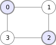
The doubled vertices form the separator \(S=\{0,2\}\). The cover sets are \(V_1=\{0,1,2\}\) and \(V_2=\{0,2,3\}\); their private vertices \(1,3\) have no connecting edge. The graph has only the 4 drawn edges, with no diagonal edge. Its precision is \[Q=\begin {pmatrix} 3&-1&0&-1\\-1&3&-1&0\\0&-1&3&-1\\-1&0&-1&3 \end {pmatrix}.\] Use \(V_1=(0,1,2)\), \(V_2=(0,2,3)\) and \(S=(0,2)\), with the listed coordinate orders. Each omitted vertex has precision \(3\), so the Schur formula gives \[\begin {aligned} \Lambda _1&=\begin {pmatrix} 8/3&-1&-1/3\\-1&3&-1\\-1/3&-1&8/3 \end {pmatrix},\\ \Lambda _2&=\begin {pmatrix} 8/3&-1/3&-1\\-1/3&8/3&-1\\-1&-1&3 \end {pmatrix},\\ \Lambda _S&=\begin {pmatrix}7/3&-2/3\\-2/3&7/3\end {pmatrix}. \end {aligned}\] Both triple laws have this same overlap marginal. Padding and subtracting gives \(Q\) entry by entry: each overlap diagonal is \(8/3+8/3-7/3=3\), and the induced overlap entry is \(-1/3-1/3+2/3=0\). The remaining edges retain weight \(-1\). The determinants are \(15,15,5\), respectively, so the glued normalization gives \(\det Q=15\cdot15/5=45\), agreeing with its eigenvalues \(1,3,3,5\). This uses one separator of a non-chordal cycle; it does not assert that arbitrary edge laws on that cycle glue.
Example 6. Compatible edge laws with no global extension [fdip-0067]AGENTDRAFTED
- November 1, 2026
Example 6. Compatible edge laws with no global extension [fdip-0067]AGENTDRAFTED
- November 1, 2026
On the four-cycle \(0,1,2,3,0\), prescribe centered Gaussian edge laws with unit variances and correlations \[\rho _{01}=\rho _{12}=\rho _{23}=\frac 9{10}, \qquad \rho _{30}=-\frac 9{10}.\] Each edge covariance has eigenvalues \(1/10,19/10\), hence is positive definite. All overlap singleton laws are \(N(0,1)\). Nevertheless there is no global positive-semidefinite covariance matrix with these entries, and therefore no global Gaussian extension.
Proof.
- November 1, 2026
Proof.
- November 1, 2026
In any joint law with these second moments, \[\|\phi _0-\phi _3\|_{L^2}=\sqrt {19/5}, \qquad \|\phi _i-\phi _{i+1}\|_{L^2}=\sqrt {1/5} \quad (i=0,1,2).\] But the first difference is the sum of the three consecutive differences. The triangle inequality would give \(\sqrt {19/5}\le 3\sqrt {1/5}\), contradicting \(19>9\). Any proposed positive-semidefinite covariance is a Gram matrix of real vectors and obeys the same norm inequality. Thus the obstruction already rules out semidefinite completion, without a nondegeneracy assumption.
The angular description gives another view of the same obstruction. Unit Gram vectors have consecutive angles \(\alpha =\arccos (9/10)\) and endpoint angle \(\pi -\alpha \). For unit vectors with successive angles \(\beta ,\gamma \) and \(\beta +\gamma \le \pi \), orthogonal decomposition along the middle vector and Cauchy–Schwarz give \[\langle u,w\rangle \ge \cos \beta \cos \gamma -\sin \beta \sin \gamma =\cos (\beta +\gamma ).\] Since arccosine decreases, the endpoint angle is at most \(\beta +\gamma \). If the sum exceeds \(\pi \), that bound is automatic. Iteration gives endpoint angle at most \(3\alpha \). But \(\alpha <\pi/4\), because \(9/10>1/\sqrt 2\); hence \(3\alpha <\pi -\alpha \), again a contradiction.
This example concerns the presheaf of laws on the edge cover: agreement on every overlap does not ensure existence. It is a concrete non-chordal obstruction of the kind distinguished by [grone1984positive, Theorem 7, p. 120]. It does not say that all data on a non-chordal graph fail to extend; the global four-cycle law in Example 5 supplies data that do extend.
Theorem 7. Chordal Gaussian gluing along a junction tree [fdip-0068]AGENTDRAFTED
- November 1, 2026
Theorem 7. Chordal Gaussian gluing along a junction tree [fdip-0068]AGENTDRAFTED
- November 1, 2026
A clique is a vertex subset whose distinct vertices are pairwise adjacent; a maximal clique is inclusion-maximal. A finite simple graph \(\Gamma \) on \(V\) is chordal if it has no induced cycle of length at least 4. Suppose centered positive-definite Gaussian laws \(\mu _K\) on its maximal cliques agree on every overlap. Then there is a unique centered positive-definite Gaussian law with these clique marginals that is Markov with respect to \(\Gamma \). Uniqueness is asserted within that Markov class.
The maximal cliques admit a junction tree: a tree \(\mathcal T\) whose nodes are the maximal cliques, such that the nodes containing any given vertex form a connected subtree. This is the running-intersection property. Write \(S_e=K\cap K'\) for the separator on an edge \(e=KK'\) and \(p_{S_e}\) for its common marginal density. Empty separators have density one. The glued law and precision are \[p(\phi )=\frac {\prod _Kp_K(\phi _K)} {\prod _{e\in E(\mathcal T)}p_{S_e}(\phi _{S_e})},\] \[Q=\sum _K\operatorname {pad}_K(\Lambda _K) -\sum _{e\in E(\mathcal T)} \operatorname {pad}_{S_e}(\Lambda _{S_e}).\] Separator terms are counted once per tree edge, including repetitions of the same vertex subset. For \(V=\varnothing \) the law is the unit mass and both products are empty.
Proof.
- November 1, 2026
Proof.
- November 1, 2026
We first justify the finite junction-tree construction. A vertex is simplicial when its neighbors form a clique. Every noncomplete chordal graph has two nonadjacent simplicial vertices. Here is an induction proof. In the connected case choose nonadjacent vertices \(a,b\) and an inclusion-minimal separator \(S\). Let \(C_a,C_b\) be their components in \(\Gamma \setminus S\). Minimality implies that each \(s\in S\) has a neighbor in both components: otherwise restoring that \(s\) would still leave \(a,b\) separated. If nonadjacent \(x,y\) belonged to \(S\), choose shortest \(x\)-to-\(y\) paths with internal vertices in \(C_a\) and in \(C_b\). Each path has no chord, and there are no edges between their interiors. Their union would be an induced cycle of length at least 4. Thus \(S\) is a clique.
Each induced graph \(C_a\cup S\) and \(C_b\cup S\) is smaller and chordal. If one is complete, any vertex in its component is simplicial. Otherwise induction gives two nonadjacent simplicial vertices; at most one lies in the clique \(S\), so choose one outside \(S\). Its full-graph neighbors still lie in that same induced graph, so it is simplicial in \(\Gamma \). The two choices are nonadjacent. In a disconnected graph choose a simplicial vertex in each of two components by the same induction; complete components pose no problem. Complete graphs have every vertex simplicial. This proves the assertion and allows repeated deletion of a simplicial vertex, a perfect elimination order.
Induct on that deletion to construct the clique tree. Remove a simplicial vertex \(v\), and write \(N\) for its neighbor clique. Unless no vertices remain, \(N\) lies in a maximal clique \(C\) of the remaining graph; when \(N=\varnothing \), choose any such \(C\). If \(N=C\), replace node \(C\) in its clique tree by \(C\cup \{v\}\). If \(N\subsetneq C\), attach \(N\cup \{v\}\) as a new leaf at \(C\). These are precisely the changes to the maximal cliques. In either case the nodes containing each old vertex remain connected, while \(v\) occurs only in the new node. A one-vertex graph starts the induction. Connecting different graph components in this way uses empty separators. This proves the required running-intersection property. The perfect-elimination characterization is also stated in [grone1984positive, Theorem 6, p. 119].
Now remove a leaf clique \(K\) of \(\mathcal T\) with neighbor \(C\) and separator \(S=K\cap C\). Running intersection says that \(A=K\setminus S\) occurs in no other clique, and that \(K\)'s intersection with the union of the remaining cliques is exactly \(S\). By induction glue the remaining clique laws; a one-clique tree starts with its prescribed law. The remaining law's marginal on \(S\) is the prescribed one, since it has the prescribed law on \(C\). The two-law theorem then glues in \(\mu _K\) by multiplication by \(p_K/p_S\). This proves normalization, positive definiteness, all clique marginals and the density formula. The precision formula follows at each step. Every nonzero summand is supported on a clique, so the precision is zero on all nonedges: the constructed law is Markov.
For uniqueness, \(S\) separates \(A\) from the remaining vertices outside \(S\): an edge out of \(A\) would belong to a maximal clique, but no other clique contains its endpoint in \(A\). Any Markov extension therefore factors across this separator by Theorem 3. Its marginal after removing \(A\) is again Markov for the induced remaining graph. Indeed the Schur correction from eliminating \(A\) is supported only on \(S\times S\), and \(S\) is a clique, so it creates no entry on a nonedge. Induction makes that remaining marginal unique; the separator factorization then makes the full law unique.
The positive-definite completion theorem of [grone1984positive, Theorem 7, p. 120, proof pp. 121–122] characterizes chordal graphs by existence for every compatible positive clique specification. The proof above additionally constructs the Markov extension and proves uniqueness within that class. Bare completion existence alone does not assert that all extensions are identical. Even for two isolated vertices, Example 2 has many positive completions and exactly one Markov completion.
Remark 8. What the gluing theorem establishes about descent [fdip-0069]AGENTDRAFTED
- November 1, 2026
Remark 8. What the gluing theorem establishes about descent [fdip-0069]AGENTDRAFTED
- November 1, 2026
The presheaf of Gaussian laws has an explicit domain, restriction maps and overlap compatibility. On the finite-subset poset with covers given by unions, it is not a sheaf: the two-singleton cover has non-unique extensions, and the four-cycle edge cover has compatible data with no extension. These are separate failures of uniqueness and existence.
The chordal theorem gives a precise replacement on a specified clique cover. It chooses the unique extension satisfying that graph's Markov condition and supplies its density and precision. A different graph or a different collection of local laws is a different problem. This does not turn fixed-graph Markov laws into a presheaf closed under every marginal restriction; Schur elimination can introduce precision edges.
The earlier factorization comparison separates scalar factorization, functorial factorization, localization and descent. The present result adds a concrete finite local-to-global theorem for laws, but no descent data for the objects and arrows of the background groupoid. A stack would require a specified site, a category fibred over it, sheaves of morphisms and effective object descent [stacks2017stacks, Definition 8.4.1], Tag 0268. No such stack assertion follows from the density gluing formula; stack-level gluing of background objects remains an additional question.