Gauss's law and charged multiplicities [fdip-0088]
✍️sourceAGENTDRAFTED
- November 1, 2026
Gauss's law and charged multiplicities [fdip-0088]
✍️sourceAGENTDRAFTED
- November 1, 2026
The gauge transfer operator acts on all spatial link fields, while its physical trace uses gauge-invariant states. Temporal gauge explains the residual symmetry behind this constraint. With external charges, invariance applies to the link field together with its charge factors; it does not select a whole isotypic component of the link space.
The neutral projector is normalized averaging. Charged invariant tensors instead identify with a space of intertwiners. A single permutation-group link distinguishes a four-dimensional isotypic component from a one-dimensional charged space. A two-by-two sign lattice then counts neutral states by its gauge orbits. All graphs and time intervals here are finite.
Definition 1. Temporal gauge and the residual spatial action [fdip-0089]AGENTDRAFTED
- November 1, 2026
Definition 1. Temporal gauge and the residual spatial action [fdip-0089]AGENTDRAFTED
- November 1, 2026
Use the spatial graph and link space \(X=G^{E_s}\) and \(\mathcal H_{\mathrm {link}}=L^2(X,dU;\mathbb C)\). On a finite open time interval with slices \(0,\ldots ,N\), the temporal link \(h_{j,v}\) transports from \(j+1\) to \(j\) at spatial vertex \(v\). Allow independent gauge changes at all slices. For slice gauge changes \(g_j\in K\), where \(K=G^{V_s}\), it transforms as \[h_{j,v}\longmapsto g_{j,v}h_{j,v}g_{j+1,v}^{-1}.\] Temporal gauge means \(h_{j,v}=1\) on these temporal edges. Choose \(g_{0,v}\) and recursively set \(g_{j+1,v}=g_{j,v}h_{j,v}\) to reach this gauge.
A transformation preserving temporal gauge satisfies \(g_{j+1,v}=g_{j,v}\). Its remaining freedom is one spatial gauge transformation \(g\in K\), independent of time. This is the residual gauge action: \[(g\cdot U)_e=g_{t(e)}U_eg_{s(e)}^{-1},\qquad (R_gf)(U)=f(g^{-1}\cdot U).\] These are the same unitary operators used in the transfer construction, now interpreted on a time slice.
On a periodic time circle, the closure \(g_{N,v}=g_{0,v}\) changes the conclusion. The ordered temporal holonomy is \[H_v=h_{0,v}h_{1,v}\cdots h_{N-1,v}.\] The recursion closes exactly when \(H_v=1\). In general one can set the first \(N-1\) temporal links to one, but the last becomes \(g_{0,v}H_vg_{0,v}^{-1}\). Thus an arbitrary periodic field does not admit a gauge with every temporal link equal to one. The projected periodic trace keeps its temporal averaging and does not require such a gauge.
Kogut and Susskind's 1975 Hamiltonian formulation of Wilson's lattice gauge theories [kogut1975hamiltonian] provides historical context for this subject. The finite residual action above follows directly from the displayed transformation law; the state constraints below are established by averaging and representation theory.
Theorem 2. Neutral Gauss's law as an averaging constraint [fdip-008A]AGENTDRAFTED
- November 1, 2026
Theorem 2. Neutral Gauss's law as an averaging constraint [fdip-008A]AGENTDRAFTED
- November 1, 2026
For the residual action, the neutral Gauss constraint requires \[R_gf=f\qquad \text {for every }g\in K.\] Its solution space is the physical Hilbert space \(\mathcal H_{\mathrm {phys}}=\mathcal H_{\mathrm {link}}^K\). The orthogonal projector onto it is \[P=\int _KR_g\,dg,\] with normalized Haar measure. For a finite group \(G\), this is \[P=\frac 1{|G|^{|V_s|}}\sum _{g\in G^{V_s}}R_g.\] For the positive gauge transfer operator, \(TP=PT\); hence time evolution preserves the constraint.
Proof.
- November 1, 2026
Proof.
- November 1, 2026
For finite \(G\), left translation permutes the sum, so \(R_hPf=Pf\) for every \(h\). If \(f\) is invariant, every summand is \(f\), so \(Pf=f\). These facts prove \(P^2=P\) and identify its image. Unitarity gives \(R_g^*=R_{g^{-1}}\); inversion permutes the sum, proving \(P^*=P\). Thus \(P\) is the orthogonal projector.
For compact \(G\), the same identities use normalized Haar invariance, inversion and Fubini. The integral on \(L^2\), its boundedness and its image were proved in Theorem [fdip-0083]; that theorem applies here without a finite-group assumption. The transfer operator commutes with every \(R_g\) by Theorem [fdip-0080], so it commutes with the average.
The finite algebraic projection statement is
Representation.isProj_averageMap. It assumes an
invertible group order in the coefficient ring, as holds over
\(\mathbb C\). Unitarity gives the orthogonality used here;
the compact Haar and transfer assertions have the separate proofs
just cited. Maschke averaging uses a related finite
average to produce invariant complements.
For a finite configuration set \(X\), an invariant function is exactly a function constant on each gauge orbit. Consequently \[\dim _{\mathbb C}\mathcal H_{\mathrm {phys}}=|X/K|.\] Indeed, the orbit indicators have disjoint support and form a basis. For Haar probability on a finite set, dividing each indicator by the square root of its orbit's probability makes this basis orthonormal.
Theorem 3. Charged invariant tensors and multiplicity spaces [fdip-008B]AGENTDRAFTED
- November 1, 2026
Theorem 3. Charged invariant tensors and multiplicity spaces [fdip-008B]AGENTDRAFTED
- November 1, 2026
Let \((R,\rho )\) be a specified finite-dimensional continuous unitary representation of the residual group \(K\) over \(\mathbb C\). Its complex linear dual \(R^*\) carries \((\rho ^*(g)\lambda )(v)=\lambda (\rho (g)^{-1}v)\). The charged physical space for this charge datum is \[\mathcal H_{\mathrm {phys}}(R) =(\mathcal H_{\mathrm {link}}\otimes R^*)^K,\] where \(g\) acts as \(R_g\otimes \rho ^*(g)\). Since \(R\) is finite dimensional, the Hilbert tensor product here is a finite orthogonal sum of copies of \(\mathcal H_{\mathrm {link}}\).
There is a canonical unitary identification \[\mathcal H_{\mathrm {phys}}(R) \cong \operatorname {Hom}_K(R,\mathcal H_{\mathrm {link}}) =:\mathcal M_R.\] Here \(\operatorname {Hom}_K\) consists of the linear maps \(F\) satisfying \(R_gF=F\rho (g)\) for every \(g\); its inner product is \(\langle F,G\rangle _{\mathrm {HS}}=\operatorname {Tr}(F^*G)\), linear in the second argument. The transfer operator \(T\otimes I\) preserves charged physical states and corresponds to \(F\mapsto TF\).
Suppose further that \(R\) is irreducible and put \(d=\dim R\). Its isotypic component in this complex Hilbert setting is \(\mathcal H_R\), defined as the closed span of all images \(F(R)\) with \(F\in \mathcal M_R\). Then \[\begin {aligned} R\otimes \mathcal M_R&\longrightarrow \mathcal H_R,\\ v\otimes F&\longmapsto \sqrt d\,F(v) \end {aligned}\] is a unitary representation isomorphism, with trivial \(K\)-action on \(\mathcal M_R\). The charged physical space is \(\mathcal M_R\), whereas \(\mathcal H_R\) includes the additional factor \(R\). In finite dimension, their dimensions are respectively \(\dim \mathcal M_R\) and \(d\dim \mathcal M_R\).
Proof.
- November 1, 2026
Proof.
- November 1, 2026
For an elementary tensor define \[\Phi (x\otimes \lambda )(v)=\lambda (v)x.\] If \(e_1,\ldots ,e_d\) is an orthonormal basis of \(R\) with dual basis \(e_1^*,\ldots ,e_d^*\), the inverse is \[F\longmapsto \sum _{i=1}^dF(e_i)\otimes e_i^*.\] Evaluating on the basis proves both inverse identities. The map \(\Phi \) is basis independent, so its inverse is as well. Its norm is the Hilbert–Schmidt norm \(\|F\|_{\mathrm {HS}}^2=\sum _i\|F(e_i)\|^2\), proving that \(\Phi \) is unitary.
Under \(\Phi \), the tensor action becomes \[F\longmapsto R_gF\rho (g)^{-1}.\] Indeed, apply both sides to \(v\) on an elementary tensor. Its fixed points are exactly the intertwiners, which proves the charged identification. The invariant subspace is closed, so \(\mathcal M_R\) is a Hilbert space. Since \(TR_g=R_gT\), postcomposition by \(T\) preserves intertwiners and corresponds to \(T\otimes I\).
For irreducible \(R\), unitarity and the intertwining identities show that \(F^*G:R\to R\) commutes with \(\rho (K)\). Complex Schur's lemma gives \[F^*G=\frac {\operatorname {Tr}(F^*G)}d I_R =\frac {\langle F,G\rangle _{\mathrm {HS}}}d I_R.\] One elementary proof of the lemma chooses an eigenvalue of a commuting complex endomorphism: its nonzero invariant eigenspace must be all of an irreducible representation. Therefore \[\langle F(v),G(w)\rangle =\frac 1d\langle v,w\rangle \langle F,G\rangle _{\mathrm {HS}}.\] Extending by linearity in finite sums proves that \(\sqrt d\) times evaluation is isometric. Its range is closed, and contains every \(F(R)\); by the definition of \(\mathcal H_R\), it is onto. The intertwining identity makes it equivariant. This proves the stated isotypic factorization and its normalization.
The algebraic tensor-to-map equivalence is formalized by
Representation.Equiv.dualTensorHom: its source order is
\(R^*\otimes \mathcal H_{\mathrm {link}}\), so first swap our two
factors. It requires finite-dimensional \(R\), with no dimension
restriction on \(\mathcal H_{\mathrm {link}}\).
The fixed-map step is formalized by
Representation.invariantsEquivIntertwiningMap for the
conjugation action on linear maps. The Hilbert–Schmidt isometry and
\(\sqrt d\) normalization are the direct arguments above. The earlier
real isotypic projectors and
multiplicity matrices concern whole representation
components; a projector onto such a component does not by itself
impose the charged tensor constraint.
For reducible charge data, first choose an irreducible orthogonal decomposition \(R=\bigoplus _\lambda R_\lambda \otimes \mathbb C^{n_\lambda }\). Applying the intertwiner identification to each summand gives \[\mathcal M_R\cong \bigoplus _\lambda \operatorname {Hom}(\mathbb C^{n_\lambda },\mathcal M_{R_\lambda }).\] This is an isomorphism of vector spaces. If all these spaces are finite dimensional and \(m_\lambda =\dim \mathcal M_{R_\lambda }\), then \(\dim \mathcal M_R=\sum _\lambda n_\lambda m_\lambda \). For the trivial one-dimensional charge, the construction recovers the neutral space.
Example 4. One permutation-group link has four isotypic states but one charged state [fdip-008C]AGENTDRAFTED
- November 1, 2026
Example 4. One permutation-group link has four isotypic states but one charged state [fdip-008C]AGENTDRAFTED
- November 1, 2026
Take one oriented edge with distinct source and target and \(G=S_3\). Then \(\mathcal H_{\mathrm {link}}=L^2(S_3)\) has complex dimension \(6\). Order the gauge factors as \(K=S_3^{\mathrm {target}}\times S_3^{\mathrm {source}}\); their function action is \[(R_{(h_t,h_s)}f)(U)=f(h_t^{-1}Uh_s).\] Let \(V=\{(z_1,z_2,z_3)\in \mathbb C^3:z_1+z_2+z_3=0\}\) carry the standard unitary permutation representation \(\rho \). Use the charge datum \[R=V_{\mathrm {target}}\otimes V_{\mathrm {source}}^*.\] It has dimension \(4\).
The standard representation is irreducible: a three-cycle has two distinct eigenlines on \(V\), with eigenvalues \(e^{2\pi i/3}\) and \(e^{-2\pi i/3}\), and a transposition exchanges them. Thus neither line is invariant under \(S_3\). The external tensor product \(R\) is also irreducible under \(K\). To see this, expand an endomorphism in a basis of \(\operatorname {End}(V^*)\). Commutation with the first factor and Schur's lemma make it \(I\otimes B\); commutation with the second factor makes \(B\) scalar. Any invariant subspace has a commuting orthogonal projector, so it is zero or all of \(R\).
The inverse matrix-coefficient map is \[\begin {aligned} \Psi :R&\longrightarrow L^2(S_3),\\ \Psi (v\otimes \lambda )(U) &=\sqrt 2\,\lambda (\rho (U^{-1})v). \end {aligned}\] Schur orthogonality makes this map isometric for normalized counting measure. Its order of duals is checked directly: \[R_{(h_t,h_s)}\Psi (v\otimes \lambda ) =\Psi (\rho (h_t)v\otimes \rho ^*(h_s)\lambda ).\] Thus its four-dimensional image is a copy of the specified charge representation, with the target and source conventions as stated.
The finite Peter–Weyl decomposition gives the bilateral decomposition \[L^2(S_3)\cong (\mathbf 1\otimes \mathbf 1) \oplus (\operatorname {sgn}\otimes \operatorname {sgn}) \oplus (V\otimes V^*).\] Indeed, the trivial, sign and standard representations are inequivalent, and their squared dimensions sum to \(1+1+4=6=|S_3|\), so their orthogonal coefficient spaces exhaust \(L^2(S_3)\). Hence the standard bilateral type has multiplicity one. By the charged-space theorem, \[\dim \mathcal H_R=4,\qquad \dim \mathcal H_{\mathrm {phys}}(R) =\dim \operatorname {Hom}_K(R,L^2(S_3))=1.\] The four-dimensional isotypic component is therefore not the charged physical space. Isotypic projectors separate representation types; invariant charge tensors supply the Gauss constraint.
Example 5. Thirty-two neutral states on a two-by-two sign torus [fdip-008D]AGENTDRAFTED
- November 1, 2026
Example 5. Thirty-two neutral states on a two-by-two sign torus [fdip-008D]AGENTDRAFTED
- November 1, 2026
Let the spatial vertices be \(V_s=(\mathbb Z/2\mathbb Z)^2\). For each vertex \(x\) and direction \(i\in \{1,2\}\), retain a separate edge \(e_{x,i}\) from \(x\) to \(x+\hat i\). There are 4 vertices and 8 indexed edges. In a period-two direction, \(e_{x,i}\) and \(e_{x+\hat i,i}\) have opposite endpoints but are distinct edges. The underlying graph is a multigraph with two parallel edges on each side of a square, not an ordinary four-cycle.
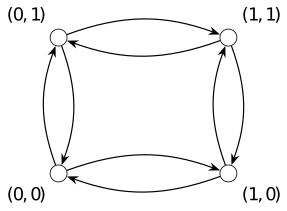
Each directed arc is one indexed edge. Horizontal and vertical arcs represent positive steps in the first and second coordinates, respectively; modulo two, both directions are positive coordinate steps. No face or plaquette constraint is imposed on the spatial link configurations in this example.
Take \(G=\mathbb Z_2\), written additively as \(\mathbb F_2\). A link configuration is \(u\in \mathbb F_2^{E_s}\), so \[\dim _{\mathbb C}\mathcal H_{\mathrm {link}}=2^8=256.\] A gauge function \(a\in \mathbb F_2^{V_s}\) acts by \[u_e\longmapsto u_e+a_{t(e)}+a_{s(e)}.\] The corresponding incidence map \(\delta :\mathbb F_2^{V_s}\to \mathbb F_2^{E_s}\) has kernel the constant functions: vanishing on every edge forces equal values along every path, and the graph is connected. Thus \(\dim \ker \delta =1\), \(\operatorname {rank}\delta =3\) and \(|\operatorname {im}\delta |=8\).
Every gauge orbit is a coset of \(\operatorname {im}\delta \), with 8 elements. The orbit basis therefore gives \[\dim _{\mathbb C}\mathcal H_{\mathrm {phys}} =\frac {256}{8}=32=2^5.\] The exponent is the cycle rank of this multigraph, \(b_1=|E_s|-|V_s|+1=8-4+1=5\). Equivalently, choose a spanning tree with three edges and set their additive link values to zero successively from a root. The remaining 5 chord values are free; the residual constant gauge function changes none of them. This supplies the same 32 representatives. The result counts neutral states of the link Hilbert space; it does not impose a flatness condition or identify opposite indexed edges.