Spatial Dirac operators [fdip-001C]
✍️sourceAGENTDRAFTED
- October 20, 2026
Spatial Dirac operators [fdip-001C]
✍️sourceAGENTDRAFTED
- October 20, 2026
A periodic spatial grid carries a different Clifford-module problem from the configuration space. A separately chosen complex Clifford module couples to centered differences. The square and Fourier blocks of the resulting Dirac operator can be calculated exactly. Its zero modes and comparison with nearest-neighbor differences show why a Clifford construction alone does not determine the desired kinetic operator or a continuum limit.
Definition 1. A centered Dirac operator on a finite periodic grid [fdip-000R]AGENTDRAFTED
- October 17, 2026
Definition 1. A centered Dirac operator on a finite periodic grid [fdip-000R]AGENTDRAFTED
- October 17, 2026
To couple Clifford multiplication to spatial differences, fix an integer \(d\ge 1\) and periods \(N_j\ge 3\) for \(1\le j\le d\). The periodic grid and its scalar fields are \[\begin {aligned} \Lambda &=\prod _{j=1}^d\mathbb Z/N_j\mathbb Z,\\ M&=\prod _{j=1}^d N_j,\qquad H=\mathbb C^\Lambda . \end {aligned}\] Write \(e_j\in \Lambda \) for the unit step in coordinate \(j\). Addition is periodic and the lattice spacing is one. Extend the counting pairing to the Hermitian inner product \[\langle f,g\rangle _H =\sum _{x\in \Lambda }\overline {f(x)}g(x),\] conjugate-linear in the first slot.
The spatial quadratic form is \[q_{\mathrm {sp}}(z)=\sum _{j=1}^d z_j^2 \qquad (z\in \mathbb C^d).\] It is distinct from the Hermitian norm squared \(\sum _j|z_j|^2\) and from the real four-field configuration form. For example, at \(i\varepsilon _1\), where \(\varepsilon _j\) is the standard basis of \(\mathbb C^d\), the quadratic value is \(-1\) and the Hermitian norm squared is \(1\). The grid steps \(e_j\), these complex coordinate vectors, and the 4 configuration coordinates have different carriers.
Choose \(S=(\mathbb C^2)^{\otimes d}\) with its standard tensor
basis and product Hermitian inner product. In the
Pauli convention, take
\[X=\begin {pmatrix}0&1\\1&0\end {pmatrix},\qquad
Z=\begin {pmatrix}1&0\\0&-1\end {pmatrix},\]
and put \(I=I_2\) and
\[\gamma _j=Z^{\otimes (j-1)}\otimes X
\otimes I^{\otimes (d-j)}.\]
An empty tensor product contributes the scalar identity.
Direct multiplication gives \(X^*=X\), \(Z^*=Z\),
\(X^2=Z^2=I\) and \(XZ=-ZX\). Ordinary tensor products obey
\[\begin {aligned}
(A\otimes B)^*&=A^*\otimes B^*,\\
(A\otimes B)(C\otimes E)&=AC\otimes BE.
\end {aligned}\]
The product formula follows on pure tensors, which span; the
adjoint formula follows from the product inner product on such
tensors. Thus \(\gamma _j^*=\gamma _j\) and
\(\gamma _j^2=I_S\). For \(i<j\), the only anticommuting slot is
\(i\), where \(X\) meets \(Z\). Before it both factors are \(Z\);
after it at least one factor is \(I\). Hence
\[\gamma _i\gamma _j+\gamma _j\gamma _i
=2\delta _{ij}I_S.\]
Mathlib's Matrix.kronecker,
Matrix.mul_kronecker_mul,
Matrix.conjTranspose_kronecker and
Matrix.one_kronecker_one give the corresponding
matrix construction and identities. Iterating them requires
identifying the product-index bases.
The complex-linear map \(c:\mathbb C^d\to \operatorname {End}_{\mathbb C}(S)\)
defined by \(c(z)=\sum _j z_j\gamma _j\) satisfies
\[\begin {aligned}
c(z)^2&=\sum _j z_j^2 I_S\\
&\quad +\sum _{i<j}z_i z_j
(\gamma _i\gamma _j+\gamma _j\gamma _i)\\
&=q_{\mathrm {sp}}(z)I_S.
\end {aligned}\]
The Clifford universal property therefore gives a
unique unital complex-algebra map
\[\begin {aligned}
\rho :\operatorname {Cl}(q_{\mathrm {sp}})&\longrightarrow
\operatorname {End}_{\mathbb C}(S),\\
\rho (\iota (\varepsilon _j))&=\gamma _j.
\end {aligned}\]
This makes \(S\) a Clifford module, in the
module-map convention.
The ordinary-algebra universal property is stated in
[meinrenken2013clifford, Proposition 2.2 and Remark 2.2, p. 29].
Its bilinear form is \(b(z,w)=\sum _j z_jw_j\), with relation
\(uv+vu=2b(u,v)1\); see
[meinrenken2013clifford, Definition 2.1, p. 27].
The displayed square identity is precisely the input required
by CliffordAlgebra.lift over \(\mathbb C\).
This chosen module is reducible. The involution \[J=I^{\otimes (d-1)}\otimes X\] commutes with every \(\gamma _j\): its last factor meets either \(I\) or \(X\), and its other factors are identities. Its two eigenspaces are \[S_\pm =(\mathbb C^2)^{\otimes (d-1)} \otimes \mathbb C(1,\pm 1).\] Both are nonzero and have dimension \(2^{d-1}\). Commutation with \(J\) makes them invariant under every generator and hence under the generated Clifford action. We use \(\dim S=2^d\); no minimality or faithfulness of this representation is needed.
Extend the cyclic shift coordinatewise: \[(T_j f)(x)=f(x+e_j).\] Its inverse shifts by \(-e_j\). Reindexing \(y=x+e_j\) gives \[\begin {aligned} \langle T_jf,g\rangle _H &=\sum _y\overline {f(y)}g(y-e_j)\\ &=\langle f,T_j^{-1}g\rangle _H. \end {aligned}\] Thus \(T_j^*=T_j^{-1}\), so \(T_j\) is unitary. The shifts and their inverses commute, since addition in \(\Lambda \) commutes. The centered differences are the endomorphisms \[\nabla _j=(T_j-T_j^{-1})/2.\] They commute and satisfy \(\nabla _j^*=-\nabla _j\). Their source and target are both \(H\), unlike a general vertex-to-edge incidence map.
Set \(K=S\otimes _{\mathbb C}H\), with \(\langle s\otimes f,t\otimes g\rangle _K =\langle s,t\rangle _S\langle f,g\rangle _H\). Identify \(s\otimes f\) with the field \(x\mapsto f(x)s\). The centered Dirac operator is \[D=\sum _{j=1}^d\gamma _j\otimes \nabla _j.\] Equivalently, \[\begin {aligned} (D\psi )(x) &=\frac 12\sum _{j=1}^d\gamma _j\psi (x+e_j)\\ &\quad -\frac 12\sum _{j=1}^d\gamma _j\psi (x-e_j). \end {aligned}\] For \(d=1\), this is \(X\) applied to the ordinary centered difference of a two-component field. Wingate's gauge-covariant centered difference reduces to this difference when all links are one and the spacing is one [wingate2025lattice, Section 9.1, Equation (9.2), p. 19]. The finite grid and tensor module here are specified directly; this construction introduces no Grassmann integration or gauge field. The Lorentz-sign gamma algebra is a different choice of form, scalar field and representation.
Theorem 2. The Dirac square and its finite Fourier blocks [fdip-000S]AGENTDRAFTED
- October 17, 2026
Theorem 2. The Dirac square and its finite Fourier blocks [fdip-000S]AGENTDRAFTED
- October 17, 2026
For the periodic grid and Clifford module, the centered Dirac operator is skew-adjoint and has square \[\begin {aligned} D^*&=-D,\\ D^2&=I_S\otimes \sum _{j=1}^d\nabla _j^2,\\ -D^2&=\frac 14 I_S\otimes \sum _{j=1}^d(2I_H-T_j^2-T_j^{-2}). \end {aligned}\] In particular \(-D^2=D^*D\) is positive semidefinite. Its complete finite Fourier decomposition has blocks \[\begin {aligned} D(p)&=i\sum _{j=1}^d\gamma _j\sin p_j,\\ -D(p)^2&=s(p)I_S,\\ s(p)&=\sum _{j=1}^d\sin ^2p_j, \end {aligned}\] where \(p_j=2\pi r_j/N_j\) and \(0\le r_j<N_j\). The sine convention agrees with the free propagator in [wingate2025lattice, Section 9.1, Equations (9.6)-(9.7), p. 20] after setting the spacing to one. The finite decomposition and square are proved below.
Proof.
- October 17, 2026
Proof.
- October 17, 2026
The tensor adjoint formula and \(\gamma _j^*=\gamma _j\), \(\nabla _j^*=-\nabla _j\) give \((\gamma _j\otimes \nabla _j)^* =-\gamma _j\otimes \nabla _j\); adding proves \(D^*=-D\). In the square, every diagonal term is \(\gamma _j^2\otimes \nabla _j^2=I_S\otimes \nabla _j^2\). For \(i<j\), the paired off-diagonal terms are \[\begin {gathered} \gamma _i\gamma _j\otimes \nabla _i\nabla _j +\gamma _j\gamma _i\otimes \nabla _j\nabla _i\\ =(\gamma _i\gamma _j+\gamma _j\gamma _i) \otimes \nabla _i\nabla _j=0, \end {gathered}\] using commutation of the differences and anticommutation of the distinct gamma matrices. This proves the square formula. Expanding \(\nabla _j^2\) gives \((T_j^2-2I_H+T_j^{-2})/4\). Finally \(\langle \psi ,-D^2\psi \rangle _K =\langle D\psi ,D\psi \rangle _K\ge 0\).
Let \(\mathcal R=\prod _j\{0,\ldots ,N_j-1\}\) and, for \(r\in \mathcal R\), define the normalized character function \[\chi _r(x)=M^{-1/2} \exp \left (i\sum _{j=1}^d p_jx_j\right ).\] Choose integer representatives for \(x_j\). Changing one by \(N_j\) multiplies the exponential by \(\exp (2\pi i r_j)=1\); changing \(r_j\) by \(N_j\) likewise multiplies it by \(\exp (2\pi i x_j)=1\). Thus the function depends only on the residue classes.
For \(r,t\in \mathcal R\), put \[\zeta _j=\exp \left (\frac {2\pi i(t_j-r_j)}{N_j}\right ).\] The counting inner product factors: \[\langle \chi _r,\chi _t\rangle _H =M^{-1}\prod _{j=1}^d\sum _{k=0}^{N_j-1}\zeta _j^k.\] If \(t_j=r_j\), then \(\zeta _j=1\) and the inner sum is \(N_j\). Otherwise the chosen range of labels gives \(\zeta _j\ne 1\) and \(\zeta _j^{N_j}=1\), so \[(1-\zeta _j)\sum _{k=0}^{N_j-1}\zeta _j^k =1-\zeta _j^{N_j}=0.\] Division by \(1-\zeta _j\) makes that sum zero. Consequently \(\langle \chi _r,\chi _t\rangle _H=\delta _{rt}\). There are \(M\) such functions, and \(\dim _{\mathbb C}H=M\), as witnessed by the vertex indicators. Orthonormality gives linear independence, so these functions form a complete basis.
For a spinor-valued field, the Fourier transform and inverse therefore are \[\begin {aligned} \widehat \psi (r) &=M^{-1/2}\sum _{x\in \Lambda } e^{-i\sum _jp_jx_j}\psi (x),\\ \psi (x) &=M^{-1/2}\sum _{r\in \mathcal R} e^{i\sum _jp_jx_j}\widehat \psi (r). \end {aligned}\] For scalar fields the coefficient is \(\widehat f(r)=\langle \chi _r,f\rangle _H\); applying that basis expansion in each standard coordinate of \(S\) proves the two vector-valued formulas. Thus \[K=\bigoplus _{r\in \mathcal R} S\otimes \mathbb C\chi _r.\] The forward shift has \(T_j\chi _r=e^{ip_j}\chi _r\), hence \(\nabla _j\chi _r=i\sin p_j\,\chi _r\). Each displayed summand is invariant under \(D\), with block \(D(p)=i\sum _j\gamma _j\sin p_j\). Expanding its square using the same anticommutators gives \(D(p)^2=-s(p)I_S\).
Mathlib's LinearMap.adjoint and
LinearMap.adjoint_inner_right give the finite-dimensional
adjoint and its characterizing identity;
LinearMap.adjoint_comp reverses composition.
The relevant formal inner-product structure is the counting
Euclidean space, for example a \(\operatorname {PiLp}(2)\)
model. The raw function type's default supremum norm cannot
silently replace that structure. The translation and tensor
identifications are the direct calculations above.
Mathlib's ZMod.dft,
ZMod.dft_apply and ZMod.invDFT_apply
provide the one-coordinate Fourier equivalence: its forward
sum has a negative exponent and no normalizing factor, while
its inverse has a positive exponent and factor \(N^{-1}\).
Iterating over coordinates and scaling the forward transform
by \(M^{-1/2}\) gives the conventions above.
AddChar.wInner_cWeight_eq_boole gives generic
character orthogonality for the normalized average inner
product. Here the unscaled characters have counting norm
\(\sqrt M\); the factor \(M^{-1/2}\) makes them orthonormal.
Their explicit enumeration, the shift eigenvalues and the
spinor blocks are supplied by this finite proof.
Proposition 3. Zero modes and the nearest-neighbor mismatch [fdip-000T]AGENTDRAFTED
- October 17, 2026
Proposition 3. Zero modes and the nearest-neighbor mismatch [fdip-000T]AGENTDRAFTED
- October 17, 2026
On the periodic grid, let \(e\) be the number of even periods among \(N_1,\ldots ,N_d\). The centered Dirac operator has exactly \(2^e\) zero momentum blocks and \[\dim _{\mathbb C}\ker D=2^{d+e}.\] This is the kernel dimension for the explicitly chosen reducible module \(S\), whose dimension is \(2^d\). The unit-weight graph Laplacian \[L_{\mathrm {nn}}=\sum _{j=1}^d (2I_H-T_j-T_j^{-1})\] has only the zero momentum in its scalar kernel. Moreover \(-D^2\ne I_S\otimes L_{\mathrm {nn}}\) on every permitted grid, including grids with all periods odd. These are finite consequences of the Fourier blocks; the centered-difference convention comes from [wingate2025lattice, Section 9.1, Equations (9.2), (9.6)-(9.7), pp. 19-20].
Proof.
- October 17, 2026
Proof.
- October 17, 2026
The forward-difference factorization from Lemma [fdip-0014], applied in each coordinate, gives \[L_{\mathrm {nn}}=\sum _j(T_j-I_H)^*(T_j-I_H).\] For \(N_j\ge 3\), each undirected nearest-neighbor edge occurs once in the corresponding squared-difference energy. On the character with momentum \(p\), the eigenvalue is \[\begin {aligned} \ell (p)&=\sum _j(2-2\cos p_j)\\ &=4\sum _j\sin ^2(p_j/2). \end {aligned}\] The positive Dirac square has scalar block \(s(p)=\sum _j\sin ^2p_j\). The double-angle identity gives \[\ell (p)-s(p)=4\sum _j\sin ^4(p_j/2).\] Choose \(r_1=1\) and the other labels zero. Since \(N_1\ge 3\), \(\sin (\pi/N_1)>0\), so the difference is strictly positive on that block. This proves the operator mismatch.
Every summand of \(s(p)\) is nonnegative. Hence \(s(p)=0\) exactly when each \(\sin p_j=0\). In the range \(0\le r_j<N_j\), this means \(r_j=0\), or \(r_j=N_j/2\) when \(N_j\) is even. There are exactly \(2^e\) choices. On each such block \(D(p)=0\) on all of \(S\). Every other block is invertible, with two-sided inverse \[D(p)^{-1}=-D(p)/s(p),\] because \(D(p)^2=-s(p)I_S\). Completeness of the Fourier basis therefore gives \(\dim \ker D=2^e\dim S=2^{d+e}\). In contrast, \(\ell (p)=0\) forces \(r_j=0\) for every \(j\); thus \(\dim \ker (I_S\otimes L_{\mathrm {nn}})=2^d\).
For \(d=1,N=4\), the alternating scalar field \(a(x)=(-1)^x\) has momentum \(p=\pi \). Its centered difference is zero, whereas \(L_{\mathrm {nn}}a=4a\). Consequently every field \(x\mapsto a(x)v\), \(v\in S\), is killed by \(D\). Together with the constant fields these give the four-dimensional kernel. Write \(K_2=(2I_H-T^2-T^{-2})/4\), so \(-D^2=I_S\otimes K_2\). The two scalar Laplacians have the following weighted graphs:
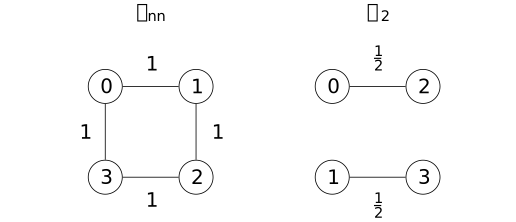
Left: the 4 unit-weight nearest-neighbor edges. Right: the two-step edges, with vertices rearranged to display the parity classes \(\{0,2\}\) and \(\{1,3\}\). At period \(4\), \(T^2=T^{-2}\), so \(K_2=(I_H-T^2)/2\): the two shift contributions of weight \(1/4\) combine into one undirected edge of weight \(1/2\) for each opposite pair. The alternating field is constant on each right-hand component, explaining its zero energy there.
For \(d=1,N=3\), momentum \(p=2\pi/3\) instead gives \[s(p)=\tfrac 34,\qquad \ell (p)=3.\] Only \(r=0\) is a zero momentum, yet the operators still differ. Thus extra exact zero momenta occur precisely when at least one period is even, whereas the square mismatch always occurs. The excluded case \(N=2\) has \(T=T^{-1}\), making its centered difference identically zero.
The finite kernel dimension above is not a physical species or chirality count. Friedan's Nielsen-Ninomiya theorem concerns free fermions on the infinite lattice \(\mathbb Z^d\) for odd \(d\), with continuous torus momenta. Its Hamiltonian is quadratic, phase invariant, translation invariant and local, with a Hermitian momentum symbol. The locality discussion reduces the Hamiltonian requirement to continuity; the internal-charge projections must be smooth. The zero set is finite and isolated, with specified relativistic Clifford-linear behavior near each zero. Under these hypotheses the total chiral index vanishes separately for each charge [friedan1982nielsen, Sections 1-2, pp. 481-484; Equations (6), (10)-(11)]. A finite sampled grid in arbitrary dimension with the chosen reducible module computes a different quantity. The odd-period example neither contradicts that theorem nor establishes a continuum limit. No Lorentzian model or factorization of the earlier weighted precision is supplied by this centered operator.