Example. Cycle decimation and periodic covariance [fdip-0057]
AGENTDRAFTED
Take the unit-weight cycle on \(\mathbb Z/(2N)\), with
\(N\ge 3\) and precision \(Q=L_{C_{2N}}+aI\), where
\(a=m^2>0\). The group \(G=C_N\) acts by two-site rotations.
It preserves the even retained vertices and the odd eliminated
vertices. Write \(x_j=\phi _{2j}\), \(y_j=\phi _{2j+1}\) and
\(q=2+a\); indices \(j\) lie in \(\mathbb Z/N\).
For the shift \((Tz)_j=z_{j-1}\), the blocks are
\[A=C=qI,\qquad B=-(I+T),\qquad B^*=-(I+T^{-1}).\]
Thus the equivariant Schur formula gives
\[\begin {aligned}
S&=qI-q^{-1}(2I+T+T^{-1})\\
&=w'L_{C_N}+a'I,\\
w'&=\frac 1{2+a},\qquad
a'=(2+a)-\frac 4{2+a}
=\frac {a(a+4)}{a+2}>0.
\end {aligned}\]
Here \(L_{C_N}=2I-T-T^{-1}\). The restriction \(Q_{RR}=qI\)
has no off-diagonal entries, while \(S\) has entries \(-1/q\)
between adjacent retained vertices. The retained set is stable under
\(G\), but the marginal precision is induced by elimination.
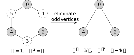
The six-cycle illustrates \(N=3\). Shaded even vertices remain;
dashed odd vertices are integrated out. Each triangle edge has
weight \(1/q\), and the mass squared changes from \(a\) to
\(q-4/q\), with \(q=2+a\).
The finite Gaussian normalization is retained exactly:
\(Z_Q=Z_CZ_S\) with \(Z_C=(2\pi/q)^{N/2}\), and the retained
law is \(\mu _S\). The effective weight and mass are both part of
this law. Dividing \(S\) by \(w'\) is useful for comparing its
parameters, but changes the field covariance by a scalar unless
the corresponding field rescaling is also made.
Put \(q=2\cosh \omega \) with \(\omega >0\). Then
\[2+\frac {a'}{w'}=q^2-2=2\cosh (2\omega ).\]
The doubled parameter has an exact finite-ring interpretation.
For \(M\ge 3\), the covariance of precision
\(w(2\cosh \eta \,I-T-T^{-1})\) on \(\mathbb Z/M\), with
\(w,\eta >0\), is the periodic kernel
\[\begin {aligned}
K_{M,w,\eta }(r)
&=\frac {e^{-\eta r}+e^{-\eta (M-r)}}
{2w\sinh \eta \,(1-e^{-M\eta })},\\
&\hspace {24mm}0\le r\le M-1.
\end {aligned}\]
For the original and retained fields this gives
\[(Q^{-1})_{0,2r}
=K_{2N,1,\omega }(2r)
=K_{N,w',2\omega }(r)
=(S^{-1})_{0,r}.\]
The equality is between covariances with their actual weights.
In the convention that correlation length is the reciprocal decay
rate of these periodized exponential images, it changes from
\(\xi =1/\omega \) fine lattice units to
\(\xi '=1/(2\omega )=\xi / 2\) coarse lattice units. The finite ring
has two winding directions, so its covariance is not a single
exponential in separation. If the old spacing is \(\ell \), the new
spacing is \(2\ell \); the physical decay length
\(\ell / \omega =(2\ell )/(2\omega )\) is unchanged.
The bound \(N\ge 3\) keeps the reduced graph a simple cycle.
At \(N=2\), \(T=T^{-1}\) and two eliminated vertices connect the
same retained pair, producing two parallel edges of weight \(1/q\),
or one edge of weight \(2/q\). At \(a=0\), the algebraic formula
still gives \(w'=1/2\) and \(a'=0\), the two-resistors-in-series
limit. The full precision then has a constant zero mode and no
normalized full-space Gaussian law. Pinning or a mean-zero
constraint must be specified as in
constrained massless laws; the positive-mass covariance
formula is not a finite limit on the full field space.
This is a direct cycle calculation within
Kron reduction, the Schur reduction of graph Laplacians
with possible positive diagonal terms.
Closure follows from [dorfler2011kron, Lemma 2.1, pp. 5-6].
Successive and simultaneous eliminations agree by
[dorfler2011kron, Lemma 3.3, p. 14].
In that source the diagonal mass corresponds to a
shunt conductance or graph self-loop. In the incidence convention
used here an edge with identical endpoints has zero difference;
the mass is therefore kept as the separate term \(aI\).
The source supplies the general reduction context, while the
periodic covariance and scale statements are proved above.