Gaussian laws over symmetry sectors [fdip-0054]
✍️sourceAGENTDRAFTED
- November 1, 2026
Gaussian laws over symmetry sectors [fdip-0054]
✍️sourceAGENTDRAFTED
- November 1, 2026
The real isotypic projectors split a field space, and the positive multiplicity matrices describe its symmetry-preserving precisions. For a real Gaussian field this becomes a product of independent sector laws, with real dimensions and normalizers fixed by the scalar type. The result extends the two-sector product law.
If the retained vertices form a union of group orbits, elimination can be performed separately in each sector. Symmetry survives, but the retained precision can change: keeping every other vertex of a cycle produces a new cycle with different weight and mass. Its exact periodic covariance explains the change of decay scale without identifying a finite ring with an infinite lattice.
Theorem 1. Independent Gaussian laws on real isotypic sectors [fdip-0055]AGENTDRAFTED
- November 1, 2026
Theorem 1. Independent Gaussian laws on real isotypic sectors [fdip-0055]AGENTDRAFTED
- November 1, 2026
Let a finite group \(G\) act orthogonally on a finite-dimensional real inner-product space \(H\), and let \(Q>0\) be self-adjoint and \(G\)-equivariant. Write the orthogonal isotypic projectors as \(E_\Xi \), put \(H_\Xi =E_\Xi H\), and omit the zero sectors. Use induced Euclidean volumes and uncompleted Borel sigma-algebras. For the normalized Gaussian law \(\mu _Q\), the map \[\mathcal D:H\longrightarrow \prod _\Xi H_\Xi , \qquad z\longmapsto (E_\Xi z)_\Xi \] satisfies \[\mathcal D_*\mu _Q=\bigotimes _\Xi \mu _{Q|_{H_\Xi }}. \qquad Z_Q=\prod _\Xi Z_{Q|_{H_\Xi }}.\] Thus the projected fields are independent. Each has covariance \((Q|_{H_\Xi })^{-1}\) on its own real sector.
In the multiplicity coordinates, set \(D_\Xi =\operatorname {End}_G(W_\Xi )\), \(r_\Xi =\dim _{D_\Xi }W_\Xi \), and \(d_\Xi =\dim _{\mathbb R}D_\Xi \in \{1,2,4\}\). Write \(Q_\Xi \in M_{m_\Xi }(D_\Xi )\) for the multiplicity matrix; it is not the entire real-sector matrix. Then \[\begin {aligned} \det _{\mathbb R}Q &=\prod _\Xi \det _{\mathbb R} (Q_\Xi :D_\Xi ^{m_\Xi }\to D_\Xi ^{m_\Xi })^{r_\Xi },\\ Z_{Q|_{H_\Xi }} &=\frac {(2\pi )^{m_\Xi r_\Xi d_\Xi/2}} {\det _{\mathbb R}(Q_\Xi )^{r_\Xi/2}}. \end {aligned}\] The determinants in these formulas are ordinary determinants of real linear operators, including when \(D_\Xi =\mathbb H\).
Proof.
- November 1, 2026
Proof.
- November 1, 2026
The projectors are self-adjoint, mutually orthogonal and sum to \(I\). Addition from the product of their images is an isometry inverse to \(\mathcal D\). Concatenated orthonormal bases identify the orthogonal product volume with volume on \(H\); finite products of these Borel spaces have the product Borel sigma-algebra. Commutation with every projector makes \(Q\) block diagonal, so its positive quadratic form is the sum of its sector quadratic forms. The exponential weight therefore factors.
Each restricted precision is positive, and the Gaussian normalizer theorem makes every sector integral finite and positive. Nonnegative Tonelli gives the product of normalizers. Integrating the factored density on a Borel rectangle gives the product of its sector probabilities; uniqueness of finite measures on the rectangle-generated sigma-algebra gives the stated product law. This is the same measure argument as in Theorem [fdip-000M], now for the finite family of projectors. The inverse-precision covariance theorem applies to each factor. Empty sectors have unit normalizer and their one-point law.
For the determinant, the real-sector matrix is the direct sum of \(r_\Xi \) identical real operators \(Q_\Xi \) on \(D_\Xi ^{m_\Xi }\), by the orthonormal scalar-column construction of Corollary [fdip-0050]. Determinants multiply under real direct sums. If the positive Hermitian eigenvalues of \(Q_\Xi \) are \(\lambda _1,\ldots ,\lambda _{m_\Xi }\), its real determinant is \(\prod _j\lambda _j^{d_\Xi }\). Substitution into the real Gaussian normalizer gives the displayed formula.
For the twisted prism, the trivial multiplicity matrix has determinant \(4\), while the complex matrix has complex determinant \(46\). Both have \(r_\Xi =1\), so \(\det _{\mathbb R}Q=4\cdot 46^2=8464\) and \(Z_Q=(2\pi )^3/92\). For the binary tetrahedral Cayley graph, write \(a=m^2>0\). The 5 real sectors give the following factors: \[\begin {array}{c|c|c} D_\Xi &r_\Xi &\det _{\mathbb R}(Q|_{H_\Xi })\\\hline \mathbb R&1&a\\ \mathbb C&1&(a+3)^2\\ \mathbb R&3&[(a+8)(a+11)^2]^3\\ \mathbb H&1&(a+9)^4\\ \mathbb C&2&[(a+6)(a+9)]^4 \end {array}\] Their product is \[\det _{\mathbb R}Q =a(a+3)^2(a+6)^4(a+8)^3(a+9)^8(a+11)^6.\] The exponents sum to \(24\), the real field dimension. The normalizer is \[Z_Q=\frac {(2\pi )^{12}}{\sqrt {\det _{\mathbb R}Q}}.\] These factors use the mass-shifted precision, not the singular Laplacian alone.
The density convention agrees with [friedli2017statistical, Theorem 8.4, p. 385] after setting its mean to zero and its covariance to \(\Sigma =Q^{-1}\). That theorem identifies the Gaussian density; the finite-group projectors and real determinant exponents are supplied by the proofs above and in Corollary [fdip-0050].
Mathlib's
ProbabilityTheory.HasGaussianLaw.iIndepFun_of_covariance_inner
supports the independence step for a finite family of jointly
Gaussian real Hilbert-space variables. Here the family is
\(z\mapsto (E_\Xi z)_\Xi \), a linear image of the Gaussian field.
For distinct sectors and \(u\in H_\Xi \), \(v\in H_\Psi \), its
scalar cross covariance is \(\langle u,Q^{-1}v\rangle =0\),
because \(Q^{-1}\) preserves the orthogonal sectors. Thus the
declaration's zero-cross-covariance hypothesis matches this family.
It does not assert the representation-theoretic decomposition or the
real determinant exponents.
Theorem 2. Equivariant elimination within each sector [fdip-0056]AGENTDRAFTED
- November 1, 2026
Theorem 2. Equivariant elimination within each sector [fdip-0056]AGENTDRAFTED
- November 1, 2026
Let \(H=X\mathbin \perp Y\) be a finite-dimensional orthogonal real representation of a finite group \(G\), with both summands \(G\)-stable. Let the positive self-adjoint equivariant precision be \[Q=\begin {pmatrix}A&B\\B^*&C\end {pmatrix}, \qquad B:Y\to X.\] Then \(C>0\), and the retained precision \(S=A-BC^{-1}B^*:X\to X\) is positive, self-adjoint and \(G\)-equivariant. For every real irreducible type \(\Xi \), set \(X_\Xi =E_\Xi X\) and \(Y_\Xi =E_\Xi Y\). All block maps restrict to the indicated source and target sectors, and \[S|_{X_\Xi } =A|_{X_\Xi }-B_\Xi (C|_{Y_\Xi })^{-1}B_\Xi ^*.\] In common multiplicity coordinates, the same formula is \[S_\Xi =A_\Xi -B_\Xi C_\Xi ^{-1}B_\Xi ^*,\] where \(B_\Xi \) is an \(m_{X,\Xi }\times m_{Y,\Xi }\) matrix over \(D_\Xi \), and the products retain their displayed order.
Proof.
- November 1, 2026
Proof.
- November 1, 2026
Let \(\rho _X,\rho _Y\) denote the actions on the two summands. Equivariance of \(Q\) gives \(A\rho _X(g)=\rho _X(g)A\), \(B\rho _Y(g)=\rho _X(g)B\), and \(C\rho _Y(g)=\rho _Y(g)C\), together with the adjoint identity for \(B^*\). Positivity on \((0,y)\) makes \(C\) positive and invertible. Its inverse commutes with \(\rho _Y(g)\) by multiplying the commuting identity by \(C^{-1}\) on both sides. Hence the composite \(BC^{-1}B^*:X\to X\) and \(S\) commute with \(\rho _X(g)\). The same relations hold for the projectors, since they are real linear combinations of group actions.
Consequently \(B^*\) takes \(X_\Xi \) to \(Y_\Xi \), \(C^{-1}\) preserves \(Y_\Xi \), and \(B\) takes \(Y_\Xi \) back to \(X_\Xi \). The restriction of \(C^{-1}\) is the inverse of the restriction of \(C\), by restricting both inverse identities. This proves the typed formula, extending Proposition [fdip-003Q]. Choose isometric copies of the same real irreducible in \(X_\Xi \) and \(Y_\Xi \). Intertwiners then become rectangular matrices over \(D_\Xi \) and composition becomes ordered matrix multiplication, with adjunction given by conjugate transpose. This proves the multiplicity formula also over \(\mathbb H\); no scalar factors have been commuted. An absent \(Y_\Xi \) contributes a zero composite.
Completing the real square gives \[\begin {aligned} \langle (x,y),Q(x,y)\rangle &=\langle x,Sx\rangle \\ &\quad +\langle y+C^{-1}B^*x, C(y+C^{-1}B^*x)\rangle . \end {aligned}\] Testing at \(y=-C^{-1}B^*x\) proves \(S>0\); its self-adjointness follows by adjointing the composite. This uses the real inner product, regardless of the scalar algebra of a multiplicity matrix.
Use induced Euclidean volumes and let \(\pi :H\to X\) be the orthogonal projection. For every fixed \(x\), translation in \(Y\) and the completed square give \[\int _Y e^{-\langle (x,y),Q(x,y)\rangle/2}\,d\lambda _Y(y) =Z_Ce^{-\langle x,Sx\rangle/2}.\] Nonnegative Tonelli and normalization therefore give \(Z_Q=Z_CZ_S\) and \(\pi _*\mu _Q=\mu _S\), as in positive elimination. Applying the same argument in \(X_\Xi \mathbin \perp Y_\Xi \), and then the sector product law, gives \[\begin {aligned} (\mathcal D_X)_*\pi _*\mu _Q &=\bigotimes _\Xi \mu _{S|_{X_\Xi }},\\ (\pi _\Xi )_*\mu _{Q|_{H_\Xi }} &=\mu _{S|_{X_\Xi }},\qquad Z_C=\prod _\Xi Z_{C|_{Y_\Xi }}. \end {aligned}\] Here \(\pi _\Xi :H_\Xi \to X_\Xi \); the identity \(\pi E_\Xi =E_\Xi \pi \) shows that decomposing and projecting commute as maps. Product measures then give the same commuting square as in Theorem [fdip-003R], with all real isotypic sectors in place of the two sign sectors.
For vertex fields, the hypothesis holds when the retained set \(R\) is \(G\)-stable: take \(X=\mathbb R^R\) and \(Y=\mathbb R^{V\setminus R}\). It asserts equivariance of the induced marginal law. It does not assert that \(S=A\), the compressed precision. The cycle decimation gives a \(G\)-stable retained set with a nonzero Schur correction.
Example 3. Cycle decimation and periodic covariance [fdip-0057]AGENTDRAFTED
- November 1, 2026
Example 3. Cycle decimation and periodic covariance [fdip-0057]AGENTDRAFTED
- November 1, 2026
Take the unit-weight cycle on \(\mathbb Z/(2N)\), with \(N\ge 3\) and precision \(Q=L_{C_{2N}}+aI\), where \(a=m^2>0\). The group \(G=C_N\) acts by two-site rotations. It preserves the even retained vertices and the odd eliminated vertices. Write \(x_j=\phi _{2j}\), \(y_j=\phi _{2j+1}\) and \(q=2+a\); indices \(j\) lie in \(\mathbb Z/N\). For the shift \((Tz)_j=z_{j-1}\), the blocks are \[A=C=qI,\qquad B=-(I+T),\qquad B^*=-(I+T^{-1}).\] Thus the equivariant Schur formula gives \[\begin {aligned} S&=qI-q^{-1}(2I+T+T^{-1})\\ &=w'L_{C_N}+a'I,\\ w'&=\frac 1{2+a},\qquad a'=(2+a)-\frac 4{2+a} =\frac {a(a+4)}{a+2}>0. \end {aligned}\] Here \(L_{C_N}=2I-T-T^{-1}\). The restriction \(Q_{RR}=qI\) has no off-diagonal entries, while \(S\) has entries \(-1/q\) between adjacent retained vertices. The retained set is stable under \(G\), but the marginal precision is induced by elimination.
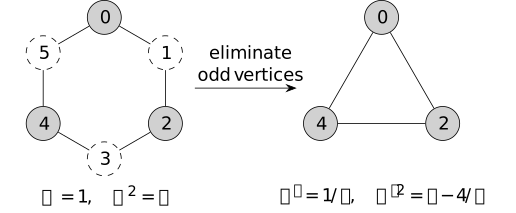
The six-cycle illustrates \(N=3\). Shaded even vertices remain; dashed odd vertices are integrated out. Each triangle edge has weight \(1/q\), and the mass squared changes from \(a\) to \(q-4/q\), with \(q=2+a\).
The finite Gaussian normalization is retained exactly: \(Z_Q=Z_CZ_S\) with \(Z_C=(2\pi/q)^{N/2}\), and the retained law is \(\mu _S\). The effective weight and mass are both part of this law. Dividing \(S\) by \(w'\) is useful for comparing its parameters, but changes the field covariance by a scalar unless the corresponding field rescaling is also made.
Put \(q=2\cosh \omega \) with \(\omega >0\). Then \[2+\frac {a'}{w'}=q^2-2=2\cosh (2\omega ).\] The doubled parameter has an exact finite-ring interpretation. For \(M\ge 3\), the covariance of precision \(w(2\cosh \eta \,I-T-T^{-1})\) on \(\mathbb Z/M\), with \(w,\eta >0\), is the periodic kernel \[\begin {aligned} K_{M,w,\eta }(r) &=\frac {e^{-\eta r}+e^{-\eta (M-r)}} {2w\sinh \eta \,(1-e^{-M\eta })},\\ &\hspace {24mm}0\le r\le M-1. \end {aligned}\] For the original and retained fields this gives \[(Q^{-1})_{0,2r} =K_{2N,1,\omega }(2r) =K_{N,w',2\omega }(r) =(S^{-1})_{0,r}.\] The equality is between covariances with their actual weights.
Proof.
- November 1, 2026
Proof.
- November 1, 2026
On the integer line, put \(h(n)=e^{-\eta |n|}/(2w\sinh \eta )\). For \(n\ne 0\), the two geometric progressions give \(w(2\cosh \eta \,h(n)-h(n-1)-h(n+1))=0\). At \(n=0\) the expression equals \((2\cosh \eta -2e^{-\eta })/(2\sinh \eta )=1\). Periodize this identity by summing \(h(r+kM)\) over \(k\in \mathbb Z\); absolute convergence permits the finite difference operation under the sum. The result is the unit point source on \(\mathbb Z/M\), so the periodized kernel is the inverse of the positive precision. Summing the geometric series gives \(K_{M,w,\eta }\).
For \(M=2N\) and even separation \(2r\), the numerator and periodic denominator equal those for \(M=N\), \(\eta =2\omega \). Their remaining constants agree because \[2w'\sinh (2\omega ) =\frac {2\sinh (2\omega )}{2\cosh \omega } =2\sinh \omega .\] This proves the covariance identity directly, in agreement with Gaussian marginalization.
In the convention that correlation length is the reciprocal decay rate of these periodized exponential images, it changes from \(\xi =1/\omega \) fine lattice units to \(\xi '=1/(2\omega )=\xi / 2\) coarse lattice units. The finite ring has two winding directions, so its covariance is not a single exponential in separation. If the old spacing is \(\ell \), the new spacing is \(2\ell \); the physical decay length \(\ell / \omega =(2\ell )/(2\omega )\) is unchanged.
The bound \(N\ge 3\) keeps the reduced graph a simple cycle. At \(N=2\), \(T=T^{-1}\) and two eliminated vertices connect the same retained pair, producing two parallel edges of weight \(1/q\), or one edge of weight \(2/q\). At \(a=0\), the algebraic formula still gives \(w'=1/2\) and \(a'=0\), the two-resistors-in-series limit. The full precision then has a constant zero mode and no normalized full-space Gaussian law. Pinning or a mean-zero constraint must be specified as in constrained massless laws; the positive-mass covariance formula is not a finite limit on the full field space.
This is a direct cycle calculation within Kron reduction, the Schur reduction of graph Laplacians with possible positive diagonal terms. Closure follows from [dorfler2011kron, Lemma 2.1, pp. 5-6]. Successive and simultaneous eliminations agree by [dorfler2011kron, Lemma 3.3, p. 14]. In that source the diagonal mass corresponds to a shunt conductance or graph self-loop. In the incidence convention used here an edge with identical endpoints has zero difference; the mass is therefore kept as the separate term \(aI\). The source supplies the general reduction context, while the periodic covariance and scale statements are proved above.
Remark 4. Symmetry of a marginal and restriction of a precision [fdip-0058]AGENTDRAFTED
- November 1, 2026
Remark 4. Symmetry of a marginal and restriction of a precision [fdip-0058]AGENTDRAFTED
- November 1, 2026
The sector laws use an ordinary orthogonal finite-group action on a real field space and a strictly positive precision. These hypotheses allow independent Gaussian factors and equivariant elimination. They do not make every stable retained subspace a reducing subspace for the precision. A stable vertex set says that its coordinate projection commutes with the group action; cycle decimation shows that it need not commute with \(Q\). The resulting Schur precision can therefore differ from the compression \(Q_{RR}\). Commuting with the group action and commuting with \(Q\) are distinct conditions.
Three other representation-theoretic questions need additional data. Projective representations and twisted group algebras record a multiplier rather than an ordinary group action; the projective obstruction explains its role. Restriction to a normal subgroup and Clifford's homogeneity theorem concern constituents under a specified subgroup inclusion; this is Clifford theory of group representations, distinct from Clifford algebras. In positive characteristic, the averaging denominator or Gaussian measure used here may be absent. None of these is supplied by real isotypic factorization alone.