Selected backgrounds and invariants [fdip-0059]
✍️sourceAGENTDRAFTED
- November 1, 2026
Selected backgrounds and invariants [fdip-0059]
✍️sourceAGENTDRAFTED
- November 1, 2026
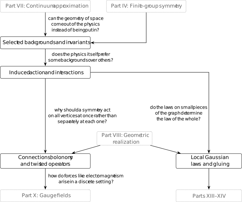
Can geometry be induced instead of supplied? Edge weights set the stiffness of field differences and may encode geometric information; they are not universally distances. Comparing choices through an induced action first requires keeping the graph data distinct from the choice of which field to retain. A retained field need not consist of named vertex coordinates. It may be a symmetry sector, or another specified subspace of the vertex fields. An orthogonal projector records this choice relative to the counting metric. Integrating out its orthogonal complement produces a Gaussian law on the chosen subspace.
The graph and its selector remain separate data. A graph relabeling must transport both, while an arbitrary orthogonal comparison of precisions can forget incidence. The examples below compare three selectors on one four-cycle and two rank-4 selectors on a quaternion Cayley graph. Their retained spectra separate choices that the unselected graph cannot distinguish. The restriction criterion then identifies exactly when eliminating the complement changes the compressed precision; a stable prism line shows why group symmetry alone is insufficient. In this chapter \(\Gamma \) denotes a symmetry group and \(G=Q^{-1}\) denotes the Green operator.
Definition 1. A selected Gaussian background [fdip-005A]AGENTDRAFTED
- November 1, 2026
Definition 1. A selected Gaussian background [fdip-005A]AGENTDRAFTED
- November 1, 2026
A selected Gaussian background is a tuple \[b=(\Pi ,w,m,P),\qquad \Pi =(V,E,s,h),\] where \(\Pi \) is a finite incidence presentation, \(w:E\to \mathbb R_{>0}\), \(m>0\), and \(P\) is an orthogonal projector on the counting inner-product space \(H=\mathbb R^V\), with \[P^2=P=P^*,\qquad 0<\operatorname {rank}P<|V|.\] The selected space is \(X=\operatorname {im}P\), its orthogonal complement is \(Y=\ker P\), and the observed random vector is \(P\phi \in X\). Incidence, the Green operator and the full law are \[\begin {aligned} (d\phi )(e)&=\phi (h(e))-\phi (s(e)),\\ Q&=d^*Wd+m^2I>0,\qquad G=Q^{-1},\\ \phi &\sim \mu _Q. \end {aligned}\] Here \(W=\operatorname {diag}(w)\) and \(\mu _Q\) uses the induced Euclidean volume. These are derived from the tuple, not additional choices.
Three constructions supply such projectors, provided their ranks are nonzero and proper.
- A retained subset \(R\subsetneq V\) gives \(P_R\phi =\sum _{v\in R}\phi (v)\delta _v\). Identifying \(\operatorname {im}P_R\) with \(\mathbb R^R\) recovers the coordinate background.
- A finite signed graph symmetry \(\rho :\Gamma \to O(H)\) extends to \(\mathbb R[\Gamma ]\). For \(e^2=e=e^*\), where \([g]^*=[g^{-1}]\), \(P=\rho (e)\) is orthogonal because \(\rho (e)^*=\rho (e^*)\). The precision commutes with every \(\rho (g)\), hence with this \(P\).
- For a \(\Gamma \)-stable subspace \(X\subset H\), its orthogonal projector commutes with \(\rho (\Gamma )\): orthogonality makes \(X^\perp \) stable too. It need not commute with \(Q\). Within a repeated real isotypic block, the chosen multiplicity subspace may fail to be invariant under the positive multiplicity matrix. These are different constructions: a subrepresentation projector commutes with \(\rho (\Gamma )\) but need not commute with \(Q\); a group-algebra projector commutes with \(Q\) but need not commute with \(\rho (\Gamma )\). Centrality of \(e\) is sufficient for the latter commutation, and hence for a stable image.
Every subspace has a unique orthogonal projector for the specified metric. This makes the selector equivalent to choosing \(X\), without choosing an additional complementary subspace. An oblique idempotent \(T^2=T\) also gives a Gaussian observation \(T\phi \), and orthogonal conjugation does transport it naturally: \(T\mapsto OTO^{-1}\). But it also records a possibly nonorthogonal kernel, so the image alone no longer determines the observation or its covariance \(TGT^*\). General linear observations are outside this definition. No physical rule selecting \(P\) from an environment is assumed.
Theorem 2. The law on a selected subspace [fdip-005B]AGENTDRAFTED
- November 1, 2026
Theorem 2. The law on a selected subspace [fdip-005B]AGENTDRAFTED
- November 1, 2026
For a selected background, view \(P\) as a map \(H\to X=\operatorname {im}P\) and let \(r=\dim X\). The law \(\nu _b=P_*\mu _Q\) is the centered Gaussian on \(X\) with intrinsic covariance and precision \[C_P=(PGP)|_X>0,\qquad S_P=C_P^{-1}:X\to X.\] Relative to the induced Euclidean volume \(\lambda _X\), its density is \[\frac {d\nu _b}{d\lambda _X}(x) =\frac {\sqrt {\det _X S_P}}{(2\pi )^{r/2}} e^{-\langle x,S_Px\rangle /2}.\] If \(B:\mathbb R^r\to H\) is an isometric inclusion with image \(X\), then \(BB^*=P\); its chosen coordinate matrices are \[B^*C_PB=B^*GB,\qquad [S_P]_B=(B^*GB)^{-1}.\] For another such basis \(B'=BU\), \(U\in O(r)\), the latter changes to \(U^*[S_P]_BU\). The intrinsic operator \(S_P\) is independent of this choice.
Proof.
- November 1, 2026
Proof.
- November 1, 2026
For nonzero \(x\in X\), \(\langle x,C_Px\rangle =\langle x,Gx\rangle >0\). Set \(C=B^*GB\), so \(C>0\). The positive square roots of \(Q\) and \(C\) exist by the real spectral theorem. The density change of variables \(z=Q^{1/2}\phi \) gives the standard Gaussian density \((2\pi )^{-|V|/2}e^{-|z|^2/2}\): its Jacobian and the normalizer cancel. Put \[T=C^{-1/2}B^*Q^{-1/2}.\] Then \(TT^*=C^{-1/2}(B^*GB)C^{-1/2}=I_r\), so its rows extend to an orthonormal basis of \(H\). The resulting square orthogonal matrix carries \(z\) to a standard Gaussian, since its Jacobian has absolute value one and it preserves the squared norm. Its first \(r\) coordinates are \(Tz\); integration over the other coordinates gives the standard \(r\)-dimensional density. Hence \[B^*\phi =C^{1/2}Tz\] has density \((2\pi )^{-r/2}(\det C)^{-1/2} e^{-y^TC^{-1}y/2}\) by an invertible change of variables. The isometry \(B\) carries Euclidean volume to \(\lambda _X\) and \(B(B^*\phi )=P\phi \). This proves the law and its density, rather than inferring a law from its covariance alone.
For \(x,x'\in X\), the covariance of the corresponding linear observations is \(\langle x,Gx'\rangle =\langle x,C_Px'\rangle \) by the inverse-precision formula. The inverse identity and \(B'=BU\) give the coordinate statements.
In the orthogonal split \(H=X\oplus Y\), write \[Q=\begin {pmatrix}A&K\\K^*&D\end {pmatrix},\qquad D>0.\] Then \[S_P=A-KD^{-1}K^*.\] Indeed, solving \(Q(x,y)=(u,0)\) gives \(y=-D^{-1}K^*x\) and \((A-KD^{-1}K^*)x=u\). Positivity follows by evaluating the quadratic form on \((x,-D^{-1}K^*x)\). Thus the \(X,X\) block of \(Q^{-1}\) is the inverse of this Schur complement, and it is exactly \(C_P\). For \(P=P_R\), this recovers the coordinate marginal. If \(PQ=QP\), then \(K=0\) and \(S_P=Q|_X\); symmetry of a subspace alone does not justify that equality.
[rasmussen2006gaussian, Appendix A.2, p. 200] gives formulas (A.4)-(A.6) for Gaussian densities and marginals.
[friedli2017statistical, Definition 8.3, p. 384] characterizes Gaussian vectors by linear observations.
[friedli2017statistical, Theorem 8.4, p. 385] gives their nonsingular density. The row-isometry argument above supplies the linear-image step, including its Euclidean-volume identification.
A partial formal correspondence is supplied by TauCeti's
TauCeti.Probability.map_affine_multivariateGaussian.
It allows finite real coordinate spaces, a positive semidefinite
covariance and an arbitrary rectangular linear map. Set its mean
and shift to zero, its covariance to \(G=Q^{-1}>0\), and its matrix
to \(B^*\). After the precision-density identification,
the result gives the coordinate image law with covariance \(B^*GB\).
It does not require full row rank. Positivity of this compressed
covariance, its inverse precision, the isometric identification
with \(X\), and the graph data are the additional arguments above.
Definition 3. Arrows of selected backgrounds [fdip-005C]AGENTDRAFTED
- November 1, 2026
Definition 3. Arrows of selected backgrounds [fdip-005C]AGENTDRAFTED
- November 1, 2026
The groupoid \(\mathsf {Bg}\) has selected backgrounds as objects. An arrow \(b\to b'\) is a pair of bijections \(p:V\to V'\), \(q:E\to E'\) satisfying \[\begin {aligned} s'q&=ps,&h'q&=ph,\\ w'q&=w,&m'&=m,\\ P'&=UPU^{-1},&&(U\phi )(p(v))=\phi (v). \end {aligned}\] Here \(U:H\to H'\) is the vertex counting isometry, distinct from the selector \(P\). For coordinate selectors the last equation is equivalent to \(pR=R'\), so these are precisely the exact relabelings.
The larger groupoid \(\mathsf {Bg}^{\pm }\) allows signed endpoint arrows: an additional sign \(\varepsilon (e)\in \{+,-\}\) specifies whether \(q(e)\) has endpoints \((ps(e),ph(e))\) or \((ph(e),ps(e))\). Weights, mass and the selector obey the same equations. The signed edge map is \((Ja)(q(e))=\varepsilon (e)a(e)\), where the sign acts as \(\pm 1\). Then \(d'U=Jd\) and \(W'J=JW\). Consequently \[Q'=UQU^{-1},\qquad G'=UGU^{-1}.\] The endpoint condition is retained even for loops of zero incidence. Signs are part of an arrow, not merely an equation between Laplacians.
Compose vertex and edge bijections, and for signed arrows use \[\varepsilon _{21}(e)=\varepsilon _2(q_1(e))\varepsilon _1(e).\] The identity has identity bijections and positive signs; the inverse has inverse bijections and sign \(\varepsilon (e)\) at \(q(e)\). The endpoint-arrow proof checks all graph equations. Selector transport also composes because \(P''=U_2U_1P(U_2U_1)^{-1}\). It inverts by conjugating back. These operations therefore give groupoids on the stated tuples.
Restrict \(U\) to the isometry \(U_X:X\to X'\) of selected spaces. Then the selected laws satisfy \[\begin {aligned} C_{P'}&=U_XC_PU_X^{-1},\\ S_{P'}&=U_XS_PU_X^{-1},\\ (U_X)_*\nu _b&=\nu _{b'}. \end {aligned}\] For the first identity insert \(P'=UPU^{-1}\) and \(G'=UGU^{-1}\); inversion gives the second. The full-law transport gives \(U_*\mu _Q=\mu _{Q'}\), while \(P'U=U_XP\). Composition of Borel pushforwards proves the third. In particular, for an integrable retained observable \(F'\) on \(X'\), \[\int _{X'}F'\,d\nu _{b'}=\int _X F'\circ U_X\,d\nu _b.\] The equality for \(|F'|\), allowing infinity, first establishes the matching integrability condition.
These arrows carry incidence, not only the precision and projector. Replacing one edge of weight \(w\) by two parallel edges with the same endpoints and positive weights summing to \(w\) leaves \(Q\) unchanged, but changes \(|E|\); it admits no arrow in either groupoid. Reversing the orientation of a specified edge gives an identity-on-vertices signed arrow with negative sign on that edge. That particular correspondence is not directed. Another directed isomorphism may exist if the graph has additional symmetries.
Definition 4. The orthogonal comparison of selected precisions [fdip-005D]AGENTDRAFTED
- November 1, 2026
Definition 4. The orthogonal comparison of selected precisions [fdip-005D]AGENTDRAFTED
- November 1, 2026
The orthogonal comparison of selected precisions is \[(Q,P)\sim _O(Q',P')\] when there is an orthogonal isomorphism \(O:H\to H'\) with \(Q'=OQO^{-1}\) and \(P'=OPO^{-1}\). It is an equivalence relation by identity, inverse and composition. Every background arrow supplies such a comparison. The same proof transports the selected law by \(O|_X\), but an arbitrary \(O\) need not transport vertex or edge labels. This relation differs both from the scaled Laplacian relation, which forgets mass and selector, and from general linear transport, which may change the specified metric.
The cospectral graph example proves that this comparison can identify selected backgrounds with nonisomorphic graphs. Their graph and orthogonal stabilizers also carry different information.
Example 5. Cospectral graphs with the same selector [fdip-005H]AGENTDRAFTED
- November 1, 2026
Example 5. Cospectral graphs with the same selector [fdip-005H]AGENTDRAFTED
- November 1, 2026
There are selected backgrounds related by the orthogonal comparison with no signed graph arrow. On vertices \(\{0,1,2,3,4,5\}\), take simple graphs with unit weights and the following unordered edges: \[\begin {aligned} E_A&=\{02,03,04,05,14,15,23\},\\ E_B&=\{02,04,05,12,14,15,23\}. \end {aligned}\] Orient each edge from its lower to its higher endpoint, choose \(m=1\), and in both cases choose \(P=\mathbf 1\mathbf 1^T/6\), the projector onto the constant line. Both graphs are connected. Their degree multisets are \((4,2,2,2,2,2)\) and \((3,3,3,2,2,1)\), so even their unoriented incidence presentations are not isomorphic.
Proof.
- November 1, 2026
Proof.
- November 1, 2026
For graph \(A\), the differences on the twin pairs \(\{2,3\}\) and \(\{4,5\}\) have Laplacian eigenvalues \(3\) and \(2\). On fields constant on the cells \(\{0\}\), \(\{1\}\), \(\{2,3\}\), \(\{4,5\}\), in that order, the remaining matrix is \[M_A=\begin {pmatrix} 4&0&-2&-2\\0&2&0&-2\\-1&0&1&0\\-1&-1&0&2 \end {pmatrix}.\] For graph \(B\), use twin differences on \(\{0,1\}\) and \(\{4,5\}\), again of eigenvalues \(3\) and \(2\). On cells \(\{0,1\}\), \(\{2\}\), \(\{3\}\), \(\{4,5\}\), in that order, the matrix is \[M_B=\begin {pmatrix} 3&-1&0&-2\\-2&3&-1&0\\0&-1&1&0\\-2&0&0&2 \end {pmatrix}.\] These are cell-value coordinates, so the displayed quotient matrices need not be symmetric. In each case expansion gives \[\det (tI-M_A)=\det (tI-M_B)=t(t-3)(t^2-6t+4).\] Together with the two difference eigenvectors, this proves the common Laplacian spectrum \(0,2,3,3,3-\sqrt 5,3+\sqrt 5\). Choose orthonormal eigenbases with the same normalized constant vector \(\mathbf 1 / \sqrt 6\) first, and map one basis to the other. The resulting \(O\) conjugates \(L_A\) to \(L_B\), hence also \(Q_A=L_A+I\) to \(Q_B=L_B+I\). It fixes the constant line and therefore transports \(P\) as well. This proves the selected comparison. The degree multisets exclude every signed graph arrow.
Proposition 6. Graph and orthogonal stabilizers [fdip-005I]AGENTDRAFTED
- November 1, 2026
Proposition 6. Graph and orthogonal stabilizers [fdip-005I]AGENTDRAFTED
- November 1, 2026
The stabilizers also distinguish the two notions. For the alternating four-cycle family, with weights \((a,b,a,b)\), \(m>0\), and \(R=\{0,2\}\), the stabilizer of \((Q,P_R)\) in \(O(4)\) is \((C_2)^2\) if \(a\ne b\), and \((C_2)^3\) if \(a=b\). The signed graph stabilizers are respectively \(C_2\) and \(C_2\times C_2\). By contrast, the orthogonal stabilizer of \(Q\) alone is continuous when \(a=b\); it contains \(O(2)\) on the repeated eigenspace.
Proof.
- November 1, 2026
Proof.
- November 1, 2026
Use the orthonormal eigenvectors \[\begin {aligned} u_0&=(1,1,1,1)/2,&u_3&=(1,-1,1,-1)/2,\\ u_1&=(1,1,-1,-1)/2,&u_2&=(1,-1,-1,1)/2. \end {aligned}\] Their eigenvalues are \(m^2,m^2+2a+2b,m^2+2b,m^2+2a\), respectively. In the ordered pairs \((u_0,u_3)\) and \((u_1,u_2)\), \(P_R\) has the same block \(\frac 12\begin {pmatrix}1&1\\1&1\end {pmatrix}\). If \(a\ne b\), all 4 eigenvalues are distinct, so an orthogonal commuter of \(Q\) chooses one sign on each eigenline. Commuting with \(P_R\) makes the signs equal within each pair, leaving two independent signs. If \(a=b\), the first pair still shares one sign. On \(\operatorname {span}(u_1,u_2)\), an orthogonal commuter must preserve the two lines spanned by \(u_1+u_2\) and \(u_1-u_2\), leaving two further signs. This proves the orthogonal counts.
For a signed graph symmetry \(r^ks^\epsilon \) with \(r(i)=i+1\), \(s(i)=-i\), the opposite set is preserved iff \(k\) is even. When \(a\ne b\), weight preservation additionally requires \(k+\epsilon \) even. Thus only \(1,r^2\) remain; when \(a=b\), \(1,r^2,s,r^2s\) remain. These are all possibilities because the underlying simple-cycle automorphism group is \(D_4\), as in Example [fdip-000X].
Definition 7. The base and its retained-law fibers [fdip-005E]AGENTDRAFTED
- November 1, 2026
Definition 7. The base and its retained-law fibers [fdip-005E]AGENTDRAFTED
- November 1, 2026
Fix an incidence presentation \(\Pi =(V,E,s,h)\), with \(|V|\ge 2\). Its parameter set and selector set are \[\begin {aligned} \operatorname {Par}_{\Pi }&=\mathbb R_{>0}^E\times \mathbb R_{>0},\\ \operatorname {Sel}_V&=\{P:P^2=P=P^*,\ 0<\operatorname {rank}P<|V|\},\\ \mathcal B_\Pi &=\operatorname {Par}_\Pi \times \operatorname {Sel}_V. \end {aligned}\] The counting metric is fixed. Each rank component of \(\operatorname {Sel}_V\) identifies with the real Grassmannian \(\operatorname {Gr}_r(H)\), the set of \(r\)-dimensional subspaces of \(H\), by \(P\mapsto \operatorname {im}P\); the unique orthogonal projector gives the inverse identification. No topology or smooth structure is needed for the following groupoid description.
Only the directed automorphism group \(\operatorname {Aut}(\Pi )\) acts on this fixed-presentation set. For \(g=(p,q)\), let \(U_g\delta _v=\delta _{p(v)}\) and put \[g(w,m,P)=(w\circ q^{-1},m,U_gPU_g^{-1}).\] Its action groupoid \(\operatorname {Aut}(\Pi )\ltimes \mathcal B_\Pi \) is the full subgroupoid of \(\mathsf {Bg}\) on backgrounds whose presentation is exactly \(\Pi \): in both cases arrows are precisely the same graph automorphisms satisfying the parameter equations. Replacing directed automorphisms by signed endpoint automorphisms gives the corresponding full subgroupoid of \(\mathsf {Bg}^{\pm }\).
To allow arrows between presentations, take \(\mathcal B=\coprod _\Pi \mathcal B_\Pi \), over a fixed set of finite labelled presentations, with \(\mathsf {Bg}\) as its groupoid of arrows. For example one may use finite subsets of a fixed countable universe as carriers; every finite presentation has an isomorphic labelled representative. There is no single action of \(\operatorname {Aut}(\Pi )\) on all presentations.
The selected-structure map is \[\sigma :\mathcal B\longrightarrow \operatorname {Ob}(\mathcal Q),\qquad \sigma (b)=(X,S_P),\quad X=\operatorname {im}P,\] where \(\mathcal Q\) is the groupoid of positive-dimensional real Euclidean spaces with positive self-adjoint precisions and isometric precision-intertwining arrows. More precisely, the displayed object map extends to a functor \(\mathsf {Bg}\to \mathcal Q\), or \(\mathsf {Bg}^{\pm }\to \mathcal Q\), by sending an arrow to \(U|_X\). The transport identities and ordinary restriction of composites prove functoriality. The symbol \(\sigma \) denotes this assignment, whereas \(P:H\to H\) is the field-space projector.
The retained-law fiber over \(b\) is the probability space \[\mathcal F_b=(X,\mathcal B(X),\nu _b),\qquad \nu _b=N_X(0,S_P^{-1}).\] Here \(\mathcal B(X)\) is the Borel sigma-algebra. Arrows transport these fibers by measure-preserving isometries and transport observables by pullback. Thus a fiber is a specified law on a specified space, rather than a bare covariance matrix. If an interaction is additionally supplied, its induced retained vertices require that further data; they are not part of the present Gaussian tuple.
Forgetting \(P\) gives the unselected weighted incidence data \((\Pi ,w,m)\) and their full law \(\mu _Q\). It does not by itself give a coordinate background, which also requires a retained subset \(R\). Choosing \(P=P_R\) recovers that background and its Schur marginal. Equivalence here means isomorphism in the chosen graph groupoid; the orthogonal comparison is coarser. For a different operation, the supplied cycle scaling of the circle comparison is a limit of models, not a graph arrow.
Example 8. Three selectors on the same four-cycle [fdip-005F]AGENTDRAFTED
- November 1, 2026
Example 8. Three selectors on the same four-cycle [fdip-005F]AGENTDRAFTED
- November 1, 2026
Take the unit four-cycle, \(m=1\), and vertex order \((0,1,2,3)\). Its full precision and covariance are \[\begin {aligned} Q&=\begin {pmatrix} 3&-1&0&-1\\-1&3&-1&0\\0&-1&3&-1\\-1&0&-1&3 \end {pmatrix},\\ G&=\frac 1{15}\begin {pmatrix} 7&3&2&3\\3&7&3&2\\2&3&7&3\\3&2&3&7 \end {pmatrix}. \end {aligned}\] Multiplication gives \(QG=I\); the full spectrum is \(1,3,3,5\). The graph and full law stay fixed in all three selections below.
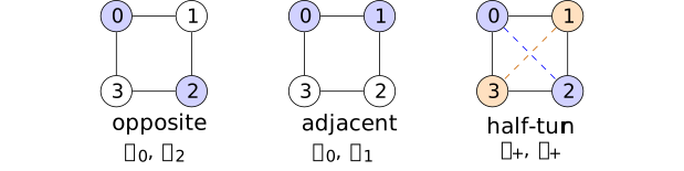
In the first two panels, filled vertices are retained coordinates. In the third, the paired colors and dashed diagonals indicate the normalized sums \(x_+=(\phi _0+\phi _2)/\sqrt 2\) and \(y_+=(\phi _1+\phi _3)/\sqrt 2\); the diagonals are pairing guides, not added graph edges. All three observations have rank two.
For \(R=\{0,2\}\), use the orthonormal retained basis \((\delta _0,\delta _2)\). Compressing \(G\) and inverting gives \[\begin {aligned} C_{\mathrm {opp}}&=\frac 1{15}\begin {pmatrix}7&2\\2&7\end {pmatrix},\\ S_{\mathrm {opp}}&=\frac 13\begin {pmatrix}7&-2\\-2&7\end {pmatrix}. \end {aligned}\] The sum and difference vectors have precision eigenvalues \(5/3,3\); their product is \(\det S_{\mathrm {opp}}=5\). This is the opposite-vertex marginal.
For \(R=\{0,1\}\), use \((\delta _0,\delta _1)\). The same operation yields \[\begin {aligned} C_{\mathrm {adj}}&=\frac 1{15}\begin {pmatrix}7&3\\3&7\end {pmatrix},\\ S_{\mathrm {adj}}&=\frac 18\begin {pmatrix}21&-9\\-9&21\end {pmatrix}. \end {aligned}\] Its sum and difference eigenvalues are \(3/2,15/4\), with \(\det S_{\mathrm {adj}}=45/8\). This recovers the fixed-label counterexample as a change of selector.
Finally let \(H_2\delta _i=\delta _{i+2}\) be the half-turn and \(P_+=(I+H_2)/2\). In the orthonormal basis \[v_0=(\delta _0+\delta _2)/\sqrt 2,\qquad v_1=(\delta _1+\delta _3)/\sqrt 2\] of its image, the positive sector has \[\begin {aligned} C_+&=\frac 15\begin {pmatrix}3&2\\2&3\end {pmatrix},\\ S_+&=\begin {pmatrix}3&-2\\-2&3\end {pmatrix}. \end {aligned}\] Indeed \(Qv_0=3v_0-2v_1\) and \(Qv_1=-2v_0+3v_1\), so this space is \(Q\)-invariant and the retained precision is the restriction. Its eigenvalues are \(1,5\), with determinant \(5\). The coordinates are normalized sums \((\phi _0+\phi _2)/\sqrt 2\), \((\phi _1+\phi _3)/\sqrt 2\), not the values of two retained vertices.
All three laws follow from the selected-law theorem with the displayed basis choices. Equal rank, or even the shared determinant \(5\) of the first and third examples, does not force equal retained spectra.
Example 9. Quaternion and coordinate selectors [fdip-005G]AGENTDRAFTED
- November 1, 2026
Example 9. Quaternion and coordinate selectors [fdip-005G]AGENTDRAFTED
- November 1, 2026
Let \(\Gamma =Q_8=\{\pm 1,\pm i,\pm j,\pm k\}\) and take the simple undirected Cayley graph with edges \(\{g,gs\}\), \(s\in \{\pm i,\pm j\}\), counted once each. Give each edge weight one, choose any orientation, and set \(m=1\). The two parts \[A=\{\pm 1,\pm k\},\qquad B=\{\pm i,\pm j\}\] give \(K_{4,4}\): every vertex in one part has the 4 distinct vertices of the other as its neighbors. In part order, \[L=\begin {pmatrix}4I_4&-J_4\\-J_4&4I_4\end {pmatrix}, \qquad Q=L+I_8,\] where \(J_4\) is the all-ones matrix. The two constant-on-part vectors give Laplacian eigenvalues \(0,8\); the two partwise zero-sum spaces give eigenvalue \(4\), of total multiplicity 6.
Left multiplication gives a signed graph action \(\rho \) on \(\mathbb R^{Q_8}\), independent of the arbitrary edge orientations. For the central involution \(z=-1\), put \[e_-=(1-[z])/2\in \mathbb R[Q_8],\qquad P_-=\rho (e_-)=(I-\rho (z))/2.\] Since \(z^2=1\) and \(z^{-1}=z\), this is a self-adjoint idempotent. Its image is the four-dimensional space of fields \(f(-g)=-f(g)\). The group-algebra decomposition \(\mathbb R[Q_8]\cong \mathbb R^4\times \mathbb H\) in Proposition [fgap-001B] sends \(e_-\) to \((0,1)\): each real character takes \(z\) to \(1\), while the quaternionic realization takes it to \(-1\). Thus this selector retains precisely the quaternion factor in the regular module, without assigning it a physical interpretation.
Proof.
- November 1, 2026
Proof.
- November 1, 2026
An odd field has zero sum on each of \(A,B\), since each part is a union of pairs \(\{g,-g\}\). Therefore \(J_4\) kills its restriction to either part, and the displayed Laplacian gives \(Lf=4f\). An orthonormal basis is \((\delta _g-\delta _{-g})/\sqrt 2\) for \(g=1,i,j,k\). Hence the selected precision is \[S_-=5I_4,\qquad C_-=I_4/5.\] Equivalently, the two neighbor contributions indexed by \(s,-s\) cancel on an odd field. The positive mass supplies the shift from \(4\) to \(5\).
Compare the coordinate selector on the subgroup \(R=\langle i\rangle =\{1,-1,i,-i\}\), which retains two vertices from each part. In the full graph, decompose fields into the two constant-on-part lines and the two partwise zero-sum spaces. On the normalized part constants, the precision and covariance are \[\begin {pmatrix}5&-4\\-4&5\end {pmatrix},\qquad \frac 19\begin {pmatrix}5&4\\4&5\end {pmatrix};\] on the zero-sum spaces the covariance is \(1/5\). It follows that full covariance entries are \(13/45\) on the diagonal, \(4/45\) between distinct vertices in the same part, and \(1/9\) between parts. For example the first entry is \((1-1/4)/5+(5/9)/4=13/45\).
In retained order \((1,-1,i,-i)\), compression therefore gives \[C_R=\frac 1{45}\begin {pmatrix} 13&4&5&5\\4&13&5&5\\5&5&13&4\\5&5&4&13 \end {pmatrix}.\] The two within-part difference vectors have covariance eigenvalue \((13-4)/45=1/5\). On normalized retained part constants the covariance block is \(\frac 1{45}\begin {pmatrix}17&10\\10&17\end {pmatrix}\), with eigenvalues \(3/5,7/45\). Inversion gives the retained precision spectrum \[\operatorname {spec}(S_R)=\{5/3,5,5,45/7\}.\] It differs from \(\{5,5,5,5\}\) for the quaternion selector despite equal rank and the same full background precision.
The chosen \(Q_8\) action is auxiliary data used to construct \(P_-\); it is not another slot of the selected tuple. Indeed the underlying graph has \(2(4!)^2=1152\) automorphisms: its connected bipartition is unique up to exchange, and every permutation within either part, as well as their exchange, preserves all edges. The selected-background groupoid remembers the graph and the resulting projector, not a named subgroup of this automorphism group. Remembering the action would require an enhanced tuple and arrows intertwining that action.
Proposition 10. Invariants of a selected background [fdip-005J]AGENTDRAFTED
- November 1, 2026
Proposition 10. Invariants of a selected background [fdip-005J]AGENTDRAFTED
- November 1, 2026
For a selected background, put \(X=\operatorname {im}P\). The following are invariants of its orthogonal comparison class:
- the spectrum of \(Q\), with multiplicities, and the rank of \(P\);
- the spectrum of \(S_P\), hence its determinant and trace;
- for each eigenvalue \(\lambda \) of \(Q\), the principal angles between \(X\) and \(E_\lambda =\ker (Q-\lambda I)\).
Here principal angles are defined by taking orthonormal inclusion matrices \(B_X,B_\lambda \) and the \(\min (\dim X,\dim E_\lambda )\) singular values of \(B_X^*B_\lambda \). These numbers lie in \([0,1]\); their arccosines, in increasing order, are the angles. This definition includes zero singular values and uses the entire eigenspace when \(\lambda \) is repeated. It is independent of the two orthonormal bases.
Proof.
- November 1, 2026
Proof.
- November 1, 2026
If \(Q'=OQO^{-1}\) and \(P'=OPO^{-1}\), then \(O(X)=X'\) and \(O(E_\lambda )=E'_\lambda \). Choosing the transported bases leaves \(B_X^*B_\lambda \) unchanged; changing either basis multiplies this matrix on the left or right by an orthogonal matrix, which does not change its singular values. These are at most one because both inclusions and orthogonal projections have operator norm at most one. Conjugation gives the spectrum of \(Q\) and rank of \(P\). The selected-law transport gives \(S_{P'}=(O|_X)S_P(O|_X)^{-1}\), proving the remaining claims.
These are consequently invariants of both graph groupoids \(\mathsf {Bg}\) and \(\mathsf {Bg}^{\pm }\). There is additional incidence information: the isomorphism class of the weighted incidence presentation with its selector, and the order of its finite automorphism group, are invariants in the chosen graph groupoid. Indeed, an arrow \(g:b\to b'\) induces the group isomorphism \(\alpha \mapsto g\alpha g^{-1}\) of automorphism groups. The directed and signed groups are different choices here; \(|\operatorname {Aut}_{\mathsf {Bg}}(b)|\) is not being asserted invariant under an arbitrary signed arrow.
The cospectral pair has an orthogonal comparison but no graph arrow. Thus even all the listed spectral and angle invariants cannot recover incidence. No completeness claim for invariants of the pair \((Q,P)\) under \(O(H)\) is made.
TauCeti's TauCeti.cosPrincipalAngles defines
the singular values of the overlap operator of two finite
orthonormal families as a nonincreasing sequence padded by zeros.
Taking its first \(\min (\dim X,\dim E_\lambda )\) values and then
arccosines gives the convention above. Its
TauCeti.cosPrincipalAngles_le_one supplies the
upper bound; the background-conjugacy and incidence claims are
the separate arguments here.
Theorem 11. Three inequivalent selectors and their observables [fdip-005K]AGENTDRAFTED
- November 1, 2026
Theorem 11. Three inequivalent selectors and their observables [fdip-005K]AGENTDRAFTED
- November 1, 2026
On the unit four-cycle with \(m=1\), the opposite, adjacent and positive half-turn selectors are pairwise inequivalent under the orthogonal comparison. Consequently no directed or signed graph arrow identifies any pair. Their retained precisions have the following invariants:
\[\begin {array}{c|c|c|c} \text {selector}&\operatorname {spec}S_P&\det S_P&\operatorname {tr}S_P\\\hline \text {opposite}&\{5/3,3\}&5&14/3\\ \text {adjacent}&\{3/2,15/4\}&45/8&21/4\\ \text {half-turn}&\{1,5\}&5&6. \end {array}\]
Proof.
- November 1, 2026
Proof.
- November 1, 2026
The three two-by-two precisions and their eigenvectors are computed in Example 8. Their distinct spectra separate them by the invariance proposition. Products and sums of the eigenvalues give the displayed determinants and traces.
The intrinsic squared-norm observable has expectation \[\mathbb E_{\mu _Q}\|P\phi \|^2 =\mathbb E_{\nu _b}\|x\|^2 =\operatorname {tr}_X C_P =\operatorname {tr}_H(PG).\] Indeed, in an orthonormal basis of \(X\) the squared norm is the sum of squares of coordinates, each with variance equal to the corresponding diagonal covariance entry. Since \(C_P=(PGP)|_X\) and \(P^2=P\), cyclicity of the finite-dimensional trace gives the last equality. In the same order as the table, \[\mathbb E\|P\phi \|^2=\frac {14}{15},\quad \frac {14}{15},\quad \frac 65.\] The reciprocal eigenvalues give these values. Thus neither \(\det S_P\) nor this covariance trace alone separates all three selectors. In particular the equal covariance traces of the first two do not mean equal precision traces.
For the two coordinate selectors, named coordinate observations also distinguish the laws. The full covariance in Example 8 gives \[\begin {aligned} \frac {\langle \phi _0\phi _2\rangle }{\langle \phi _0^2\rangle } &=\frac 27&&\text {(opposite)},\\ \frac {\langle \phi _0\phi _1\rangle }{\langle \phi _0^2\rangle } &=\frac 37&&\text {(adjacent)}. \end {aligned}\] The marginal expectation identity makes these the corresponding retained expectations. They refer to the stated vertex coordinates; unlike the spectrum and squared norm, such coordinate ratios are not invariants under arbitrary orthogonal changes of retained basis.
Corollary 12. The unselected graph does not determine the retained law [fdip-005L]AGENTDRAFTED
- November 1, 2026
Corollary 12. The unselected graph does not determine the retained law [fdip-005L]AGENTDRAFTED
- November 1, 2026
On selected backgrounds, the retained-precision spectrum does not factor through the isomorphism class of the unselected weighted incidence data \((\Pi ,w,m)\). In particular, that unselected class does not determine the retained Gaussian law up to a precision-intertwining isometry. This holds for either the directed or the signed graph groupoid.
Proof.
- November 1, 2026
Proof.
- November 1, 2026
Take isomorphism classes in the chosen groupoid and apply the forgetful map that removes \(P\). The retained spectrum is well-defined on these classes by Proposition 10. The three four-cycle selections have exactly the same incidence, weights and mass, so they belong to one fiber of the forgetful map, but their retained spectra differ. The fiber-constancy criterion therefore rules out a factorization through the unselected class. An isometric intertwiner of retained precisions would preserve their spectra, so it cannot identify these retained laws.
This obstruction concerns forgetting the selector, not a failure of the selected-law formula: \((\Pi ,w,m,P)\) does determine \(\nu _b\). In the other direction, the weighted-cycle comparison fixes the coordinate selector and mass while changing the weights; its retained covariance changes. Together the examples show why both the weighted incidence data and the selector must be retained to specify the observed law. They supply no physical rule for how either datum varies.
Theorem 13. When a marginal precision is a restriction [fdip-005M]AGENTDRAFTED
- November 1, 2026
Theorem 13. When a marginal precision is a restriction [fdip-005M]AGENTDRAFTED
- November 1, 2026
Let \(Q>0\) be self-adjoint on a finite-dimensional real Euclidean space \(H\) and let \(P\) be an orthogonal projector. Assume its image \(X\) and kernel \(Y\) are nonzero. In \(H=X\oplus Y\), write \[Q=\begin {pmatrix}A&K\\K^*&D\end {pmatrix},\qquad D>0.\] The selected precision obeys \[S_P=A-KD^{-1}K^*\preceq A.\] Here \(A=PQ|_X\) is the compression, and \(T\preceq A\) means that \(\langle x,(A-T)x\rangle \ge 0\) for every \(x\in X\). The following conditions are equivalent: \[\begin {aligned} S_P=A&\quad \Longleftrightarrow \quad K=0\\ &\quad \Longleftrightarrow \quad QX\subseteq X \quad \Longleftrightarrow \quad PQ=QP. \end {aligned}\] In this case \(A=Q|_X\); call the selector restricting. Otherwise it induces a different precision through elimination of the complement.
Proof.
- November 1, 2026
Proof.
- November 1, 2026
The Schur formula is proved in Theorem 2. Its difference from the compression satisfies \[\langle x,(A-S_P)x\rangle =\|D^{-1/2}K^*x\|^2\ge 0.\] It vanishes for all \(x\) exactly when \(K^*=0\), since \(D^{-1/2}\) is invertible. The \(Y\)-component of \(Q(x,0)\) is \(K^*x\), so the same condition is \(QX\subseteq X\). Self-adjointness then makes \(Y=X^\perp \) invariant as well: \(\langle Qy,x\rangle =\langle y,Qx\rangle =0\). The resulting block diagonal matrix commutes with \(P\); conversely \(PQ=QP\) carries its image to itself.
When \(K\ne 0\), the positive semidefinite difference \(A-S_P\) is nonzero, so the quadratic form decreases in some direction. It need not be positive definite: some directions may have zero loss. The assertion is a Loewner inequality with the stated equality criterion, not a strict inequality in every direction.
For a positive-weight graph and a coordinate selector \(P_R\), \(K\) consists of the entries of \(Q\) between \(R\) and its complement. For distinct vertices these are minus the sum of weights of edges joining them; orientation does not affect the sum. All summands are positive. Hence \(K=0\) exactly when no edge joins \(R\) to its complement. In a connected graph every nonempty proper coordinate selector therefore induces a different precision. In particular, the retained vertices in cycle decimation are stable under the retained cyclic action, but this symmetry does not make their span \(Q\)-invariant.
In orthonormal coordinates, Mathlib's
Matrix.PosDef.inv gives positivity of \(D^{-1}\).
The congruence lemma
Matrix.PosSemidef.mul_mul_conjTranspose_same,
with its positive semidefinite matrix set to \(D^{-1}\) and its
rectangular matrix set to \(K\), gives \(KD^{-1}K^*\succeq 0\).
These declarations support the positivity steps. The equality
criterion, subspace equivalences and graph specialization are
proved above.
Corollary 14. Which symmetry selectors restrict [fdip-005N]AGENTDRAFTED
- November 1, 2026
Corollary 14. Which symmetry selectors restrict [fdip-005N]AGENTDRAFTED
- November 1, 2026
Let a finite group \(\Gamma \) act orthogonally on a finite-dimensional real Euclidean space \(H\), and let \(Q>0\) be self-adjoint and \(\Gamma \)-equivariant. Two constructions of symmetry selectors have different criteria.
- For a self-adjoint idempotent \(e\in \mathbb R[\Gamma ]\), the selector \(P=\rho (e)\) restricts whenever its rank is nonzero and proper. Its image need not be a \(\Gamma \)-subrepresentation.
- A nonzero proper \(\Gamma \)-subrepresentation \(X\) restricts precisely when its multiplicity subspace in every real isotypic block is invariant under the corresponding Hermitian precision matrix \(Q_\Xi \).
Here is the precise multiplicity convention. Use the real commutant and the right-scalar column coordinates. For \(D_\Xi =\operatorname {End}_\Gamma (W_\Xi )\) and \(r_\Xi =\dim _{D_\Xi }W_\Xi \), represent \(H_\Xi \) by \(r_\Xi \) columns in \(D_\Xi ^{m_\Xi }\); matrices act on each column by left multiplication. There is a right \(D_\Xi \)-subspace \(U_\Xi \subseteq D_\Xi ^{m_\Xi }\) such that \[X\cap H_\Xi \cong \{(z_1,\ldots ,z_{r_\Xi }):z_a\in U_\Xi \}.\] The criterion is \[Q_\Xi U_\Xi \subseteq U_\Xi \qquad \text {for every }\Xi .\] Equivalently, each \(U_\Xi \) has a \(D_\Xi \)-basis of \(Q_\Xi \)-eigenvectors. Repeated eigenvalues allow proper subspaces of an eigenspace; whole eigenspaces need not be selected.
Proof.
- November 1, 2026
Proof.
- November 1, 2026
Equivariance makes \(Q\) commute with every \(\rho (g)\), hence with \(\rho (e)\). The restriction criterion proves the first assertion. Centrality is not needed for this commutation; it would additionally make \(\rho (e)\) commute with the group action.
For a subrepresentation \(X\), both \(X\) and \(X^\perp \) are \(\Gamma \)-stable, so its orthogonal projector belongs to the commutant. By Theorem [fdip-004Z] it is represented by Hermitian idempotents \(p_\Xi \in M_{m_\Xi }(D_\Xi )\). In the stated column coordinates its image has exactly the displayed form with \(U_\Xi =\operatorname {im}p_\Xi \). Conversely a right \(D_\Xi \)-subspace has an orthogonal projector commuting with right scalar multiplication: its real orthogonal complement is right-scalar stable, since multiplication by each unit scalar is orthogonal and preserves the subspace. Thus that projector is a matrix over \(D_\Xi \); the commutant identification gives the corresponding subrepresentation.
The matrix \(Q_\Xi \) acts on every column, so \(QX\subseteq X\) is exactly the displayed invariance condition. If it holds, self-adjointness preserves the orthogonal complement too. The Hermitian spectral argument of Corollary [fdip-0050] applies to the restriction on \(U_\Xi \): a real eigenvector generates a right \(D_\Xi \)-line of eigenvectors, its orthogonal complement is invariant, and induction gives a \(D_\Xi \)-orthonormal eigenbasis. Conversely a span of eigenvectors is invariant, since their eigenvalues are real and the matrix is right-linear. Apply Theorem 13 to finish.
In a multiplicity-free representation every \(m_\Xi =1\), and a right \(D_\Xi \)-subspace of \(D_\Xi \) is either zero or all of it. Thus every nonzero proper subrepresentation restricts. At higher multiplicity, group stability alone does not suffice, as the prism line shows.
Example 15. A stable prism line and a partial eigenspace [fdip-005O]AGENTDRAFTED
- November 1, 2026
Example 15. A stable prism line and a partial eigenspace [fdip-005O]AGENTDRAFTED
- November 1, 2026
In the twisted prism, let \(e_u\) and \(e_l\) be the normalized constant vectors on the upper and lower triangles. The group \(\Gamma =C_3\) fixes each, and its trivial isotypic block has multiplicity two. In this orthonormal basis the precision and covariance are \[\begin {aligned} Q_{\mathrm {triv}} &=\begin {pmatrix}5/2&-3/2\\-3/2&5/2\end {pmatrix},\\ Q_{\mathrm {triv}}^{-1} &=\begin {pmatrix}5/8&3/8\\3/8&5/8\end {pmatrix}. \end {aligned}\] Their product is the identity; the determinant of the first is \(4\). The other isotypic block is orthogonal and uncoupled.
Select \(X=\mathbb R e_u\), the line of fields constant on the upper triangle and zero on the lower one. This line is \(\Gamma \)-stable, but \(Qe_u=(5/2)e_u-(3/2)e_l\notin X\). Its compressed covariance is \(5/8\), so \[S_P=\frac 85,\qquad PQ|_X=\frac 52.\] Equivalently, eliminating the lower constant line gives \[\frac 52-\frac {(3/2)^2}{5/2}=\frac 85.\] Thus this subrepresentation induces a different precision. By contrast, the lines spanned by \(e_u+e_l\) and \(e_u-e_l\) have precision eigenvalues \(1\) and \(4\), respectively. Their orthogonal selectors restrict, with retained precisions \(1\) and \(4\). This directly verifies the multiplicity-subspace criterion.
The word eigenvectors in that criterion cannot be replaced by whole eigenspaces. Let the trivial group act on the unit four-cycle. The precision has eigenvalue \(3\) on the two-dimensional space spanned by \[v=(1,0,-1,0),\qquad w=(0,1,0,-1).\] Direct multiplication gives \(Qv=3v\) and \(Qw=3w\). The selector onto \(\mathbb R v\) is proper within this eigenspace and restricts, with \(S_P=3\) in the unit coordinate \(v/\sqrt 2\). Every subspace is stable under the trivial group, but only \(Q\)-invariant ones meet the restriction criterion.
Remark 16. Isotropy pieces of the background parameter set [fdip-005P]AGENTDRAFTED
- November 1, 2026
Remark 16. Isotropy pieces of the background parameter set [fdip-005P]AGENTDRAFTED
- November 1, 2026
For a fixed incidence presentation \(\Pi \), let \(K_\Pi \) be its finite group of signed endpoint automorphisms, acting on the parameter set \(\mathcal B_\Pi \). The isotropy group at \(b\) is \((K_\Pi )_b=\{g:g b=b\}\). Partition \(\mathcal B_\Pi \) by the conjugacy class in \(K_\Pi \) of this stabilizer. These are its isotropy pieces. If \(b'=g b\), then \((K_\Pi )_{b'}=g(K_\Pi )_b g^{-1}\), so an orbit stays inside one piece. Between different presentations, graph arrows still identify the automorphism groups, without placing all of them inside one common acting group.
Write \(b_{a,b}\) for the alternating four-cycle with positive weights \((a,b,a,b)\), fixed \(m>0\), and retained pair \(\{0,2\}\). The signed stabilizer calculation gives \[\operatorname {Aut}_{\mathsf {Bg}^{\pm }}(b_{a,b}) \cong \begin {cases} C_2&a\ne b,\\ C_2\times C_2&a=b. \end {cases}\] This is a change of isotropy at equal weights. In the directed groupoid the uniformly oriented unit cycle admits only rotations; preserving \(\{0,2\}\) leaves the identity and half-turn, so its stabilizer is \(C_2\). Reflections belong to the larger signed convention.
The orthogonal stabilizers of the same pair \((Q,P_R)\) are \((C_2)^2\) and \((C_2)^3\), as proved in Proposition 6. They describe a different comparison and do not define the graph isotropy pieces above. Here strata can mean only this set-level partition by isotropy type. No smooth stratification, analytic singularity or physical phase transition follows from it. Those further interpretations require additional structure and arguments.