Enriched backgrounds and comparison [fdip-001E]
✍️sourceAGENTDRAFTED
- October 20, 2026
Enriched backgrounds and comparison [fdip-001E]
✍️sourceAGENTDRAFTED
- October 20, 2026
Which data must a comparison preserve for observables to survive? The finite background, its reference pairing and retained split already distinguish a relabeling from an arbitrary field map. The cycle trace ratio gives an observable with which to test a proposed comparison.
The enriched groupoid records allowed arrows and the data they preserve. Scalar invariants descend along those arrows without classifying all backgrounds. Quadratic isometry can forget the reference pairing or retained projection even while transporting a positive Gaussian law. Its Clifford functoriality therefore need not retain all the information required for these observables.
Example 1. The groupoid of enriched four-cycle backgrounds [fdip-000X]AGENTDRAFTED
- October 18, 2026
Example 1. The groupoid of enriched four-cycle backgrounds [fdip-000X]AGENTDRAFTED
- October 18, 2026
A classification of Gaussian backgrounds must retain the maps that transport their observables. Consider the alternating four-cycle with vertices \(V=\mathbb Z/4\mathbb Z\), forward edges \(e_i:i\to i+1\), and weights \((a,b,a,b)\), where \(a,b>0\). Choose \(m>0\) and one of \(R_0=\{0,2\}\), \(R_1=\{1,3\}\) as retained vertices. Write \(x=(a,b,m,R_j)\) and let \(X\) be the set of all these tuples. The tuple specifies a finite Gaussian background, together with its named half-turn.
More explicitly, retain the carrier, counting reference pairing, weight matrix \(W_x=\operatorname {diag}(a,b,a,b)\), and \[L_x=B^TW_xB,\qquad Q_x=L_x+m^2I.\] Here \((B\phi )_i=\phi _{i+1}-\phi _i\). For \(\phi \ne 0\), \[\begin {aligned} \phi ^TQ_x\phi &=\sum _iw_i(\phi _{i+1}-\phi _i)^2\\ &\quad +m^2\|\phi \|^2>0. \end {aligned}\] The normalized Gaussian \(\mu _{Q_x}\) is determined by this precision and coordinate Lebesgue measure. Also retain the measurable coordinate projection \(\pi _{R_j}:\mathbb R^V\to \mathbb R^{R_j}\) and the named action \(\rho (h)\delta _i=\delta _{i+2}\) of \(C_2=\{1,h\}\). The vertex basis \(\delta _i(v)=\mathbf 1_{v=i}\) is distinct from the edges \(e_i\) and the spectral vectors \(u_a\). These structures are specified or determined, rather than additional freely variable coordinates of \(X\).
Allow rotations and reflections of the underlying cycle. Put \[D_4=\langle r,s\mid r^4=s^2=1,\ srs=r^{-1}\rangle ,\] where \(r(i)=i+1\) and \(s(i)=-i\). A reflection reverses the forward orientation. Thus these arrows use the signed endpoint convention and extend the earlier strictly directed exact relabelings. For \(g=r^ks^\varepsilon \), with \(k\in \mathbb Z/4\) and \(\varepsilon \in \{0,1\}\), set \[\begin {aligned} g(i)&=k+(-1)^\varepsilon i,\\ P_g\delta _i&=\delta _{g(i)},\\ \tau _g(i)&=\begin {cases}k+i&\varepsilon =0,\\k-i-1&\varepsilon =1,\end {cases}\\ U_g\eta _i&=(-1)^\varepsilon \eta _{\tau _g(i)}. \end {aligned}\] Here \(\eta _i\) is the edge-field coordinate basis. All indices are modulo \(4\). The 8 vertex maps are distinct because their values at \(0,1\) determine \(k,\varepsilon \).
The edge indexed by \(\tau _g(i)\) has endpoints \(g(i),g(i+1)\), in forward order for a rotation and reverse order for a reflection. Consequently, for every field \(\phi \), \[\begin {aligned} (BP_g\phi )_{\tau _g(i)}&=(-1)^\varepsilon (B\phi )_i,\\ BP_g&=U_gB. \end {aligned}\] If \(k'\) denotes a second group element, endpoint transport and multiplication of the orientation signs give \[P_{k'g}=P_{k'}P_g,\qquad U_{k'g}=U_{k'}U_g.\] For an explicit group-law check, composition of \((k,\varepsilon )\) followed by \((\ell ,\eta )\) gives \[\begin {aligned} (\ell ,\eta )(k,\varepsilon ) &=(\ell +(-1)^\eta k,\eta +\varepsilon ). \end {aligned}\] The second coordinate is taken modulo two. Both coordinate maps are orthogonal, and their inverses are indexed by \(g^{-1}\).
Transport weights by \(W_{gx}=U_gW_xU_g^T\) and the retained set by \(R\mapsto gR\). The signs cancel in the diagonal weight matrix. The weights swap exactly when \(k+\varepsilon \) is odd, while \(R_j\mapsto R_{j+k\bmod 2}\). In particular, \[\begin {aligned} r(a,b,m,R_j)&=(b,a,m,R_{j+1}),\\ s(a,b,m,R_j)&=(b,a,m,R_j). \end {aligned}\] The family is closed under these maps, with mass unchanged. Using \(BP_g^T=U_g^TB\) gives \[\begin {aligned} L_{gx}&=B^TU_gW_xU_g^TB=P_gL_xP_g^T,\\ Q_{gx}&=P_gQ_xP_g^T. \end {aligned}\] Moreover \(g(i+2)=g(i)+2\), so every arrow commutes with the same named half-turn: \(P_g\rho (h)=\rho (h)P_g\).
Form the action groupoid \(D_4\ltimes X\) by setting \[\operatorname {Hom}(x,y)=\{g\in D_4:g x=y\}.\] The group element remains part of an arrow. Compose \(g:x\to y\) and \(k:y\to z\) as \(kg:x\to z\); the action law gives its target. The identity is \(1:x\to x\), the inverse is \(g^{-1}:gx\to x\), and the two inverse identities and associativity follow from the group laws. Thus every arrow is invertible, as in [stacks2017stacks, Definition 4.2.5], Tag 0018. The source, target and composition follow the set-level pattern in [stacks2017stacks, Lemma 78.15.1], Tag 0444; that lemma is stated for algebraic spaces, whereas the axioms here were checked directly for sets. \(X\) is infinite, but each orbit and its restricted groupoid is finite.
The stabilizer of the weights at \(a\ne b\) is \(\{1,r^2,rs,r^3s\}\cong C_2\times C_2\); preserving weights requires \(k+\varepsilon \) even. The stabilizer of either retained partition is \(\{1,r^2,s,r^2s\}\cong C_2\times C_2\), since preserving the partition requires \(k\) even. Intersecting these conditions gives the following automorphism groups. When \(a\ne b\), \[\operatorname {Aut}(x)=\{1,r^2\}\cong C_2.\] When \(a=b\), \[\begin {aligned} \operatorname {Aut}(x)&=\{1,r^2,s,r^2s\}\\ &\cong C_2\times C_2. \end {aligned}\] At equal weights the first condition disappears. In each four-element subgroup the two indicated generators are distinct commuting involutions. No further condition comes from the named half-turn, which commutes with all 8 elements. The kernel \(\{1,r^2\}\) of the parameter action is retained as distinct arrows: \(P_{r^2}\delta _0=\delta _2\ne \delta _0\).
For unequal weights the orbit consists of both weight orders and both partitions, at fixed mass. Write \(x_j=(a,b,m,R_j)\) and \(y_j=(b,a,m,R_j)\). The drawing shows selected generator arrows; it does not draw all arrows or isotropy loops.
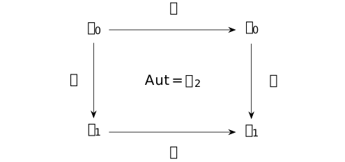
At \(a=b\), put \(z_j=(a,a,m,R_j)\). There are two objects, each with automorphism group \(C_2\times C_2\):

The generators \(s,r\) reach every displayed object; there are exactly 4 objects when \(a\ne b\) and two when \(a=b\). It follows in both directions that the coarse isomorphism classes are \((m,\{a,b\})\). The coarse orbit set forgets the isotropy just computed, as in Example [fgap-000P]. On the strict slice \((1,t,m,R_0)\), isomorphism requires the same mass and \(\{1,t\}=\{1,t'\}\), whose products give \(t=t'\). Thus reciprocal parameters are not identified there unless \(t=1\). This is a set-level groupoid, within the boundary before stacks.
Mathlib's CategoryTheory.ActionCategory constructs
the generic action category; a group action makes it a groupoid.
CategoryTheory.ActionCategory.stabilizerIsoEnd
identifies the stabilizer monoid with endomorphisms, which are invertible
in the group case. MulAction.orbitRel and
MulAction.stabilizer provide the generic coarse relation
and subgroup. DihedralGroup.card gives 8 elements
at \(n=4\), and DihedralGroup.center_eq_closure_of_even_ne_two
gives the central half-turn. In its constructor convention our
\(r^ks\) corresponds to \(\texttt {sr}(-k)\), while \(r^k\)
corresponds to \(\texttt {r}(k)\). These declarations support the
group constructions; the particular parameter action, signed incidence
and stabilizer intersections are the calculations above.
Proposition 2. Scalar descent and transport of Gaussian observables [fdip-000Y]AGENTDRAFTED
- October 18, 2026
Proposition 2. Scalar descent and transport of Gaussian observables [fdip-000Y]AGENTDRAFTED
- October 18, 2026
On the enriched four-cycle groupoid, the trace ratio, with the cycle values, is a scalar on isomorphism classes, while covariance and effective precision are transported operators on their specified field spaces. For \(x=(a,b,m,R)\) write \(C_x=Q_x^{-1}\). If \(g:x\to y\), then \[\begin {aligned} C_y&=P_gC_xP_g^T,\\ (P_g)_*\mu _{Q_x}&=\mu _{Q_y},\\ \langle F\rangle _{Q_y}&=\langle F\circ P_g\rangle _{Q_x}. \end {aligned}\] The last identity holds for Borel \(F\in L^1(\mu _{Q_y})\); integrability is equivalent to that of \(F\circ P_g\) in the source law. These statements use the inverse-precision covariance and Gaussian transport, including their normalization.
Proof.
- October 18, 2026
Proof.
- October 18, 2026
The groupoid construction proves \(Q_y=P_gQ_xP_g^T\) and \(P_g^{-1}=P_g^T\). Inverting gives the covariance equation. The normalized density in dimension \(4\) is \[d\mu _Q(\phi )=\frac {\sqrt {\det Q}}{(2\pi )^2} e^{-\phi ^TQ\phi /2}\,d\phi .\] Set \(\psi =P_g\phi \). The absolute Jacobian is one. The exponent is now \(-\psi ^TQ_y\psi /2\). Also \(\det Q_y=\det Q_x\), proving the pushforward identity. Apply the same substitution to \(|F|\) first, then to the positive and negative parts when finite, to prove the expectation statement. Transport composes because \(P_{kg}=P_kP_g\).
Transport does not imply equality of labeled arrays. At \((a,b,m)=(1,2,1)\), the spectral covariance formula gives \[\begin {aligned} (C_x)_{01} &=\tfrac 14(1-\tfrac 13+\tfrac 15-\tfrac 17)\\ &=\tfrac {19}{105},\\ (P_rC_xP_r^T)_{01} &=\tfrac 14(1+\tfrac 13-\tfrac 15-\tfrac 17)\\ &=\tfrac {26}{105}. \end {aligned}\] The second entry is the old \((3,0)\) entry. The observable's coordinate labels must move with the field to preserve its expectation.
Let \(D=V\setminus R\). In retained/eliminated coordinates write \[\begin {aligned} Q_x&=\begin {pmatrix}A&H\\H^T&C_D\end {pmatrix},\\ S_R(x)&=A-HC_D^{-1}H^T. \end {aligned}\] This Schur complement is the positive precision of the marginal. The restrictions of \(g\) give permutation isometries \(P_R:\mathbb R^R\to \mathbb R^{gR}\) and \(P_D:\mathbb R^D\to \mathbb R^{gD}\). Then \[\begin {aligned} S_{gR}(y)&=P_RS_R(x)P_R^T,\\ S_{gR}(y)^{-1}&=P_RS_R(x)^{-1}P_R^T,\\ \pi _{gR}P_g&=P_R\pi _R. \end {aligned}\] Thus the marginal laws are compatible on the changing retained spaces.
Proof.
- October 18, 2026
Proof.
- October 18, 2026
The transformed blocks are \[\begin {aligned} A'&=P_RAP_R^T,\\ H'&=P_RHP_D^T,\\ C_D'&=P_DC_DP_D^T. \end {aligned}\] Substitution, using \(P_D^TP_D=I\), gives \[\begin {aligned} S_{gR}(y)&=A'-H'(C_D')^{-1}(H')^T\\ &=P_R(A-HC_D^{-1}H^T)P_R^T. \end {aligned}\] Inversion proves the covariance equation. The projection identity holds on each vertex coordinate vector. Consequently \[\begin {aligned} (P_R)_*\mu _{S_R(x)} &=(P_R\pi _R)_*\mu _{Q_x}\\ &=(\pi _{gR}P_g)_*\mu _{Q_x}\\ &=(\pi _{gR})_*\mu _{Q_y} =\mu _{S_{gR}(y)}. \end {aligned}\] Restrictions of composable permutations compose on these spaces, so the identities are compatible with composition.
For either opposite pair in ascending coordinate order, put \(d=a+b+m^2\). Direct block multiplication gives \[\begin {aligned} A=C_D&=dI_2,\\ H&=-\begin {pmatrix}a&b\\b&a\end {pmatrix},\\ S_R(x)&=\begin {pmatrix}\alpha &-\beta \\-\beta &\alpha \end {pmatrix},\\ \alpha &=d-\frac {a^2+b^2}{d},\\ \beta &=\frac {2ab}{d}. \end {aligned}\] This particular two-by-two array is unchanged by swapping weights or retained coordinates. That special equality does not make general operator assignments scalar invariants; the full covariance entries above already differ.
For the nonzero positive semidefinite \(L_x\), define \[\mathcal R(x)=\frac {\operatorname {tr}(L_x^2)} {\bigl (\operatorname {tr}L_x\bigr )^2}.\] Then \(\mathcal R(gx)=\mathcal R(x)\), and \[\mathcal R(a,b)=\frac {a^2+ab+b^2}{2(a+b)^2}.\] This scalar descends to the coarse orbit set but does not classify the enriched objects.
Proof.
- October 18, 2026
Proof.
- October 18, 2026
Trace cyclicity gives \(\operatorname {tr}(P_gMP_g^T)=\operatorname {tr}M\). Also \(L_{gx}^2=P_gL_x^2P_g^T\); hence both traces are preserved. For the explicit value, the 4 orthonormal vectors \(u_0,u_1,u_2,u_3\) from Example [fdip-0037] remain eigenvectors after replacing weights \((1,t)\) by \((a,b)\), with eigenvalues \(0,2a,2b,2a+2b\). Substituting the alternating entries of \(L_x\) verifies each eigenvector equation. Therefore \[\begin {aligned} \operatorname {tr}L_x&=4(a+b)>0,\\ \operatorname {tr}(L_x^2)&=8(a^2+ab+b^2). \end {aligned}\] These spectral trace identities use [boyd2004convex, Appendix A.5.2, pp. 646-647]. The positive denominator justifies the division. In particular \[\begin {aligned} \mathcal R(1,1)&=\frac 38,\\ \mathcal R(1,2)&=\frac 7{18},\\ \frac 7{18}-\frac 38&=\frac 1{72}. \end {aligned}\] The ratio ignores \(m\), so backgrounds of different masses have the same value. It also satisfies \(\mathcal R(1,t)=\mathcal R(1,1/t)\), although the strict slice objects are inequivalent for \(t\ne 1\) by Example 1.
Now forget mass, state and partition and admit positive scaling of the Laplacian, as in the broader comparison: \[L'=cP_gLP_g^T,\qquad c>0.\] The numerator of \(\mathcal R\) gains \(c^2\), while its denominator gains the same factor. Thus the ratio is invariant under this different relation. A weight-swapping relabeling followed by \(c=1/t\) sends \(L(1,t)\) to \(L(1,1/t)\). Reciprocal parameters are identified in this reduced problem only; no scale arrow has been added to the original Gaussian groupoid. At fixed mass, \(cL+m^2I\ne cQ\) for \(c\ne 1\). If one instead rescales the entire precision to \(cQ\), then \[\begin {aligned} (cQ)^{-1}&=c^{-1}Q^{-1},\\ cA-(cH)(cC_D)^{-1}(cH)^T&=cS_R. \end {aligned}\] Raw covariance and effective precision therefore are not scale invariants. Any normalized operator ratio would need its own definition and scaling proof.
Mathlib's Matrix.trace_units_conj and
Matrix.trace_smul support the trace conjugacy and scaling
identities. Matrix.reindexLinearEquiv and
Matrix.reindexRingEquiv supply coordinate infrastructure.
TauCeti's
TauCeti.Probability.map_affine_multivariateGaussian
allows positive semidefinite covariance and an arbitrary rectangular
linear map. Set its mean and translation to zero, its covariance
to \(Q_x^{-1}\), and its linear map to \(P_g\) or \(\pi _R\).
The precision-density identification and the Schur and groupoid
computations above remain separate obligations.
Example 3. Quadratic isometry forgets the reference pairing and projection [fdip-000Z]AGENTDRAFTED
- October 18, 2026
Example 3. Quadratic isometry forgets the reference pairing and projection [fdip-000Z]AGENTDRAFTED
- October 18, 2026
The enriched classification changes if one keeps only a positive quadratic form and permits every linear isometry. Any two positive symmetric matrices \(Q_1,Q_2\) of the same size define isometric quadratic spaces, even when their counting-relative spectra and retained observables differ.
[boyd2004convex, Appendix A.5.2, pp. 646-647] gives the symmetric spectral decomposition and positive square root used below to construct the isometry.
For \(Q=O\operatorname {diag}(\lambda _i)O^T\), with \(O\) orthogonal and every \(\lambda _i>0\), define \[\begin {aligned} Q^{1/2}&=O\operatorname {diag}(\sqrt {\lambda _i})O^T,\\ A=Q^{-1/2}&=O\operatorname {diag}(\lambda _i^{-1/2})O^T. \end {aligned}\] Direct multiplication gives \(A^TQA=I\). More generally, \[\begin {aligned} T&=Q_2^{-1/2}Q_1^{1/2},\\ T^TQ_2T &=Q_1^{1/2}Q_2^{-1/2}Q_2Q_2^{-1/2}Q_1^{1/2}\\ &=Q_1. \end {aligned}\] The map \(T\) is invertible. This calculation does not require \(Q_1Q_2=Q_2Q_1\). Thus positive quadratic forms have one linear-isometry class in each fixed dimension.
The reference pairing changes under the same substitution \(\phi =Az\): its matrix becomes \[H'=A^TIA=Q^{-1},\] while the action form has matrix \(I\). If that transported pairing is retained, its relative operator is \((H')^{-1}I=Q\), preserving the original spectrum. In general simultaneous transport of a positive reference pairing \(H\) and an action form \(Q\) gives \[\begin {aligned} H'&=A^THA,\qquad Q'=A^TQA,\\ (H')^{-1}Q'&=A^{-1}(H^{-1}Q)A. \end {aligned}\] Similarity preserves the spectrum. Replacing \(H'\) by \(I\) after normalizing \(Q\) discards this data; it is not simultaneous transport of the pair.
For the four-cycle with \(a=m=1\), compare \(b=1\) and \(b=2\). The spectral calculation gives respectively \[\begin {aligned} \operatorname {spec}(Q_1)&=\{1,3,3,5\},\\ \operatorname {spec}(Q_2)&=\{1,3,5,7\}. \end {aligned}\] These forms are linearly isometric by \(T\), but cannot be conjugate by a counting-orthogonal map, since their spectra differ. In particular they are not compatible relabelings. Their trace ratios also differ by \(1/72\).
The same isometry gives a concrete obstruction to the retained projection, even though it preserves the named half-turn. In the common orthonormal spectral basis \(u_0,u_1,u_2,u_3\), the matrix of \(T\) is \[\operatorname {diag}\bigl (1,1,\sqrt {3/5},\sqrt {5/7}\bigr ).\] The half-turn is diagonal in this basis as well, so \(T\rho (h)=\rho (h)T\). Returning to vertex coordinates gives \[T_{01}=\frac {\sqrt {3/5}-\sqrt {5/7}}4\ne 0,\] because \(3/5\ne 5/7\). For \(R=R_0\), one has \(\pi _R\delta _1=0\), whereas the zeroth component of \(\pi _RT\delta _1\) is nonzero. Hence no linear map \(T_R\) can satisfy \(\pi _RT=T_R\pi _R\). Also \(T^TT\) has eigenvalues \(1,1,3/5,5/7\), so \(T\) fails to preserve the counting pairing. These are separate failures of the enriched-arrow conditions.
A Jacobian magnitude different from one does not obstruct normalized Gaussian transport. If \(T^TQ_2T=Q_1\), then \[\det Q_1=(\det T)^2\det Q_2.\] For \(y=T\phi \), the exponent in the normalized density becomes \(-y^TQ_2y/2\); its coefficient after the reference change of variables is \[\frac {\sqrt {\det Q_1}}{(2\pi )^{n/2}|\det T|} =\frac {\sqrt {\det Q_2}}{(2\pi )^{n/2}}.\] Therefore \(T_*\mu _{Q_1}=\mu _{Q_2}\). Equivalently, \(Q_2^{-1}=TQ_1^{-1}T^T\) is the covariance transport law. For \(A=Q^{-1/2}\), the Jacobian magnitude \(|\det A|=(\det Q)^{-1/2}\) is exactly absorbed by normalization, even when it differs from one. The loss is the discarded pairing, carrier and retained projection, not a failure of normalized probability transport.
TauCeti's
Matrix.PosDef.exists_generalLinearGroup_mul_transpose_eq
provides an invertible factor \(C\) with \(Q=CC^T\) for a real
positive-definite matrix on a finite index set. For a bare witness
of that conclusion the normalizer is \(C^{-T}\), since
\[(C^{-T})^TQ C^{-T}=C^{-1}CC^TC^{-T}=I.\]
The theorem's proof chooses the symmetric positive square root,
but its existential conclusion does not assert symmetry of \(C\).
One therefore cannot infer that \(C^{-1}\) is the normalizer
from the factorization alone. Its separate
TauCeti.Probability.map_affine_multivariateGaussian
supports Gaussian transport in covariance parameters, after the
precision-density identification. Neither declaration supplies the
enriched classification or projection obstruction.
By Clifford functoriality, an isometry of these configuration forms also induces an algebra isomorphism. Since the positive forms already lie in one isometry class, keeping only the abstract quadratic space, or its isometry-functorial Clifford algebra, cannot recover the discarded reference pairing, carrier and projection. This argument does not infer a quadratic isometry from an arbitrary Clifford-algebra isomorphism. Retaining the enriched objects and their specified relabeling arrows prevents the demonstrated collapse; it supplies no continuum or physical selection map.