Arithmetic families [fdip-001D]
✍️sourceAGENTDRAFTED
- October 20, 2026
Arithmetic families [fdip-001D]
✍️sourceAGENTDRAFTED
- October 20, 2026
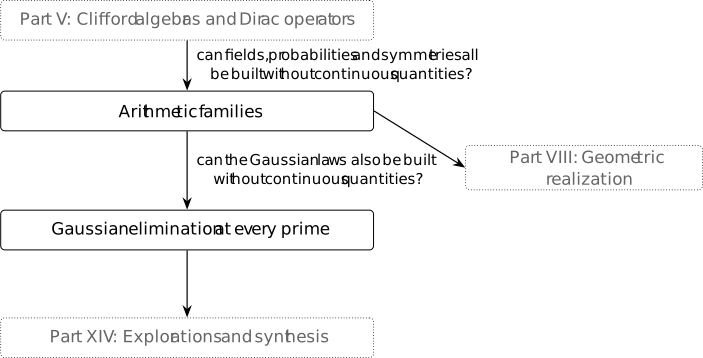
Which constructions survive if field values use finite arithmetic instead of the real numbers? For each prime \(p\), the finite field \(\mathbb F_p\) gives such a value system. Comparing it with a real model requires a specified arithmetic family and control of denominators. The four-cycle coefficients give an arithmetic family over \(\mathbb Z[1/2,t]\). Scalar extension organizes its Clifford algebras, while the form, elimination map and observable ratio each impose their own domain. Bad fibers distinguish those domains concretely. This base excludes characteristic two, where the earlier half-turn example shows how an algebra can survive while its sector decomposition changes.
The rational comparison uses Gaussian elimination and the reference pairing and trace conventions. It distinguishes the information in a quadratic center character from the independently defined trace observable. These arithmetic families also supply the fiber-constancy criterion used by the realization comparison.
With rational positive-definite precision in counting coordinates, the Gaussian covariance \(Q^{-1}\) is rational, although its normalized real law still uses real integration. Which moment and partition-function identities have arithmetic counterparts? The prime-by-prime Gaussian chapter gives the moment rule over a ring. The finite-field partition functions are not constructed there.
Example 1. An arithmetic family for the alternating four-cycle [fdip-000U]AGENTDRAFTED
- October 18, 2026
Example 1. An arithmetic family for the alternating four-cycle [fdip-000U]AGENTDRAFTED
- October 18, 2026
The configuration form has polynomial coefficients when the mass is fixed by \(m^2=1\). Keeping the weight \(t\) as a variable records which specializations preserve the form, its half-turn, and the operations on it. Put \(A_0=\mathbb Z[1/2,t]\) and \(s=t+2\). In the coordinate basis \(\delta _0,\ldots ,\delta _3\), set \[Q(t)=\begin {pmatrix} s&-1&0&-t\\ -1&s&-t&0\\ 0&-t&s&-1\\ -t&0&-1&s \end {pmatrix},\] \[\begin {aligned} q(x)&=x^TQ(t)x,\\ b(x,y)&=x^TQ(t)y. \end {aligned}\] Thus \(q\) is twice the earlier quadratic action. Its half-polar form is \(b\); its full polar form has matrix \(2Q\): \[q(x+y)-q(x)-q(y)=2b(x,y).\] These conventions also apply after changing the coefficient ring.
Let \(H\) have the 4 unnormalized columns \[H=\begin {pmatrix} 1&1&1&1\\ 1&-1&1&-1\\ 1&-1&-1&1\\ 1&1&-1&-1 \end {pmatrix}.\] They are neither the coordinate vectors \(\delta _i\) nor the normalized real spectral vectors \(u_a\) of the cycle spectral calculation. Direct multiplication gives \[\begin {aligned} H^TH&=4I,\\ QH&=H\operatorname {diag}(1,3,2t+1,2t+3). \end {aligned}\] Since \(2\) is a unit in \(A_0\), \(H^{-1}=H^T/4\). Similarity therefore gives \[\Delta :=\det Q=3(2t+1)(2t+3).\] The congruence formula retains a factor 4: \[H^TQH=4\operatorname {diag}(1,3,2t+1,2t+3).\] These are polynomial matrix identities, independent of any order or positivity on the coefficient ring.
The nondegenerate arithmetic base is \[R_q=A_0[\Delta ^{-1}],\qquad X_q=\operatorname {Spec}R_q,\] with quadratic module \((R_q^4,q)\). Here \(A[g^{-1}]\) denotes localization of a commutative ring \(A\) by the powers of \(g\). The spectrum \(\operatorname {Spec}A\) has prime ideals as points; its standard open \[D_{\operatorname {Spec}A}(g) =\{\mathfrak p:g\notin \mathfrak p\}\] has regular functions \(A[g^{-1}]\). The structure sheaf given by these rings and their restriction maps makes the spectrum an affine scheme, in the sense of [stacks2017stacks, Section 26.5], Tag 01HR.
Every factor of the unit product \(\Delta \) is a unit in \(R_q\): an inverse for a factor is the product of the other factors times \(\Delta ^{-1}\). The displayed similarity then makes \(Q\) invertible. Both \(Q\) and \(2Q\) identify \(R_q^4\) with its dual. This localization selects nondegenerate forms; the Clifford quotient exists over \(A_0\) even before it is made. Inverting \(2\) separately excludes characteristic two, although \(\Delta \equiv 1\pmod 2\). Inverting \(\Delta \) removes characteristic three entirely. In any residue field of characteristic other than two or three, the excluded parameters are \(-1/2\) and \(-3/2\); they are distinct because their difference is one.
For example, evaluation at \(t=1\) gives \(\det Q=45\). It is admissible over \(\mathbb Q\) and over \(\mathbb F_{11}\), but not over \(\mathbb F_5\). An arithmetic family therefore retains information that a single real matrix does not.
The same half-turn \[P(x_0,x_1,x_2,x_3)=(x_2,x_3,x_0,x_1)\] satisfies \(P^2=I\) and \(P^TQP=Q\): shifting both indices by two preserves each entry of \(Q\). By the universal property, the assignment \[\iota _q(x)\longmapsto \iota _q(Px)\] extends to an algebra endomorphism of \(\operatorname {Cl}_{R_q}(q)\). Its square fixes scalars and all vector generators, hence is the identity. It defines a \(C_2\) action by automorphisms. The coordinate basis, reference pairing \(x^Ty\), and retained partition remain additional supplied data.
Retain coordinates \((0,2)\) and eliminate \((1,3)\) as in the four-cycle Schur calculation. To distinguish its denominator from that of the trace ratio on its unit domain, put \(f=t+1\) and define \[\begin {aligned} R_{\mathrm {elim}}&=R_q[s^{-1}],\\ R_{\mathrm {obs}}&=R_{\mathrm {elim}}[f^{-1}],\\ X_{\mathrm {elim}}&=\operatorname {Spec}R_{\mathrm {elim}},\\ X_{\mathrm {obs}}&=\operatorname {Spec}R_{\mathrm {obs}},\\ U_R&=D_{X_q}(f). \end {aligned}\] The open immersions identify \[\begin {aligned} X_{\mathrm {elim}}&=D_{X_q}(s),\\ X_{\mathrm {obs}}&=D_{X_{\mathrm {elim}}}(f) =D_{X_q}(sf),\\ X_{\mathrm {obs}}&=X_{\mathrm {elim}}\cap U_R. \end {aligned}\] The independent ratio locus \(U_R\) is not identified with \(X_{\mathrm {obs}}\); at \(t=-2\), the ratio exists while the selected elimination fails.

All 4 arrows are inclusions of open subschemes. The square
commutes and its upper-left open is the intersection of the
other two opens inside \(X_q\). The localization homeomorphism is
[stacks2017stacks, Lemma 10.17.6], Tag 00E4.
The structure-sheaf construction in
[stacks2017stacks, Section 26.5], Tag 01HR
upgrades it to an open immersion: on a standard open inside
\(D(g)\), successive localization gives the same ring and
restriction map on either side. These identifications agree on
intersections, so the structure sheaves agree. Mathlib's
AlgebraicGeometry.Scheme.isOpenImmersion_SpecMap_localizationAway
and AlgebraicGeometry.Scheme.Hom.opensRange_localizationAway
give this generic map and its exact ambient image. The
determinant and the particular family above are the direct
calculations made here.
Theorem 2. Clifford algebras under scalar extension [fdip-000V]
L∃∀NAGENTDRAFTED
- October 18, 2026
Theorem 2. Clifford algebras under scalar extension [fdip-000V]
L∃∀NAGENTDRAFTED
- October 18, 2026
Let \(R\) be a commutative ring in which \(2\) is a unit, \(M\) any \(R\)-module with quadratic form \(q\), and \(A\) any commutative \(R\)-algebra. Extend the symmetric half-polar form \[b(v,w)=\frac {q(v+w)-q(v)-q(w)}2\] to \(M_A=A\otimes _R M\), and let \(q_A\) be its diagonal. Thus \[q_A(a\otimes v)=a^2q(v),\] where \(q(v)\) on the right is mapped into \(A\). There is a canonical \(A\)-algebra isomorphism \[\begin {aligned} \beta _A:A\otimes _R\operatorname {Cl}_R(q) &\longrightarrow \operatorname {Cl}_A(q_A),\\ \beta _A(a\otimes \iota _q(v)) &=a\,\iota _{q_A}(1\otimes v). \end {aligned}\] No flatness, nondegeneracy, finite generation, or injectivity of \(R\to A\) is required. This extends the displayed field case of scalar extension to the declared commutative rings, using the same universal property.
Proof.
- October 18, 2026
Proof.
- October 18, 2026
The \(R\)-linear map \(v\mapsto \iota _{q_A}(1\otimes v)\) has square \(q(v)1\), so the universal property extends it to an \(R\)-algebra map out of \(\operatorname {Cl}_R(q)\). Central \(A\)-scalars then extend it to \(\beta _A\). The algebra structure on the tensor product uses \[(a\otimes c)(a'\otimes c')=aa'\otimes cc'.\] It is well-defined because the \(R\)-scalars are central.
Conversely, the balanced bilinear assignment \((a,v)\mapsto a\otimes \iota _q(v)\) gives an \(A\)-linear map \[j:M_A\longrightarrow A\otimes _R\operatorname {Cl}_R(q).\] Write \(\iota =\iota _q\) and let \[\begin {aligned} B_q(v,w)&=q(v+w)\\ &\quad -q(v)-q(w)\\ &=2b(v,w) \end {aligned}\] be the full polar form. The defining square relation gives \[\iota (v)\iota (w)+\iota (w)\iota (v)=B_q(v,w)1.\] For an arbitrary finite sum \(x=\sum _i a_i\otimes v_i\), write \(w_i=\iota (v_i)\). Then \[\begin {aligned} j(x)^2 &=\sum _i a_i^2\otimes w_i^2\\ &+\sum _{i<j}a_i a_j\otimes (w_iw_j+w_jw_i)\\ &=\Bigl (\sum _i a_i^2q(v_i)\\ &\quad +\sum _{i<j}a_i a_j B_q(v_i,v_j)\Bigr )1\\ &=q_A(x)1. \end {aligned}\] Every tensor is such a finite sum; the cross terms are part of the square condition. Thus \(j\) extends to an \(A\)-algebra map in the opposite direction. Both composites fix scalars and vector generators. In the tensor-product algebra, \(a\otimes 1\) and \(1\otimes \iota (v)\) generate; in the other algebra, the vectors \(\iota _{q_A}(x)\) and scalars generate. The composites are therefore identities.
Mathlib's marked equivalence has the reverse direction,
\[\operatorname {Cl}_A(q_A)
\simeq A\otimes _R\operatorname {Cl}_R(q).\]
Its inverse is \(\beta _A\), and
CliffordAlgebra.ofBaseChange_tmul_ι
gives the displayed generator formula.
QuadraticForm.baseChange constructs \(q_A\); its
QuadraticForm.baseChange_tmul computes pure tensors.
These declarations have exactly the commutative-ring and
invertible-two hypotheses above. The marker concerns the
generic algebra equivalence, not the arithmetic domain
calculations or the sheaf multiplication below.
Scalar extension is compatible with a further commutative
algebra \(A\to B\). Identify
\[\begin {aligned}
B\otimes _A(A\otimes _R M)&\longrightarrow B\otimes _R M,\\
b\otimes (a\otimes v)&\longmapsto ba\otimes v.
\end {aligned}\]
The inverse inserts \(1\) in the middle tensor factor.
Under this identification the direct and successive Clifford
maps both send \(b\otimes (a\otimes \iota _q(v))\) to
\(ba\,\iota _{q_B}(1\otimes v)\). These elements and scalars
generate, proving equality of the algebra maps. TauCeti's
QuadraticForm.baseChangeBaseChange
uses the inverse identification, from direct to successive
extension. With compatible \(R\)- and \(A\)-algebra structures
on \(B\), its
CliffordAlgebra.ofBaseChangeAux_baseChange
states the same compatibility in that direction.
For an \(R\)-linear form-preserving map \(P:M\to M\), put \(P_A(a\otimes v)=a\otimes Pv\). The two orders of applying \(\beta _A\) and the induced Clifford map both take \(a\otimes \iota _q(v)\) to \(a\,\iota _{q_A}(1\otimes Pv)\). Generation again proves equivariance. In particular the arithmetic half-turn and its \(C_2\) action commute with every allowed scalar extension.
Apply this to \(C=\operatorname {Cl}_{R_q}(q)\) on the
arithmetic base \(X_q\). Write
\(\mathcal O_{X_q}\) for its structure sheaf: regular functions
on \(D_{X_q}(g)\) form \((R_q)_g\). The
associated module sheaf \(\widetilde C\) has
\[\Gamma (D_{X_q}(g),\widetilde C)
=C_g\simeq (R_q)_g\otimes _{R_q}C.\]
Its restriction maps are the localization maps; compatible
local sections glue uniquely. This construction and the
standard-open formula are
[stacks2017stacks, Section 26.5 and Lemma 26.5.4], Tag 01HR.
Mathlib's AlgebraicGeometry.tilde, with its
standard-open localized-module instance, supplies the underlying
module sheaf. It does not by itself give the algebra structure.
Multiplication and unit on a standard open are \[\frac {c}{g^m}\frac {d}{g^n} =\frac {cd}{g^{m+n}},\qquad 1=\frac 11.\] The denominators are central, so these operations are well-defined even though \(C\) need not be commutative. Restriction maps preserve them. On an arbitrary open, cover by standard opens and multiply the restrictions of two sections. The products agree on overlaps, so the module-sheaf axiom glues them uniquely; the same argument glues the unit. Associativity, additivity, the unit law and central \(\mathcal O_{X_q}\) action hold locally and hence globally. Thus \(\widetilde C\) is a sheaf of unital associative \(\mathcal O_{X_q}\)-algebras. No spectrum of the noncommutative algebra \(C\) is taken.
The isomorphisms \(\beta _{(R_q)_g}\) identify these standard-open sections with \[\operatorname {Cl}_{(R_q)_g}(q_g).\] Scalar-tower compatibility makes the identifications commute with restrictions. This constructs the Clifford algebra sheaf of \(\mathcal O_{X_q}^4\) with matrix \(Q\). The half-turn acts on every localization by the same generator formula and commutes with restrictions, giving a \(C_2\) action on the sheaf. Restricting to \(X_{\mathrm {elim}}\) or \(X_{\mathrm {obs}}\) uses exactly these base-change maps.
At the real specialization \(t=1\), put \(q_1(x)=x^TQ(1)x\) and let \(c_i=\iota _{q_1}(\delta _i)\) with the coordinate notation of the configuration Clifford algebra. Then \[c_i^2=3\,1,\qquad c_ic_j+c_jc_i=2Q(1)_{ij}\,1.\] The map \(\beta _{\mathbb R}\) identifies these relations with \(\mathbb R\otimes _{R_q}C\); direct evaluation or evaluation through either localization gives the same algebra and action. This evaluation is not injective: it kills the nonzero element \(t-1\) of \(R_q\). The isomorphism requires no injectivity. The effective rank-two form has its own Clifford algebra on \(X_{\mathrm {elim}}\); it is separate from this rank-4 construction.
Proposition 3. Different domains for the form, elimination and trace ratio [fdip-000W]AGENTDRAFTED
- October 18, 2026
Proposition 3. Different domains for the form, elimination and trace ratio [fdip-000W]AGENTDRAFTED
- October 18, 2026
On the arithmetic family, a nondegenerate full form need not permit a chosen elimination, and an invertible effective form need not give a regular trace ratio. With \(s=t+2\), \(f=t+1\) and \(\Delta =3(2t+1)(2t+3)\), the exact regular loci in \(X_q\) are \[\begin {aligned} \text {Schur matrix:}&\quad X_{\mathrm {elim}}=D_{X_q}(s),\\ \text {trace ratio:}&\quad U_R=D_{X_q}(f). \end {aligned}\] Their common domain is \(X_{\mathrm {obs}}=D_{X_q}(sf)\). These claims follow from the calculations below, extending the real Schur example and trace-ratio calculation over the declared rings. The intrinsic trace ratio requires a unit trace: \(\operatorname {tr}L=4f\) is a unit exactly when \(f\) is, since \(2\) is already inverted.
Proof.
- October 18, 2026
Proof.
- October 18, 2026
Order coordinates by retained \((0,2)\) and eliminated \((1,3)\). The diagonal blocks of \(Q\) are \(A=C_{\mathrm {block}}=sI_2\), and the off-diagonal block is \[B=\begin {pmatrix}-1&-t\\-t&-1\end {pmatrix}.\] On \(R_{\mathrm {elim}}\), the Schur matrix is \[\begin {aligned} S&=A-BC_{\mathrm {block}}^{-1}B^T\\ &=\frac 1s\begin {pmatrix}4t+3&-2t\\-2t&4t+3\end {pmatrix}. \end {aligned}\] Indeed \(BB^T\) has diagonal \(1+t^2\) and off-diagonal \(2t\), and \(s^2-(1+t^2)=4t+3\). Moreover \[\det S=\frac {(4t+3)^2-4t^2}{s^2} =\frac {\Delta }{s^2},\] a unit in \(R_{\mathrm {elim}}\). On \(R_{\mathrm {elim}}^2\), define \(q_{\mathrm {eff}}(y)=y^TSy\); its half-polar matrix is \(S\). Thus both \(q\) and \(q_{\mathrm {eff}}\) are nondegenerate on this open. On the positive real locus, \(q_{\mathrm {eff}}/2\) is the quadratic part of the effective action; the Gaussian normalization constant is additional.
The domain \(R_q\) embeds in its fraction field, so these entries can be tested in each local ring. If a prime \(\mathfrak p\) contains \(s\), the off-diagonal numerator \(-2t\) is congruent to \(4\) modulo \(\mathfrak p\) and is a unit in \((R_q)_{\mathfrak p}\). If \((-2t)/s\) were regular there, multiplication by \(s\) would equate an element of the maximal ideal with a unit. This is impossible. On \(D_{X_q}(s)\) every entry is regular. Hence this is the exact regular locus of the displayed Schur matrix.
For \(L=Q-I\), the diagonalization in Example 1 gives eigenvalues \(0,2,2t,2t+2\). Therefore \[\begin {aligned} \operatorname {tr}L&=4(t+1),\\ \operatorname {tr}(L^2)&=8(t^2+t+1),\\ R(t)&=\frac {\operatorname {tr}(L^2)}{(\operatorname {tr}L)^2} =\frac {t^2+t+1}{2(t+1)^2}. \end {aligned}\] The numerator is \(f^2-f+1\). At every prime containing \(f\), it has residue \(1\), so is a unit in the local ring. Regularity of \(R\) there would make \[2f^2R=f^2-f+1\] an equality of an element of the maximal ideal and a unit, again impossible. Where \(f\) is invertible the formula is regular. Thus the exact ratio locus is \(U_R\), and its intersection with \(X_{\mathrm {elim}}\) is \(X_{\mathrm {obs}}\). The interpretation of these localizations as regular functions is [stacks2017stacks, Lemma 26.5.4], Tag 01HR.
The half-turn restricts to \(J=\left (\begin {smallmatrix}0&1\\1&0\end {smallmatrix}\right )\) on both coordinate blocks. The equal diagonal and equal off-diagonal entries of \(S\) give \(J^TSJ=S\). Retained projection \(\pi \) satisfies \(\pi P=J\pi \), but is not an isometry: \(q(\delta _1)=s\) is a unit on \(R_{\mathrm {elim}}\), whereas \(\pi \delta _1=0\). Thus Clifford functoriality supplies no map induced by this projection. The effective rank-two Clifford algebra and the full rank-4 algebra are different constructions.
Three rational specializations separate the domains:
- At \(t=-2\), \(\det Q=9\) and \(R=3/2\), but \(C_{\mathrm {block}}=0\). This point belongs to \(U_R\) inside \(X_q\) and lies outside \(X_{\mathrm {elim}}\).
- At \(t=-1\), \(\det Q=-3\), \(C_{\mathrm {block}}=I_2\), and \[\begin {aligned} S&=\begin {pmatrix}-1&2\\2&-1\end {pmatrix},\\ \det S&=-3. \end {aligned}\] This point belongs to \(X_{\mathrm {elim}}\), but the trace ratio has a pole, so it lies outside \(X_{\mathrm {obs}}\).
- At \(t=1\), \(\det Q=45\), \(C_{\mathrm {block}}=3I_2\), and \[\begin {aligned} S&=\frac 13\begin {pmatrix}7&-2\\-2&7\end {pmatrix},\\ \det S&=5,\qquad R=\frac 38. \end {aligned}\] This point belongs to \(X_{\mathrm {obs}}\).
For real \(t=\tau \), the matrix \(H/2\) is orthogonal, and the 4 eigenvalues of \(Q(\tau )\) are \(1,3,2\tau +1,2\tau +3\). They are all positive exactly when \(\tau >-1/2\). The running weighted graph assumes the smaller domain \(\tau >0\). Each such evaluation sends \(2,\Delta ,s,f\) to nonzero reals and extends uniquely to \[R_{\mathrm {obs}}\longrightarrow \mathbb R,\qquad t\longmapsto \tau .\] It gives \(\operatorname {Spec}\mathbb R\to X_{\mathrm {obs}}\) and recovers \(Q(\tau ),S(\tau ),P,J,R(\tau )\). The Clifford base-change isomorphism transports their full-form algebra and symmetry; it does not require evaluation to be injective. Gaussian integration and the normalized marginal apply on this positive real locus. Algebraic invertibility alone gives neither positivity nor a probability measure over the arithmetic base.
This family retains a parameter, residue characteristics, and distinct regularity domains. It does not select a unique arithmetic realization. For example, at \(t=1\) modulo \(11\), \(\Delta =45\), \(s=3\), and \(f=2\) are all nonzero. The point therefore lies in \(X_{\mathrm {obs}}\), but disappears after further inverting \(11\). Every real specialization survives that extra inversion. Thus the same real family admits different arithmetic opens. The construction predicts neither a real parameter nor a physical observable from arithmetic alone; an L-value comparison needs additional structure.
Definition 4. Enriched rational objects and relative precision [fdip-0041]AGENTDRAFTED
- October 31, 2026
Definition 4. Enriched rational objects and relative precision [fdip-0041]AGENTDRAFTED
- October 31, 2026
The arithmetic family has both a quadratic form and an operator relative to a specified pairing. To separate the information they retain, an enriched rational object consists of data \[\mathcal B=(V,g_0,q,m^2,V_{\mathrm {ret}},V_{\mathrm {el}}).\] Here \(V\) has dimension \(4\) over \(\mathbb Q\), \(g_0\) is a rational positive definite symmetric pairing, and \(q\) is a rational quadratic form whose half-polar pairing \[b_q(v,w)=\frac {q(v+w)-q(v)-q(w)}2\] is positive definite after extension to \(\mathbb R\). Fix \(m^2\in \mathbb Q_{>0}\) and a \(g_0\)-orthogonal splitting \(V=V_{\mathrm {ret}}\perp V_{\mathrm {el}}\) into two-dimensional summands. This is a rational linear analogue of the supplied pairing, mass and splitting in the enriched background data; no graph realization is assumed. These are additional data, not consequences of \(q\).
The relative precision is the unique operator \(Q:V\to V\) satisfying \[g_0(v,Qw)=b_q(v,w).\] It is the relative operator for these two pairings: rational, \(g_0\)-self-adjoint and positive definite. Define \[\begin {aligned} L_{\mathrm {rel}}&=Q-m^2I,\\ R(\mathcal B)&=\frac {\operatorname {tr}(L_{\mathrm {rel}}^2)} {\bigl (\operatorname {tr}L_{\mathrm {rel}}\bigr )^2}. \end {aligned}\] Restrict these objects to \(L_{\mathrm {rel}}\geq 0\) and \(\operatorname {tr}L_{\mathrm {rel}}\ne 0\). This is the trace ratio on its stated domain. The real Gaussian uses action \(q/2\), the volume induced by \(g_0\), and the normalized law \(\mu _Q\). Neither the factor \(1/2\) in the action nor the reference volume changes the convention \(\iota _q(v)^2=q(v)1\) of the configuration Clifford algebra.
An arrow \(T:\mathcal B\to \mathcal B'\) is a rational linear isomorphism preserving \(g_0,q,m^2\) and carrying each specified summand to its namesake. Preservation of the two pairings gives \(g'_0(Tv,Q'Tw)=g'_0(Tv,TQw)\) for all \(v,w\), whence \[Q'T=TQ,\qquad L'_{\mathrm {rel}}T=TL_{\mathrm {rel}}.\] Trace conjugacy proves \(R(\mathcal B')=R(\mathcal B)\). Identity, inverse and composition preserve these conditions, so the objects and arrows form a groupoid.
Definition 5. The quadratic center character [fdip-0049]AGENTDRAFTED
- October 31, 2026
Definition 5. The quadratic center character [fdip-0049]AGENTDRAFTED
- October 31, 2026
Let \(q\) be a nondegenerate rational quadratic form of rank 4,
with half-polar pairing \(b_q\). In particular, forgetting the extra
data of an enriched rational object supplies such a form.
Its
even Clifford algebra has quadratic center
\[E_q=Z(\operatorname {Cl}^+(q))
\simeq \mathbb Q[z]/(z^2-d),\]
where \(d\) represents the signed discriminant class
\(\delta (q)\in \mathbb Q^\times /(\mathbb Q^\times )^2\).
In rank 4 this is the determinant class of \(b_q\).
This uses exactly the field/rank-4 center statement and
proof of the discriminant center, without its
subsequent Spin identifications. For an enriched object, in any common
rational basis,
\[\det (b_q)=\det (g_0)\det (Q).\]
Each pairing determinant changes by a square under a basis
change. Thus \(\det Q\) alone does not supply \(\delta (q)\)
unless the reference-pairing determinant class is also known.
TauCeti's CliffordAlgebra.adjoinRootEquivCenterEven
gives the generic center identification from a nonempty even
orthogonal spanning list of nonisotropic vectors over a field
of characteristic different from two. It supplies this algebraic
step, not the character or trace-observable construction.
Fix an algebraic closure \(\overline {\mathbb Q}\).
The quadratic center character is the Galois character
\[\begin {aligned}
\chi _q:G_{\mathbb Q}&\longrightarrow \{1,-1\},\\
\sigma &\longmapsto \frac {\sigma (\sqrt d)}{\sqrt d},
\end {aligned}\]
where \(G_{\mathbb Q}=\operatorname {Gal}(\overline {\mathbb Q}/\mathbb Q)\).
The value is independent of the sign of the root and of
multiplying \(d\) by a rational square. If \(d\) is a square,
\(E_q\simeq \mathbb Q\times \mathbb Q\) and \(\chi _q\) is trivial.
Otherwise the center is the field \(\mathbb Q(\sqrt d)\) and
\(\chi _q\) is its quadratic character. The corresponding algebraic
dichotomy is formalized by
CliffordAlgebra.nonempty_center_even_algEquiv_prod_iff_isSquare_discriminant
and
CliffordAlgebra.isField_center_even_iff_not_isSquare_discriminant,
with the same field, characteristic and orthogonal-list hypotheses
as the center identification above. The cyclotomic description of the
character is given by Brian Conrad in
[conradQuadraticCharacters, Section 1, p. 1].
The diagram records two constructions on enriched objects. Its left downward arrow is the independently defined trace ratio; no arrow from \(\chi _q\) to \(R\) is asserted. A quadratic isometry induces an even Clifford algebra isomorphism, hence a center isomorphism and the same character.

For a nonsquare class, let \(d_0\) be its squarefree integer
representative and put \(D=d_0\) if \(d_0\equiv 1\pmod 4\),
and \(D=4d_0\) otherwise. The primitive Dirichlet representative
is \(\chi _D(n)=(D/n)\), with Kronecker-symbol convention and
value zero when \(\gcd (n,|D|)>1\); its conductor is \(|D|\).
For the split class use the trivial character of conductor one.
These conventions agree with Brian Conrad's
[conradQuadraticCharacters, Sections 1 and 3, especially Theorem 3.4].
For an integer \(D\) satisfying Int.IsFundamentalDiscr \(D\),
TauCeti's TauCeti.Multiquadratic.fundamentalDiscriminantChar
defines the integer-valued Dirichlet character of level \(|D|\), and
TauCeti.Multiquadratic.isPrimitive_fundamentalDiscriminantChar
proves it primitive, so its conductor is \(|D|\).
These declarations supply this character/conductor step, including \(D=1\).
Fix the uncompleted convention
\[L(s,\chi _D)=\prod _{p\ \mathrm {prime}}
(1-\chi _D(p)p^{-s})^{-1}\]
for \(\operatorname {Re}s>1\), and the comparison point \(s=2\). The product converges absolutely;
no gamma or conductor factor is included. The Euler convention
is Brian Conrad's [conradQuadraticCharacters, p. 5].
The factorization criterion asks whether this
character retains enough information to recover \(R\).
Proposition 6. Factorization through an invariant requires fiber constancy [fdip-0042]AGENTDRAFTED
- October 30, 2026
Proposition 6. Factorization through an invariant requires fiber constancy [fdip-0042]AGENTDRAFTED
- October 30, 2026
Let \(X,C,Y\) be sets and let \(c:X\to C\) and \(r:X\to Y\) be functions. There is a function \(F:c(X)\to Y\) with \(r=F\circ c\), viewing \(c\) as a map to its image, if and only if \[c(x)=c(x')\ \Longrightarrow \ r(x)=r(x')\] for all \(x,x'\in X\). When it exists, \(F\) is unique on \(c(X)\). This is the set-level form of the fiber-constancy argument for finite-map pullback; no finiteness is required here.
Proof.
- October 30, 2026
Proof.
- October 30, 2026
If \(r=F\circ c\), equal inputs to \(F\) give equal outputs. Conversely, assign to \(z\in c(X)\) the common value of \(r\) on its nonempty fiber. The condition makes that value well-defined and gives \(F(c(x))=r(x)\). Every element of \(c(X)\) is reached, so this identity also gives uniqueness. This includes the empty image, on which there is exactly one function to \(Y\).
Mathlib's Function.FactorsThrough is the displayed
fiber-constancy condition. Its Function.factorsThrough_iff
extends to the entire codomain \(C\) when \(Y\) is nonempty;
the image formulation above needs no such extra assumption.
Apply this to any set of representatives of the rational enriched objects, first taking \(c(\mathcal B)\) to be the rational quadratic-isometry class of \(q\) and \(r(\mathcal B)=R(\mathcal B)\). Both are unchanged by the declared arrows. A pair of isometric forms with unequal trace ratios excludes every set-level recovery rule from that isometry class on a domain containing the pair. It consequently excludes recovery from any invariant determined solely by that class, including the Clifford algebra's isomorphism class and the quadratic center character \(\chi _q\). In particular, a fixed function of \(L(2,\chi _D)\), or of any fixed collection of values determined solely by the same character, cannot recover \(R\) there. The two rationally isometric fibers provide such a pair.
The criterion asserts neither regularity nor continuity of \(F\). Even fiber constancy would not supply those properties, a choice of a physical observable, or a physical parameter law. The obstruction concerns invariants of \(q\) alone and this independently defined trace ratio. It makes no assertion about arithmetic data that also retain the reference pairing and mass.
Example 7. Rationally isometric forms with different trace ratios [fdip-0043]AGENTDRAFTED
- October 30, 2026
Example 7. Rationally isometric forms with different trace ratios [fdip-0043]AGENTDRAFTED
- October 30, 2026
Take the rational alternating four-cycle, with counting pairing \(g_0=I\), fixed \(m^2=1\), and opposite vertices \((0,2)\) retained and \((1,3)\) eliminated. For rational \(t>0\), the eigenvalues of its precision are \[1,\quad 3,\quad 2t+1,\quad 2t+3.\] Thus \(q_t(x)=x^TQ_tx\) is positive, and \(L_{\mathrm {rel}}=Q_t-I\) is the earlier \(L_t\), with nonnegative eigenvalues \(0,2,2t,2t+2\). Its trace is \(4(t+1)>0\). These data lie in the full enriched observable domain.
The arithmetic domain calculation gives \[\begin {aligned} \det Q_t&=3(2t+1)(2t+3),\\ R(t)&=\frac {t^2+t+1}{2(t+1)^2}. \end {aligned}\] Here the determinant is also that of the half-polar pairing, because \(g_0=I\). At the two positive rational parameters, \[\begin {aligned} \det Q_1&=45=5\cdot 3^2,\\ R(1)&=\frac 38,\\ \det Q_{29/2}&=2880=5\cdot 24^2,\\ R(29/2)&=\frac {903}{1922}. \end {aligned}\] For example, at \(t=29/2\) the eigenvalues of \(L_{\mathrm {rel}}\) are \(0,2,29,31\); their sum is \(62\) and the sum of squares is \(1806\). Hence the second ratio is \(1806/62^2=903/1922\). It differs from \(3/8\), since \(8\cdot 903=7224\) and \(3\cdot 1922=5766\).
In fact these forms are rationally isometric. The rational matrix \(H/2\) from Example 1 diagonalizes \(Q_t\) by congruence as \(\operatorname {diag}(1,3,2t+1,2t+3)\). The change of basis \[\begin {aligned} P&=\begin {pmatrix}1/2&5/2\\1/2&-3/2\end {pmatrix}, &\det P&=-2,\\ P^T\begin {pmatrix}3&0\\0&5\end {pmatrix}P &=\begin {pmatrix}2&0\\0&30\end {pmatrix} \end {aligned}\] therefore gives \[q_1\simeq \langle 1,3,3,5\rangle \simeq \langle 1,3,2,30\rangle .\] At \(t=29/2\), rescaling the last coordinate by \(1/4\) and then permuting the last two coordinates gives \[\begin {aligned} q_{29/2}&\simeq \langle 1,3,30,32\rangle \\ &\simeq \langle 1,3,30,2\rangle \simeq \langle 1,3,2,30\rangle . \end {aligned}\] All these changes of basis are invertible over \(\mathbb Q\). Thus the fiber-constancy criterion already rules out recovery of \(R\) from the rational isometry class of \(q\).
Both signed discriminant classes are \([5]\). Consequently both even Clifford centers are \(\mathbb Q(\sqrt 5)\), and both have the same quadratic Galois character and the same primitive Dirichlet representative \(\chi _5\), of conductor 5. In the fixed uncompleted convention, the values \(L(2,\chi _5)\) are identical. The fiber-constancy criterion therefore rules out a fixed function of this value recovering \(R\) on this family. The same conclusion holds for any fixed character-only collection of L-values. It uses equality of the character, not a numerical approximation to an L-value.
The loss already occurs when the supplied reference pairing is forgotten. The exhibited quadratic isometry cannot preserve that pairing: if it did, the relative precisions would be conjugate and the trace ratios would agree. Hence no invariant determined solely by the quadratic-isometry class, including an invariant of its Clifford algebra or center, recovers \(R\) on this family. Arithmetic data retaining the reference pairing and mass are not excluded. No physical QFT parameter has been identified with \(R\).
Proposition 8. Schur elimination multiplies quadratic center characters [fdip-0044]AGENTDRAFTED
- October 30, 2026
Proposition 8. Schur elimination multiplies quadratic center characters [fdip-0044]AGENTDRAFTED
- October 30, 2026
For an enriched rational object, write its relative precision in the specified orthogonal splitting as \[Q=\begin {pmatrix}A&B\\B^\dagger &C\end {pmatrix}, \qquad S=A-BC^{-1}B^\dagger .\] The positive elimination theorem gives invertible positive \(C,S\). The adjoint uses the restricted reference pairings \(g_{0,\mathrm {ret}},g_{0,\mathrm {el}}\). Define the two rank-two forms \[\begin {aligned} q_S(x)&=g_{0,\mathrm {ret}}(x,Sx),\\ q_C(y)&=g_{0,\mathrm {el}}(y,Cy). \end {aligned}\] Their signed discriminants and associated quadratic Galois characters satisfy \[\delta (q)=\delta (q_S)\delta (q_C),\qquad \chi _q=\chi _{q_S}\chi _{q_C}.\] Multiplication of the \(\{1,-1\}\)-valued characters is their tensor product. It retains the eliminated character as well as the retained one.
Proof.
- October 30, 2026
Proof.
- October 30, 2026
Put \(K=C^{-1}B^\dagger \), as in Theorem [fdip-000D]. The rational triangular isomorphism \(U(x,y)=(x,y+Kx)\) has determinant one. The square-completion identity says \[q(x,y)=q_S(x)+q_C(y+Kx).\] Thus \(q\simeq q_S\perp q_C\) as quadratic forms. In a concatenated rational basis, congruence and \(\det U=1\) give \[\det (b_q)=\det (b_{q_S})\det (b_{q_C}).\] For a rank-two form \(\langle a,b\rangle \), orthogonal Clifford generators \(e_1,e_2\) have squares \(a,b\) and anticommute. Its even algebra has basis \(1,w=e_1e_2\), with \(w^2=-ab\); it is commutative, so it is its own center. Consequently its center is \(\mathbb Q[z]/(z^2+ab)\), and its signed discriminant is \([-ab]\). The dimension formula and this binary algebra are also [elmankarpenkomerkurjev2008quadratic, Section 11, Example 11.2, pp. 57-58].
In rank 4 the signed discriminant has positive determinant sign by the field-center calculation. The two rank-two minus signs therefore cancel, proving the first identity. This is the \(2+2\) instance of [elmankarpenkomerkurjev2008quadratic, Lemma 13.4 and Example 13.5, p. 62]. Choose square roots of representatives \(d_S,d_C\) in \(\overline {\mathbb Q}\). Their product is a square root of \(d_Sd_C\); applying any \(\sigma \in G_{\mathbb Q}\) gives \[\frac {\sigma (\sqrt {d_S}\sqrt {d_C})}{\sqrt {d_S}\sqrt {d_C}} =\frac {\sigma (\sqrt {d_S})}{\sqrt {d_S}} \frac {\sigma (\sqrt {d_C})}{\sqrt {d_C}},\] which proves the character identity, including split classes.
The construction respects the declared arrows. If \(T=T_{\mathrm {ret}}\oplus T_{\mathrm {el}}\) preserves the pairing, action and splitting, the identity \(Q'T=TQ\) gives \[\begin {aligned} C'T_{\mathrm {el}}&=T_{\mathrm {el}}C,\\ B'T_{\mathrm {el}}&=T_{\mathrm {ret}}B,\\ (B')^\dagger T_{\mathrm {ret}}&=T_{\mathrm {el}}B^\dagger . \end {aligned}\] Inversion of the first relation and substitution in the Schur formula yield \(S'T_{\mathrm {ret}}=T_{\mathrm {ret}}S\). The restricted maps consequently preserve \(q_C,q_S\) and both reference pairings. The retained data inherit \(m^2\); they carry no further splitting unless one is supplied. Thus this naturality statement does not make elimination an endofunctor on the already split rank-4 objects. A retained trace ratio uses \(L_{\mathrm {rel,ret}}=S-m^2I\), with the same trace formula.
The lower bound \(S\geq m^2I\) is inherited. Indeed, for \(y_*=-C^{-1}B^\dagger x\), square completion and \(Q\geq m^2I\) give \[\begin {aligned} g_{0,\mathrm {ret}}(x,Sx)&=q(x,y_*)\\ &\geq m^2\bigl (\|x\|^2+\|y_*\|^2\bigr )\\ &\geq m^2\|x\|^2, \end {aligned}\] where the norms use the restricted reference pairings. Thus \(L_{\mathrm {rel,ret}}\geq 0\). Its trace must still be assumed nonzero for the retained ratio to be defined. For example, with counting pairing and the first summand retained, \[Q=\operatorname {diag}(m^2I_2,(m^2+1)I_2)\] has \(\operatorname {tr}(Q-m^2I)=2\), but \(S=m^2I_2\) and \(L_{\mathrm {rel,ret}}=0\). The full trace-ratio domain is therefore not inherited.
The triangular form isometry generally does not preserve \(g_0\). Nor does its graph map \[j_Q(x)=(x,-C^{-1}B^\dagger x)\] preserve the reference pairing: its pulled-back value is \[\begin {aligned} g_0(j_Qx,j_Qx')&=g_{0,\mathrm {ret}}(x,x')\\ &\quad +g_{0,\mathrm {el}}(Kx,Kx'). \end {aligned}\] It is a form isometry \(q(j_Qx)=q_S(x)\) into the full space, not an enriched isomorphism. Clifford functoriality gives an algebra embedding: after square completion it is the inclusion of the Clifford algebra of an orthogonal summand, injective on its monomial basis. But this embedding need not carry even centers into the full even center. In an orthogonal basis adapted to \(q_S\perp q_C\), the retained volume \(e_1e_2\) anticommutes with the even element \(e_1f_1\), where \(f_1\) is an eliminated nonisotropic generator. Both products are nonzero, and characteristic is zero; so this central element of the retained even algebra is not central in the full even algebra.
Primitive Dirichlet representatives must be taken after
multiplying Galois characters. They are not in general the
pointwise product of the zero-extended functions on integers.
At \(t=1\), the cycle Schur computation has
\(\det Q=45\), \(\det S=5\) and \(C=3I_2\). The three signed
square classes are \([5],[-5],[-1]\), with fundamental
discriminants \(5,-20,-4\). The Galois product is \(\chi _5\),
but
\[\chi _{-20}(2)\chi _{-4}(2)=0,\qquad \chi _5(2)=-1.\]
The last value follows from
\(\chi _D(2)=(-1)^{(D^2-1)/8}\) for odd fundamental \(D\),
as in Brian Conrad's [conradQuadraticCharacters, Corollary 3.1, p. 4].
On integers coprime to 20 the product agrees with
\(\chi _5\); passing to its primitive representative restores
the prime-two value. No multiplication rule for the
corresponding L-functions follows from the character law.
Mathlib's DirichletCharacter.primitiveCharacter
and DirichletCharacter.primitiveCharacter_apply_of_isCoprime
separate primitive reduction from evaluation: agreement is
asserted at integers coprime to the original level, which
does not include the prime two in this example.
Remark 9. The graph half-turn fixes the quadratic center [fdip-0045]AGENTDRAFTED
- October 30, 2026
Remark 9. The graph half-turn fixes the quadratic center [fdip-0045]AGENTDRAFTED
- October 30, 2026
The alternating-cycle half-turn \(P=(02)(13)\) acts on the rational configuration space, preserving the counting pairing, the action and the opposite-vertex splitting. Its determinant is \(+1\). For every rational \(t>0\), its induced Clifford automorphism fixes the even center pointwise. This action is different from the nontrivial involution of that quadratic algebra.
More generally, let \(q\) be a nondegenerate rational quadratic form of positive even rank \(n\), and let \(T\) be a \(q\)-isometry. Choose a rational orthogonal basis \(e_1,\ldots ,e_n\) and put \(w=\iota _q(e_1)\cdots \iota _q(e_n)\). Then \[\begin {aligned} Z(\operatorname {Cl}^+(q))&=\mathbb Q\cdot 1\oplus \mathbb Q\cdot w,\\ \operatorname {Cl}(T)(w)&=(\det T)w. \end {aligned}\] Thus determinant \(+1\) fixes the center pointwise, while determinant \(-1\) induces its nontrivial involution.
For the center description, use the orthogonal Clifford monomial
basis. A basis monomial in the even algebra commutes with
\(\iota _q(e_i)\iota _q(e_j)\), for \(i\ne j\), precisely when its
index set contains both indices or neither. Every generator square
is nonzero, so these pairs are invertible and their conjugations
act diagonally on that basis. A central linear combination can
therefore involve only the empty and full index sets, since their
membership indicators must agree for every pair. Conversely both
\(1\) and \(w\) commute with every even word. They are independent
because \(n>0\). This gives the stated center and is the general
even-rank center description in TauCeti's
CliffordAlgebra.mem_center_even_iff_exists_eq_add_smul_volume,
under its nonempty even nonisotropic orthogonal spanning-list hypotheses over a
field of characteristic different from two.
For the action, consider the alternating multilinear map \[A(v_1,\ldots ,v_n)=\frac 1{n!} \sum _{\sigma \in S_n}\operatorname {sgn}(\sigma ) \iota _q(v_{\sigma (1)})\cdots \iota _q(v_{\sigma (n)}).\] On an orthogonal list anticommutation makes this its ordered Clifford product. Both \((e_i)\) and \((Te_i)\) are orthogonal, so alternation gives \[\begin {aligned} \operatorname {Cl}(T)(w)&=A(Te_1,\ldots ,Te_n)\\ &=(\det T)A(e_1,\ldots ,e_n)=(\det T)w. \end {aligned}\] Nondegeneracy gives \((\det T)^2=1\). The center is quadratic étale since \(w^2\ne 0\); sending \(w\) to \(-w\) is its unique nontrivial involution. This determinant-action argument is separate from the cited formal center description.
To check the assertion in the actual family, let \(h_1,\ldots ,h_4\) be the columns of the matrix \(H\) in Example 1. They are a rational orthogonal basis for \(q_t\); their nonzero squares are \(4,12,4(2t+1),4(2t+3)\). Direct application of the half-turn gives \[\begin {aligned} Ph_1&=h_1,& Ph_2&=-h_2,\\ Ph_3&=-h_3,& Ph_4&=h_4. \end {aligned}\] The four-dimensional center calculation identifies the center with the span of \(1\) and \[w=\iota _{q_t}(h_1)\iota _{q_t}(h_2) \iota _{q_t}(h_3)\iota _{q_t}(h_4).\] Its image under \(P\) is \((+1)(-1)(-1)(+1)w=w\). Scalars are fixed as well, proving the assertion.
On the same center, the canonical nontrivial algebra involution sends \(w\mapsto -w\). Its square is the identity and it is nontrivial since \(1,w\) are linearly independent. For a field center it is quadratic Galois conjugation; for \(\mathbb Q\times \mathbb Q\) it exchanges the factors. Thus the two-element graph group and the two-element group of center automorphisms have different specified actions: the former acts trivially on the center, whereas the latter acts nontrivially. The center character in Definition 5 records the arithmetic Galois action, not this supplied graph symmetry.