Example. Eliminating alternate vertices of the four-cycle [fdip-000F]
Example. Eliminating alternate vertices of the four-cycle [fdip-000F]
In the alternating four-cycle, take \(t,m>0\) and \(Q=Q_{t,m}=L_t+m^2I\). Its counting-pairing energy is \[\begin {aligned} &\langle \phi ,Q\phi \rangle \\ &\quad =(\phi _1-\phi _0)^2+t(\phi _2-\phi _1)^2\\ &\qquad +(\phi _3-\phi _2)^2+t(\phi _0-\phi _3)^2\\ &\qquad +m^2\sum _v\phi _v^2. \end {aligned}\] It is positive for every nonzero field. Retain \(R=(0,2)\) and eliminate \(U=(1,3)\), with coordinates \(x=(\phi _0,\phi _2)\) and \(y=(\phi _1,\phi _3)\) in these orders. The maps \(x\mapsto x_0\delta _0+x_2\delta _2\) and \(y\mapsto y_1\delta _1+y_3\delta _3\) are isometries from ordinary \(\mathbb R^2\); their sum is the specified orthogonal splitting, and product volume is \(dx\,dy\). Write \(a=m^2\) and \(s=1+t+a\). Reordering the explicit Laplacian gives \[\begin {aligned} A=C&=sI_2,\\ B=H&=-\begin {pmatrix}1&t\\t&1\end {pmatrix}. \end {aligned}\] The elimination theorem therefore gives \[\begin {aligned} S&=\begin {pmatrix}\alpha &-\beta \\-\beta &\alpha \end {pmatrix},\\ \alpha &=s-\frac {1+t^2}{s},\qquad \beta =\frac {2t}{s}>0. \end {aligned}\] Indeed \(HH^T\) has diagonal \(1+t^2\) and off-diagonal \(2t\), so \(S=sI_2-s^{-1}HH^T\).
[boyd2004convex, Appendix A.5.5], pp. 650-651, gives the general Schur complement. Here the chosen blocks make its entries explicit.
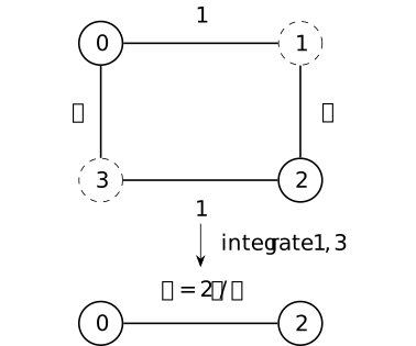
Solid circles are retained; dashed circles are integrated out. Orientations are suppressed because the quadratic energy is orientation independent. The bottom edge represents the induced coupling \(\beta \); its precision also has the diagonal term computed below.
The vectors \((1,1)^T/\sqrt 2\) and \((1,-1)^T/\sqrt 2\) diagonalize \(S\). Their eigenvalues are \[\begin {aligned} \sigma _+&=\alpha -\beta =\frac {s^2-(1+t)^2}{s}\\ &=\frac {a(a+2+2t)}{s},\\ \sigma _-&=\alpha +\beta =\frac {s^2-(1-t)^2}{s}\\ &=\frac {(a+2)(a+2t)}{s}. \end {aligned}\] Both are positive. The factorizations follow from \(s=1+t+a\); they also check positivity without appealing again to the general theorem. Put \[\mathcal D=a(a+2)(a+2t)(a+2+2t).\] Then \[\begin {aligned} \det C&=s^2,\qquad \det S=\mathcal D/s^2,\\ \det Q&=\det C\det S=\mathcal D,\\ c_C&=\frac {2\pi }{s},\qquad Z_S=\frac {2\pi s}{\sqrt {\mathcal D}},\\ Z_Q&=c_CZ_S=\frac {(2\pi )^2}{\sqrt {\mathcal D}}. \end {aligned}\] This reproduces the four-mode determinant and partition function. The effective action is \[\mathcal A_{\mathrm {eff}}(x)=\tfrac 12x^TSx+\log \frac {s}{2\pi }.\] Its constant records the integrated block.
A retained observable checks more than normalization. For \(F(x)=x_0x_2\), polynomial integrability and the marginal identity give \[\begin {aligned} \langle \phi _0\phi _2\rangle _Q &=\langle x_0x_2\rangle _S =(S^{-1})_{02}\\ &=\frac {\beta }{\alpha ^2-\beta ^2} =\frac {2ts}{\mathcal D}. \end {aligned}\] The indices \(0,2\) here name retained vertices. Inverting the displayed two-by-two matrix gives its off-diagonal entry \(\frac {\beta }{\det S}\), which proves the last equalities. Independently, the four-cycle spectral table gives \[\begin {aligned} 4\langle \phi _0\phi _2\rangle _Q &=\frac 1a-\frac 1{a+2}\\ &\quad -\frac 1{a+2t}+\frac 1{a+2+2t}\\ &=\frac {8ts}{\mathcal D}. \end {aligned}\] For the last equality, pair the first two terms and the last two: their difference has numerator \(2((a+2t)(a+2+2t)-a(a+2))=8ts\) over \(\mathcal D\). At \(t=m=1\), one obtains \[\begin {aligned} S&=\begin {pmatrix}7/3&-2/3\\-2/3&7/3\end {pmatrix},\\ S^{-1}&=\frac 1{15}\begin {pmatrix}7&2\\2&7\end {pmatrix},\\ \langle \phi _0\phi _2\rangle _Q&=\frac {2}{15},\\ c_C&=\frac {2\pi }{3},\quad Z_S=\frac {2\pi }{\sqrt 5},\quad Z_Q=\frac {4\pi ^2}{3\sqrt 5}. \end {aligned}\] Fixing the eliminated fields to zero instead gives precision \(A=3I_2\), covariance \(I_2/3\) and zero off-diagonal covariance. At \(t=2,m=1\), the same formulas give \[\begin {aligned} S&=\begin {pmatrix}11/4&-1\\-1&11/4\end {pmatrix},\\ \det S&=105/16,\\ S^{-1}&=\frac 1{105}\begin {pmatrix}44&16\\16&44\end {pmatrix}. \end {aligned}\] These are the parameters used in the symmetry comparison.
In the orthonormal sector coordinates \(x_\pm =(x_0\pm x_2)/\sqrt 2\) and \(y_\pm =(y_1\pm y_3)/\sqrt 2\), the couplings are \(-(1+t)\) and \(-(1-t)\). Their two eliminated pivots are both \(s\); each contributes \(\sqrt {2\pi/s}\), whose product is \(2\pi/s\). The factors \(1/\sqrt 2\) make these changes orthogonal, so there is no extra volume factor. The retained variance is \(\frac 12(\sigma _+^{-1}+\sigma _-^{-1})\), and the opposite covariance is \(\frac 12(\sigma _+^{-1}-\sigma _-^{-1})\). This agrees with the sector calculation.
There was no edge between vertices \(0\) and \(2\) in the supplied cycle. Elimination induces one in the effective quadratic form: \[S=\beta \begin {pmatrix}1&-1\\-1&1\end {pmatrix} +\sigma _+I_2.\] Thus \(\beta \) is an effective edge weight and \(\sigma _+\) an effective mass coefficient. This is a finite instance of fill-in: eliminating a single vertex joined to retained vertices with weights \(w_i\) and diagonal precision \(c>0\) subtracts \(ww^T/c\), creating off-diagonal entries \(-w_iw_j/c\) where no retained edge existed. The formula is the same Schur complement with \(H=-w\) and \(C=(c)\). Locality in the original graph need not survive elimination.
The half-turn preserves both sets \(R,U\) and swaps the two coordinates within each. For the swap matrix \(J\), the displayed \(S\) satisfies \(JSJ=S\); the induced two-site form retains this symmetry. The density and orthogonal-volume invariance then show that the retained law is invariant as well.
At \(m=0\), \(C=(1+t)I_2\) remains positive. Square completion and integration over the eliminated block still give \[S=\frac {2t}{1+t}\begin {pmatrix}1&-1\\-1&1\end {pmatrix}, \qquad c_C=\frac {2\pi }{1+t}.\] The retained constant mode has zero energy, so its full integral diverges by the kernel-box argument. The finite fiber factor cannot be divided by a finite retained partition function.
The global mean-zero law instead uses the space \(H=\{\phi :\sum _v\phi _v=0\}\) with its own induced volume. Its constraint \(x_0+x_2+y_1+y_3=0\) couples the two parts; \(H\) is neither their unrestricted product nor the product of their separate mean-zero lines. At \(t=1\), write a field in the three positive orthonormal modes as \(\phi =z_1u_1+z_2u_2+z_3u_3\). The coordinates are independent centered Gaussians of precisions \(2,2,4\). Put \[r=\frac {z_1+z_2}{\sqrt 2},\qquad v=\frac {z_1-z_2}{\sqrt 2}.\] This orthogonal change preserves \(z_1^2+z_2^2=r^2+v^2\) and two-dimensional volume. Thus \(r,v,z_3\) still have independent centered Gaussian laws of precisions \(2,2,4\). The retained unit coordinates satisfy \[\begin {aligned} x_-&=(\phi _0-\phi _2)/\sqrt 2=r,\\ x_+&=(\phi _0+\phi _2)/\sqrt 2=z_3/\sqrt 2. \end {aligned}\] Integrating the normalized \(v\) factor and changing variable \(z_3=\sqrt 2x_+\) give independent retained Gaussian densities of precisions \(2\) and \(8\). This density calculation identifies the law, not merely its covariance. Returning orthogonally to \((x_0,x_2)\) gives \[\begin {aligned} \operatorname {Cov}(x)&=\frac 1{16} \begin {pmatrix}5&-3\\-3&5\end {pmatrix},\\ Q_{H\to R}&=\begin {pmatrix}5&3\\3&5\end {pmatrix}. \end {aligned}\] These matrices multiply to the identity. The projected normalizer for this precision is \(\frac {2\pi }{\sqrt {16}}=\frac \pi 2\).
In contrast, directly setting \(m=0,t=1\) in the Schur formula gives the singular precision \(\begin {pmatrix}1&-1\\-1&1\end {pmatrix}\). Separately constraining that retained model to \(x_0+x_2=0\) leaves unit direction \((1,-1)/\sqrt 2\) with precision \(2\), normalizer \(\sqrt \pi \) and ambient covariance \(\frac 14\begin {pmatrix}1&-1\\-1&1\end {pmatrix}\). These are three distinct specified measures. The pinned affine law is another constraint with its own induced volume; fixing a vertex is not the marginal operation above.
The arithmetic pivot boundary is separate from the positive-real case. At \(m^2=1,t=-2\), \(s=t+2=0\), whereas \(\det Q=1\cdot 3\cdot (-3)\cdot (-1)=9\). Thus the full map can be invertible while this eliminated pivot is not. At \(t=-1\), the pivot exists but the later ratio denominator \(t+1\) vanishes. Neither value satisfies the positive-weight hypotheses used for the Gaussian laws here.