A supplied circle and a fixed Fourier mode [fdip-004G]
✍️sourceAGENTDRAFTED
- October 31, 2026
A supplied circle and a fixed Fourier mode [fdip-004G]
✍️sourceAGENTDRAFTED
- October 31, 2026
How does a finite operator approximate a differential operator when the circle and its length are already given? A periodic mesh, a normalized pairing and a positive mass give an explicit answer for each fixed Fourier mode. The same calculation controls one Gaussian second moment, using normalization and inverse-precision covariance. The spatial Dirac comparison provides related finite symbols; the scalar argument below does not require its Clifford module.
Definition 1. A circle mesh with normalized pairing [fdip-004H]AGENTDRAFTED
- October 31, 2026
Definition 1. A circle mesh with normalized pairing [fdip-004H]AGENTDRAFTED
- October 31, 2026
Supply the unit circle \(\mathbb R/\mathbb Z\), its coordinate \(x\) modulo one and length measure \(dx\). For an integer \(n\geq 3\), the circle mesh consists of the points \(j/n\), with \(j\in \mathbb Z/n\mathbb Z\), and spacing \(h_n=1/n\). Its real field space and reference pairing are \[E_n=\mathbb R^{\mathbb Z/n\mathbb Z},\qquad g_{0,n}(f,g)=\frac 1n\sum _{j=0}^{n-1}f_jg_j.\] On the complexification use \(\langle f,g\rangle _n=n^{-1}\sum _j\overline {f_j}g_j\); its restriction to real fields is \(g_{0,n}\).
Fix a mass squared \(\mu >0\), independent of \(n\). Define the cyclic shift, scaled nearest-neighbor Laplacian and precision by \[\begin {aligned} (T_nf)_j&=f_{j+1},\\ L_n&=n^2(2I-T_n-T_n^{-1}),\\ Q_n&=\mu I+L_n,\qquad q_n(f)=g_{0,n}(f,Q_nf). \end {aligned}\] Indices are taken modulo \(n\). These specialize the cyclic shift and difference energy, with the supplied scale \(n^2\). The scalar \(L_n\) is the nearest-neighbor operator compared with, and generally different from, the centered Dirac square in Proposition [fdip-000T].
Periodic reindexing gives \(T_n^*=T_n^{-1}\) in the normalized pairing. Consequently \[\langle f,L_nf\rangle _n =n\sum _{j=0}^{n-1}|f_{j+1}-f_j|^2\geq 0.\] Thus \(Q_n\geq \mu I\) and \(Q_n\) is invertible, including on constant fields. This is the positive precision convention with the declared \(g_{0,n}\), rather than a change of the action form.
The step-function interpolation \(I_n\) assigns to \(f\) the function with value \(f_j\) whenever \(j/n\leq x<(j+1)/n\), using the representative \(0\leq x<1\). It maps real or complex fields into \(L^2(\mathbb R/\mathbb Z,dx)\), the square-integrable functions modulo almost-everywhere equality. Each interval has length \(1/n\), so \[\|I_nf\|_{L^2}^2=\frac 1n\sum _j|f_j|^2=\|f\|_n^2.\] Thus the comparison preserves the specified norm.
Example 2. Fourier modes and their Gaussian moments on a circle mesh [fdip-004I]AGENTDRAFTED
- October 31, 2026
Example 2. Fourier modes and their Gaussian moments on a circle mesh [fdip-004I]AGENTDRAFTED
- October 31, 2026
For the circle mesh, let \(k\in \mathbb Z\) and set \[e_k(x)=e^{2\pi ikx},\qquad e_{n,k}(j)=e^{2\pi ikj/n}.\] Every entry has modulus one, hence \(\|e_{n,k}\|_n=1\). Applying the shift and its inverse directly gives \[\begin {aligned} T_ne_{n,k}&=e^{2\pi ik/n}e_{n,k},\\ L_ne_{n,k}&=\lambda _{n,k}e_{n,k},\\ \lambda _{n,k} &=n^2(2-e^{2\pi ik/n}-e^{-2\pi ik/n})\\ &=4n^2\sin ^2(\pi k/n). \end {aligned}\] This derives the scaled version of the nearest-neighbor symbol. Frequencies differing by \(n\) give the same samples. For fixed \(k\ne 0\), the condition \(n>2|k|\) separates \(k\) from \(-k\) modulo \(n\).
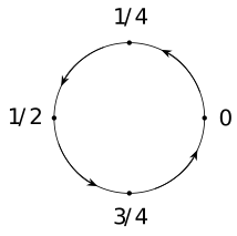
For \(k=0\), \(e_{n,0}=\mathbf 1\) and \(\lambda _{n,0}=0\). For \(k=1\), a four-point mesh has \(\lambda _{4,1}=32\); an eight-point mesh has \(\lambda _{8,1}=64(2-\sqrt 2)\). The picture shows the supplied unit circle sampled at 4 equally spaced points. Its arrows indicate increasing \(j\); they do not specify a dynamics.
Now use real fields and the Gaussian law \[d\nu _n(f)=Z_n^{-1}e^{-q_n(f)/2}\,d\operatorname {vol}_{g_{0,n}}(f).\] In raw coordinates the volume and normalization are \[\begin {aligned} d\operatorname {vol}_{g_{0,n}}&=n^{-n/2}\,df_0\cdots df_{n-1},\\ Z_n&=(2\pi )^{n/2}(\det Q_n)^{-1/2}. \end {aligned}\] The volume factor follows because \(f\mapsto f/\sqrt n\) is an orthonormal chart; the partition function is Theorem [fdip-002T]. The covariance operator relative to \(g_{0,n}\) is \(Q_n^{-1}\) by Theorem [fdip-000B]. Since the exponent is \(f^TQ_nf/(2n)\), the raw coordinate covariance matrix is \(nQ_n^{-1}\).
Define the complex Fourier observable \(a_{n,k}=n^{-1}\sum _j e^{-2\pi ikj/n}f_j\). It has zero mean. Writing \(v=e_{n,k}\) and \(v^*\) for its conjugate transpose, the coordinate covariance gives \[\begin {aligned} \mathbb E_{\nu _n}|a_{n,k}|^2 &=n^{-2}v^*(nQ_n^{-1})v\\ &=\frac 1{\mu +\lambda _{n,k}}, \end {aligned}\] because \(v^*v=n\). All real and imaginary parts and their products are integrable polynomials by Proposition [fdip-002W]. In particular the real mean \(a_{n,0}\) has variance \(1/\mu \). At \(k=1\), the four-point and eight-point second moments are respectively \((\mu +32)^{-1}\) and \((\mu +64(2-\sqrt 2))^{-1}\).
For \(k\ne 0\) and \(n>2|k|\), put \[\begin {aligned} c_{n,k}&=\operatorname {Re}a_{n,k} =\frac 1n\sum _j\cos (2\pi kj/n)f_j,\\ s_{n,k}&=-\operatorname {Im}a_{n,k} =\frac 1n\sum _j\sin (2\pi kj/n)f_j. \end {aligned}\] The geometric sum \(\sum _j e^{4\pi ikj/n}=0\): its ratio is not one, its \(n\)-th power is one, and multiplying the sum by one minus the ratio gives zero. Taking real and imaginary parts, and using the double-angle identities, gives normalized squared norms \(1/2\) for both the cosine and sine vectors and their orthogonality. Both vectors have precision eigenvalue \(\mu +\lambda _{n,k}\), so Theorem [fdip-000B] yields \[\operatorname {Var}(c_{n,k})=\operatorname {Var}(s_{n,k}) =\frac 1{2(\mu +\lambda _{n,k})}.\] The coefficients of the orthogonal projection \(A\cos (2\pi kj/n)+B\sin (2\pi kj/n)\) are \(A=2c_{n,k}\), \(B=2s_{n,k}\). Their variances are 4 times the displayed projection variances.
The character calculation and normalization above are direct
deductions from the cited finite operators and Gaussian results.
Mathlib's ZMod.dft uses the counting-measure forward sum;
\(a_{n,k}\) has the additional factor \(1/n\). This formal Fourier
transform is a supporting construction, not a formalization of the
mesh limit.
Proposition 3. A fixed Fourier mode and its massive inverse converge [fdip-004J]AGENTDRAFTED
- October 31, 2026
Proposition 3. A fixed Fourier mode and its massive inverse converge [fdip-004J]AGENTDRAFTED
- October 31, 2026
Use the circle meshes with fixed \(\mu >0\), and fix \(k\in \mathbb Z\) before letting \(n\to \infty \). For the Fourier modes and eigenvalues, \[\begin {aligned} \lambda _{n,k}&\longrightarrow 4\pi ^2k^2,\\ (\mu +\lambda _{n,k})^{-1} &\longrightarrow (\mu +4\pi ^2k^2)^{-1}. \end {aligned}\] Moreover, in \(L^2(\mathbb R/\mathbb Z,dx)\), \[I_nQ_n^{-1}e_{n,k} \longrightarrow (\mu +4\pi ^2k^2)^{-1}e_k.\] The vector on the right solves \(Au=e_k\) for \(A=-d^2/dx^2+\mu \) on smooth periodic functions. The selected Gaussian moment \(\mathbb E_{\nu _n}|a_{n,k}|^2\) converges to the same inverse eigenvalue.
Proof.
- October 31, 2026
Proof.
- October 31, 2026
For \(k=0\), the eigenvalue is identically zero and the sampled constant interpolates exactly to \(e_0=1\); all three assertions follow. For \(k\ne 0\), \[\lambda _{n,k} =4\pi ^2k^2\left (\frac {\sin (\pi k/n)}{\pi k/n}\right )^2.\] The sine quotient tends to one. Since \(\mu >0\), all denominators are at least \(\mu \), so continuity of inversion proves the scalar inverse limit.
For \(j/n\leq x<(j+1)/n\), the elementary inequality \(|e^{it}-e^{is}|\leq |t-s|\) gives \[|I_ne_{n,k}(x)-e_k(x)|\leq \frac {2\pi |k|}{n}.\] The inequality follows by integrating \(ie^{iu}\) between \(s\) and \(t\). The circle has measure one, hence the same bound holds for the \(L^2\) norm. Put \(b_n=(\mu +\lambda _{n,k})^{-1}\) and \(b=(\mu +4\pi ^2k^2)^{-1}\). Because \(|b_n|\leq 1/\mu \) and \(\|e_k\|_{L^2}=1\), \[\begin {aligned} \|b_nI_ne_{n,k}-be_k\|_{L^2} &\leq |b_n|\|I_ne_{n,k}-e_k\|_{L^2}+|b_n-b|\\ &\leq \frac {2\pi |k|}{\mu n}+|b_n-b|\longrightarrow 0. \end {aligned}\] The eigenvector equation identifies the left vector with \(I_nQ_n^{-1}e_{n,k}\). Differentiation gives \(Ae_k=(\mu +4\pi ^2k^2)e_k\). Finally the Gaussian second-moment formula in Example 2 is exactly \(b_n\).
This is an elementary limit deduction from the preceding finite
symbol, with an explicit interpolation map. Mathlib's
Real.tendsto_sin_div_nhdsNE_zero supplies the nonzero
sine-quotient limit used in the proof; the zero mode was handled
separately. The declaration does not supply the interpolation or
Gaussian comparison.
Remark 4. What the supplied-circle limit establishes [fdip-004K]AGENTDRAFTED
- October 31, 2026
Remark 4. What the supplied-circle limit establishes [fdip-004K]AGENTDRAFTED
- October 31, 2026
The fixed-mode limit compares finite operators and one Gaussian moment with a declared circle. Its length, measure, mesh spacing, factor \(n^2\) and positive mass are supplied. Without \(n^2\), each fixed-mode Laplacian eigenvalue tends to zero. This explains why a finite positive operator alone does not determine a continuum scale or geometry.
The quantifier on the frequency matters. For even \(n\) and \(k=n/2\), the discrete eigenvalue is \(4n^2\), whereas the continuum frequency has eigenvalue \(4\pi ^2k^2=\pi ^2n^2\). Their ratio stays \(4/\pi ^2\); the fixed-mode proof is therefore not a relative uniform estimate over all modes. It proves neither operator-norm resolvent convergence nor convergence of determinants or Gaussian measures. Removing the positive mass or adding interactions requires additional arguments.
For comparison, Weisz distinguishes the critical-point and phase-diagram control needed for low-energy lattice-QCD continuum limits from the renormalization questions for composite observables and high-energy scales [weisz2010renormalization, Section 1.1, printed p. 2]. The circle calculation is a much smaller prescribed approximation: it contains no interacting critical-point analysis. It establishes no emergent geometry, reflection positivity, Lorentzian reconstruction, Standard Model dynamics or gravitational dynamics. Those identifications remain among the open physical interfaces.