Gauge transfer operators at finite volume [fdip-007Y]
✍️sourceAGENTDRAFTED
- November 1, 2026
Gauge transfer operators at finite volume [fdip-007Y]
✍️sourceAGENTDRAFTED
- November 1, 2026
A positive character expansion turns a temporal plaquette weight into a positive operator on spatial link fields. Multiplication by half of the spatial weight on each side gives a transfer operator. Gauge averaging selects its physical states and retains the temporal links when the time direction closes into a circle.
The construction uses a finite spatial graph, normalized Haar measure and the positive kernel hypotheses. It proves finite periodic-time trace identities, a spectral Hamiltonian and link-reflected positivity for bounded spatial observables. The Gaussian transfer construction supplies the scalar comparison; reflection positivity by itself does not supply these operator and translation data.
Definition 1. Spatial link fields and their transfer kernel [fdip-007Z]AGENTDRAFTED
- November 1, 2026
Definition 1. Spatial link fields and their transfer kernel [fdip-007Z]AGENTDRAFTED
- November 1, 2026
Let \(G\) be a finite group, \(U(1)\) or \(SU(2)\), with normalized Haar measure. Fix a finite incidence presentation with vertex set \(V_s\), oriented edge set \(E_s\) and source and target maps \(s,t:E_s\to V_s\). The spatial configuration space and link Hilbert space are \[X=G^{E_s},\qquad \mathcal H_{\mathrm {link}}=L^2(X,dU;\mathbb C),\] where \(dU\) is product Haar probability measure. The gauge action of \(K=G^{V_s}\) is \[(h\cdot U)_e=h_{t(e)}U_eh_{s(e)}^{-1},\qquad (R_hf)(U)=f(h^{-1}\cdot U).\] Haar invariance makes every \(R_h\) unitary.
Choose a real continuous central kernel \(k\) satisfying the positive coefficient conditions: \[\begin {gathered} k(g)>0,\qquad k(g^{-1})=k(g),\\ k(g)=\sum _{\rho \in \widehat G}d_\rho a_\rho \chi _\rho (g), \qquad a_\rho >0,\qquad \sum _{\rho \in \widehat G}d_\rho ^2a_\rho <\infty . \end {gathered}\] All irreducible representations here are complex and unitary. The expansion is uniformly absolutely convergent. Pointwise positivity and coefficient positivity are separate hypotheses.
Let \(V:X\to \mathbb R\) be continuous and gauge invariant, and set \(b(U)=e^{-V(U)/2}\). Compactness makes \(b\) and \(b^{-1}\) bounded. If \(M_b\) denotes multiplication by \(b\), define \[\begin {aligned} c(U,U')&=\prod _{e\in E_s}k(U_eU_e'^{-1}),\\ (C_kf)(U)&=\int _Xc(U,U')f(U')\,dU',\\ T&=M_bC_kM_b. \end {aligned}\] This is the pure-gauge transfer operator for the specified data. Its integral kernel is \(b(U)c(U,U')b(U')\). The spatial potential may be a sum of Wilson plaquette terms, but the definition only needs its stated invariance and continuity.
The factorization separates the two spatial half-weights from the temporal convolution. It parallels the gauge factors in [luscher1977transfer, Eqs. (17), (20)–(21), p. 287]; the source comparison distinguishes this pure-gauge model from that paper's gauge and fermion construction.
Example 2. Positive temporal weights for signs and phases [fdip-0081]AGENTDRAFTED
- November 1, 2026
Example 2. Positive temporal weights for signs and phases [fdip-0081]AGENTDRAFTED
- November 1, 2026
The transfer kernel conditions have elementary examples. For \(G=\mathbb Z_2=\{1,-1\}\) and \(\beta >0\), take \(k(u)=e^{\beta u}\). The two characters are \(1\) and \(u\), and \[k(u)=\cosh \beta +u\sinh \beta .\] Thus \(a_{\mathrm {triv}}=\cosh \beta >0\) and \(a_{\mathrm {sgn}}=\sinh \beta >0\). Both dimensions are one, so the coefficient sum is \(e^\beta \). The function is real, strictly positive and invariant under inversion.
For \(G=U(1)\), the Wilson and Villain weights give two choices: \[\begin {aligned} k_W(e^{i\theta })&=e^{\beta \cos \theta }, &a_n^W&=I_n(\beta ),\\ k_V(e^{i\theta })&=\sum _{\ell \in \mathbb Z} e^{-\beta _V(\theta -2\pi \ell )^2/2}, &a_n^V&=\frac {e^{-n^2/(2\beta _V)}}{\sqrt {2\pi \beta _V}}. \end {aligned}\] Here \(\beta ,\beta _V>0\) and \(n\in \mathbb Z\). All coefficients are positive and summable; all characters have dimension one. The cited calculation proves the series, continuity and inversion symmetry. Each function is strictly positive from its definition, so every hypothesis is met. These are unnormalized weights; no zeroth coefficient has been divided out.
At \(\beta =0\), the sign or Wilson weight is constant and its nontrivial Fourier coefficients vanish. The resulting convolution kills nonconstant modes, so strict coefficient positivity cannot be removed from the injectivity assertion in Theorem 4.
Proposition 3. A positive coefficient expansion on SU(2) [fdip-0082]AGENTDRAFTED
- November 1, 2026
Proposition 3. A positive coefficient expansion on SU(2) [fdip-0082]AGENTDRAFTED
- November 1, 2026
Let \(f\) be the defining two-dimensional representation of \(SU(2)\) and \(\beta >0\). Then \[k(g)=e^{\beta \chi _f(g)}\] satisfies the transfer kernel conditions. More precisely, if \(m_\rho (n)\) is the multiplicity of \(\rho \) in \(f^{\otimes n}\), then \[\begin {aligned} c_\rho &=\sum _{n=0}^\infty \frac {\beta ^n}{n!}m_\rho (n)>0,\\ a_\rho &=\frac {c_\rho }{d_\rho },\qquad \sum _\rho d_\rho ^2a_\rho =e^{2\beta }. \end {aligned}\] This is the tensor-power argument used in [luscher1977transfer, Proposition 1, p. 288], with strict occurrence and absolute convergence justified below.
Proof.
- November 1, 2026
Proof.
- November 1, 2026
The matrix description of SU(2) writes its elements as \[g=\begin {pmatrix}z&w\\-\overline w&\overline z\end {pmatrix}, \qquad |z|^2+|w|^2=1.\] Hence \(\chi _f(g)=2\operatorname {Re}z\) is real, \(\chi _f(g^{-1})=\chi _f(g)\), and \(k\) is continuous, central and strictly positive. Every tensor power is unitary; invariant orthogonal complements decompose it into irreducibles. Therefore \[\chi _f(g)^n=\sum _\rho m_\rho (n)\chi _\rho (g), \qquad \sum _\rho m_\rho (n)d_\rho =2^n.\] Expanding the exponential and using nonnegative multiplicities gives \[\sum _\rho d_\rho c_\rho =\sum _{n=0}^\infty \frac {\beta ^n2^n}{n!}=e^{2\beta }.\] Since \(|\chi _\rho (g)|\le d_\rho \), this also justifies rearranging the series uniformly and proves the claimed expansion. It remains to show that no \(c_\rho \) is zero.
Consider the algebra of finite linear combinations of matrix
coefficients of the powers \(f^{\otimes n}\), including \(n=0\).
Products are coefficients of tensor products, so this is a unital
algebra of continuous functions. The entries of \(g\) distinguish
its points. Their complex conjugates are again entries up to a
sign, by the displayed matrix form, so the algebra is closed under
complex conjugation. The complex Stone–Weierstrass theorem makes
it uniformly dense in \(C(SU(2),\mathbb C)\). Here that analytic
theorem is used as a cited statement: a conjugation-closed unital
subalgebra of continuous complex functions on a compact space is
dense if it separates points. Its exact formal statement is
ContinuousMap.starSubalgebra_topologicalClosure_eq_top_of_separatesPoints.
The reference supplies this density theorem, not the representation
argument that follows.
If an irreducible \(\rho \) occurred in no tensor power, Schur orthogonality from the Peter–Weyl theorem would make all its matrix coefficients orthogonal to this algebra. Choose a nonzero such coefficient \(u\). Uniform density gives algebra functions converging uniformly, hence in normalized Haar \(L^2\), to \(u\). Orthogonality would then give \(\|u\|_2^2=0\), a contradiction. Thus \(m_\rho (n)>0\) for some \(n\), and \(\beta >0\) makes \(c_\rho >0\). Dividing by \(d_\rho \) proves all remaining coefficient assertions.
Theorem 4. Positivity and trace class of the gauge transfer operator [fdip-0080]AGENTDRAFTED
- November 1, 2026
Theorem 4. Positivity and trace class of the gauge transfer operator [fdip-0080]AGENTDRAFTED
- November 1, 2026
For the spatial transfer data, \(C_k\) and \(T=M_bC_kM_b\) are bounded, self-adjoint, positive, injective and trace class. Both commute with every gauge operator \(R_h\). If \[\kappa =\sum _\rho d_\rho ^2a_\rho =k(1),\] then \[\operatorname {Tr}C_k=\kappa ^{|E_s|},\qquad \operatorname {Tr}T\le \|b\|_\infty ^2\kappa ^{|E_s|}.\] Positive means \(\langle f,Tf\rangle \ge 0\); in fact this pairing is strictly positive for every nonzero \(f\). It does not assert a uniform positive lower bound on the spectrum.
Proof.
- November 1, 2026
Proof.
- November 1, 2026
For one edge, use the normalized matrix-entry basis \(\phi _{\rho ij}(U)=\sqrt {d_\rho }\rho (U)_{ij}\) of the Peter–Weyl theorem. Unitarity gives \[k(UU'^{-1})=\sum _{\rho ,i,j} a_\rho \phi _{\rho ij}(U)\overline {\phi _{\rho ij}(U')}.\] Indeed, the matrix-entry sum is \(d_\rho \operatorname {Tr}(\rho (U)\rho (U')^*)\). Schur orthogonality therefore makes convolution act by \(a_\rho \) on this block. The tensor products of these bases over the finitely many edges give an orthonormal basis \((\phi _I)\) of \(\mathcal H_{\mathrm {link}}\), with eigenvalues \[\alpha _I=\prod _{e\in E_s}a_{\rho _e}>0,\qquad \sum _I\alpha _I=\kappa ^{|E_s|}<\infty .\] The operator assertions about \(C_k\), including injectivity and its trace, follow directly from this complete diagonalization. Here trace class for a positive compact operator has the meaning used in the Gaussian spectrum: its eigenvalues are summable.
For clarity, write the rank-one operator \(|v\rangle \langle v|\) as \(f\mapsto v\langle v,f\rangle \), with the inner product linear in its second variable. Then \[T=\sum _I\alpha _I |b\phi _I\rangle \langle b\phi _I|.\] The trace norm is \(\|A\|_1=\operatorname {Tr}((A^*A)^{1/2})\); for a positive operator it equals its trace. Trace class means this norm is finite. Each summand is positive and its trace norm is \(\alpha _I\|b\phi _I\|_2^2\). Their sum is at most \(\|b\|_\infty ^2\sum _I\alpha _I\), so the series converges in trace norm and proves positivity, self-adjointness, compactness and the trace bound. For \(f\ne 0\), bounded invertibility of \(M_b\) gives \(bf\ne 0\); hence \[\langle f,Tf\rangle =\langle bf,C_kbf\rangle >0.\] This proves injectivity as well.
Under a simultaneous gauge change of \(U,U'\), \[(h\cdot U)_e(h\cdot U')_e^{-1} =h_{t(e)}(U_eU_e'^{-1})h_{t(e)}^{-1}.\] Centrality of \(k\) and invariance of product Haar measure show \(C_kR_h=R_hC_k\). Gauge invariance of \(b\) gives the same commutation for \(M_b\) and \(T\).
The coefficient calculation is a direct application of
Peter–Weyl orthogonality. TauCeti's
TauCeti.peterWeylBlockAveraging_eq_starProjection
identifies character averaging with the corresponding orthogonal
block projection. Its kernel is \(d_\rho \overline {\chi _\rho }\)
and its matrix-coefficient convention is the conjugated one
explained in Theorem [fdip-007C]. Reindexing by dual representations
aligns the conventions; reality and inversion symmetry give
\(a_{\overline \rho }=a_\rho \). This correspondence concerns the
block projection, while the positive weighted sum and spatial
multipliers are proved above.
The factorization proof follows the idea of [luscher1977transfer, Proposition 1, p. 288], under the explicit pure-gauge hypotheses of Definition 1.
Theorem 5. Gauge projection and periodic-time traces [fdip-0083]AGENTDRAFTED
- November 1, 2026
Theorem 5. Gauge projection and periodic-time traces [fdip-0083]AGENTDRAFTED
- November 1, 2026
For the spatial transfer data, normalized gauge averaging is the orthogonal projection \[\begin {aligned} (Pf)(U)&=\int _K f(h^{-1}\cdot U)\,dh,\\ \mathcal H_{\mathrm {phys}} &=\{f:R_hf=f\text { for every }h\in K\}=P\mathcal H_{\mathrm {link}}. \end {aligned}\] This defines the physical Hilbert space of neutral states. The restriction \(T_{\mathrm {phys}}=T|_{\mathcal H_{\mathrm {phys}}}\) is positive, injective and trace class. It is nonzero since constants belong to \(\mathcal H_{\mathrm {phys}}\). For every integer \(N\ge 1\), \[Z_N=\operatorname {Tr}_{\mathrm {phys}}T_{\mathrm {phys}}^N =\operatorname {Tr}_{\mathrm {link}}(PT^N)>0.\] The gauge projector is part of the periodic trace.
There is an explicit lattice integral for \(Z_N\). Put \(U_N=U_0\), take independent variables \(U_j\in X\) and \(h_j\in K\) for \(0\le j<N\), and define \[\begin {aligned} B_{j,e}&=U_{j,e}h_{j,s(e)}U_{j+1,e}^{-1}h_{j,t(e)}^{-1},\\ \mathcal W_N(U,h)&= \prod _{j=0}^{N-1}e^{-V(U_j)} \prod _{j=0}^{N-1}\prod _{e\in E_s}k(B_{j,e}). \end {aligned}\] Then, with normalized product Haar measures, \[Z_N=\int _{X^N\times K^N}\mathcal W_N(U,h)\,dU\,dh.\] Thus \(Z_N^{-1}\mathcal W_N\,dU\,dh\) is a probability law. The temporal link \(h_{j,v}\) transports from time \(j+1\) back to time \(j\). For \(N=1,2\), the formula retains the indexed temporal steps; it does not identify them with edges of an ordinary simple cycle.
For independent gauge changes \(g_j\in K\), with \(g_N=g_0\), the transformations are \[\begin {aligned} U_j&\longmapsto g_j\cdot U_j,\\ h_{j,v}&\longmapsto g_{j,v}h_{j,v}g_{j+1,v}^{-1}. \end {aligned}\] Each \(B_{j,e}\) is conjugated by \(g_{j,t(e)}\). Therefore the weight and measure are invariant. If \(f_j:X\to \mathbb C\) are bounded measurable gauge-invariant functions, multiplication by \(f_j\) preserves \(\mathcal H_{\mathrm {phys}}\), and \[\mathbb E_N\prod _{j=0}^{N-1}f_j(U_j) =\frac {\operatorname {Tr}_{\mathrm {phys}} (M_{f_0}T_{\mathrm {phys}}\cdots M_{f_{N-1}}T_{\mathrm {phys}})}{Z_N}.\] This is a finite periodic-time identity for the specified spatial observables, with the temporal links integrated as above.
Proof.
- November 1, 2026
Proof.
- November 1, 2026
Fubini and Jensen define \(P\) on \(L^2\) and give \(\|P\|\le 1\). Haar invariance gives \(P^2=P\); inversion of \(h\) gives \(P^*=P\). Translating the averaging variable shows that its image is fixed by each \(R_h\), while averaging a fixed vector leaves it unchanged. These are Hilbert-space equalities; no common pointwise representative for all group elements is required. By Theorem 4, \(T\) commutes with \(P\). Its restriction is therefore positive and trace class, and \(\langle f,Tf\rangle >0\) for nonzero physical \(f\) proves injectivity there. Set \(S=PT=PTP\) on the full link space. It acts as \(T_{\mathrm {phys}}\) on the physical space and as zero on its orthogonal complement, so \(S^N=PT^N\) has the asserted physical trace.
Averaging the first variable of the kernel of \(T\) gives the continuous kernel of \(S\): \[L(U,U')=b(U)b(U')\int _K \prod _e k(U_eh_{s(e)}U_e'^{-1}h_{t(e)}^{-1})\,dh.\] To obtain this expression, use invariance of \(b\) and move \(h_{t(e)}^{-1}\) from the front of the kernel argument to its end by centrality. Every factor is strictly positive.
The diagonal trace formula, including the case \(N=1\), can be justified directly. The rank-one expansion in Theorem 4 gives \[S=\sum _I\alpha _I |P(b\phi _I)\rangle \langle P(b\phi _I)|\] in trace norm. Its kernel expansion converges uniformly when summed over finite sets of representation blocks. For one edge, unitarity gives \[\sum _{i,j}|\phi _{\rho ij}(U)|^2=d_\rho ^2.\] For the finite edge product, the diagonal sum over a tail of blocks is therefore the corresponding tail of \(\sum _I\alpha _I=\kappa ^{|E_s|}\), uniformly in \(U\). Cauchy–Schwarz gives the same bound off the diagonal. Multiplying by \(b\) and averaging in both variables preserve uniform convergence. Integrating the diagonal term by term consequently gives \[\int _XL(U,U)\,dU =\sum _I\alpha _I\|P(b\phi _I)\|_2^2 =\operatorname {Tr}S.\] Multiplication by a bounded function permits the same argument for \(\operatorname {Tr}(M_fS)\).
For \(N\ge 2\), the Hilbert–Schmidt kernel trace identity of Theorem [fdip-007V] gives \[\operatorname {Tr}(M_{f_0}S\cdots M_{f_{N-1}}S) =\int _{X^N}\prod _j f_j(U_j)L(U_j,U_{j+1})\,dU.\] All kernels are bounded on compact spaces, so repeated integrals are absolutely convergent. The same formula for \(N=1\) was proved by the diagonal expansion. Gauge-invariant multiplication commutes with \(P\); hence this full-space trace equals the physical-space trace in the statement. Expanding each \(L\) with an independent \(h_j\) gives \(\mathcal W_N\), because the two adjacent factors \(b(U_j)\) combine to \(e^{-V(U_j)}\). Taking every \(f_j=1\) proves the partition function; general \(f_j\) prove the expectation identity. Strict positivity and compactness of the weight give \(0<Z_N<\infty \). The displayed gauge transformation conjugates \(B_{j,e}\) by direct cancellation, which proves the final invariance assertion.
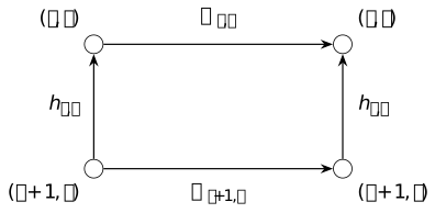
The temporal plaquette based at \((j,t)\) is traversed down the right edge, backwards along the bottom, up the left edge and then along the top. With the transport order, the first transport acts on the right and the product is exactly \(B_{j,e}\). Temporal averaging is retained at every step, so no periodic gauge-fixing assumption removes \(P\).
Example 6. Why the periodic trace needs gauge projection [fdip-0084]AGENTDRAFTED
- November 1, 2026
Example 6. Why the periodic trace needs gauge projection [fdip-0084]AGENTDRAFTED
- November 1, 2026
Take a graph with one edge and two distinct vertices, with \(G=\mathbb Z_2\), \(V=0\) and the sign kernel \(k(u)=e^{\beta u}\), \(\beta >0\). The link space has orthonormal basis \(1,u\), with \[T1=(\cosh \beta )1,\qquad Tu=(\sinh \beta )u.\] The two endpoint gauge transformations act by \(u\mapsto h_tuh_s\). Their action is transitive on the two link configurations. Thus the gauge projector satisfies \(P1=1\) and \(Pu=0\), and the physical space consists exactly of constants.
For every \(N\ge 1\), the projected and unprojected traces are \[\begin {aligned} \operatorname {Tr}(PT^N)&=(\cosh \beta )^N,\\ \operatorname {Tr}(T^N)&=(\cosh \beta )^N+(\sinh \beta )^N. \end {aligned}\] They are different because \(\beta >0\). In the temporal-link integral, each independent endpoint average gives \[\frac 14\sum _{h_s,h_t=\pm 1} e^{\beta U h_sU'h_t}=\cosh \beta .\] The remaining normalized link integrals contribute one, reproducing the projected answer. Dropping \(P\) would retain the nonphysical sign mode and change this finite periodic law.
Corollary 7. The physical spectral Hamiltonian [fdip-0085]AGENTDRAFTED
- November 1, 2026
Corollary 7. The physical spectral Hamiltonian [fdip-0085]AGENTDRAFTED
- November 1, 2026
For the physical transfer operator, let \(\lambda _0=\|T_{\mathrm {phys}}\|>0\) and fix a time step \(a_t>0\). There is an orthonormal eigenbasis \((\psi _j)\) with \(0<\lambda _j\le \lambda _0\), including an eigenvector at \(\lambda _0\). Define \[\widehat T=\frac {T_{\mathrm {phys}}}{\lambda _0},\qquad E_j=\frac 1{a_t}\log \frac {\lambda _0}{\lambda _j}.\] The transfer Hamiltonian is \(H=-a_t^{-1}\log \widehat T\), with the explicit domain and action \[\begin {aligned} D(H)&=\left \{f=\sum _jc_j\psi _j: \sum _jE_j^2|c_j|^2<\infty \right \},\\ Hf&=\sum _jE_jc_j\psi _j. \end {aligned}\] It is nonnegative and self-adjoint, and \(e^{-a_tH}=\widehat T\). If the physical Hilbert space is infinite dimensional, \(H\) is unbounded. This assertion does not specify the multiplicity of its zero eigenspace.
Proof.
- November 1, 2026
Proof.
- November 1, 2026
The spectral theorem for compact self-adjoint operators applies to the positive trace-class operator of Theorem 5. Injectivity removes its zero eigenspace, so the positive eigenvectors form a complete orthonormal basis. Its nonzero norm is an eigenvalue. In the finite-dimensional case the list is finite; otherwise its eigenvalues tend to zero.
The eigenspace-density assertion is formalized by
ContinuousLinearMap.orthogonalComplement_iSup_eigenspaces_eq_bot:
for a compact symmetric operator on a complete real or complex
inner-product space, the span of all eigenspaces has zero orthogonal
complement. This reference supplies that spectral premise; the
logarithm, its domain and its core are addressed below.
Under the unitary coefficient map \(f\mapsto (c_j)\), the normalized transfer is multiplication by \(\lambda _j/\lambda _0\). Its spectral logarithm is therefore multiplication by the real nonnegative sequence \(E_j\) on the stated maximal domain. This diagonal operator is self-adjoint; finite coefficient truncations form a core. Exponentiating on the basis proves the transfer identity. If the list is infinite, \(\lambda _j\to 0\) implies \(E_j\to \infty \), proving unboundedness.
This is the same normalization and domain construction as the Gaussian oscillator, without its explicit eigenvalues. It supplies a Hamiltonian at finite spatial volume. A unique vacuum, limits in time or volume, and a continuum field theory are separate questions, not conclusions of this spectral construction.
Theorem 8. Link reflection as a trace square [fdip-0086]AGENTDRAFTED
- November 1, 2026
Theorem 8. Link reflection as a trace square [fdip-0086]AGENTDRAFTED
- November 1, 2026
Use the periodic gauge law with \(N=2m\), \(m\ge 1\). Reflect time by \(\theta (j)=1-j\) modulo \(2m\); the positive half is \(\{1,\ldots ,m\}\). As in the scalar definition, this is a link reflection: its cuts lie between times \(0,1\) and \(m,m+1\).
Let \(\mathcal A_+\) consist of finite linear combinations of functions \[F(U)=\prod _{j=1}^m f_j(U_j),\] where each \(f_j:X\to \mathbb C\) is bounded, measurable and gauge invariant. These form an algebra of spatial observables. For such a product, on \(\mathcal H_{\mathrm {phys}}\) define \[A_F=T_{\mathrm {phys}}^{1/2}M_{f_1}T_{\mathrm {phys}} M_{f_2}\cdots T_{\mathrm {phys}}M_{f_m} T_{\mathrm {phys}}^{1/2},\] where for \(m=1\) this means \(T_{\mathrm {phys}}^{1/2}M_{f_1}T_{\mathrm {phys}}^{1/2}\). Extend this assignment linearly to finite sums. Then \(A_F\) is Hilbert–Schmidt and \[\mathbb E_{2m}\left [\overline {F(\theta U)}F(U)\right ] =\frac {\operatorname {Tr}(A_F^*A_F)}{Z_{2m}}\ge 0, \qquad (\theta U)_j=U_{1-j}.\] The temporal links have already been integrated in the periodic trace identity. No assertion about arbitrary observables involving individual temporal links is included.
Proof.
- November 1, 2026
Proof.
- November 1, 2026
The positive trace-class operator \(T_{\mathrm {phys}}\) has a Hilbert–Schmidt square root. Every multiplication operator here is bounded, as are all intervening transfer factors, so \(A_F\) is Hilbert–Schmidt; the same holds for a finite sum.
For products \(F=\prod _j f_j(U_j)\) and \(G=\prod _j g_j(U_j)\), the adjoint reverses the order and conjugates each multiplier. The bounded trace formula and cyclicity of a trace-class product give \[\operatorname {Tr}(A_F^*A_G) =Z_{2m}\,\mathbb E_{2m} \left [\overline {F(\theta U)}G(U)\right ].\] The cyclic order of the multipliers is \[\overline f_m,\ldots ,\overline f_1,g_1,\ldots ,g_m,\] with one full transfer between adjacent entries. They occur at times \(m+1,\ldots ,2m,1,\ldots ,m\), where \(2m=0\); hence \(f_j\) is conjugated at time \(1-j\). There are exactly \(2m\) transfer factors after the adjacent half-powers combine.
Expanding finite sums proves the same sesquilinear identity for all \(F,G\in \mathcal A_+\). If two product-sum presentations define the same function, their difference has zero expectation against its reflected conjugate, and the identity makes the corresponding difference of operators have Hilbert–Schmidt norm zero. Thus \(A_F\) is independent of that presentation. Taking \(G=F\) proves the trace-square identity and positivity.
This proof uses the explicitly positive operator of Theorem 4 and the exact finite-time law of Theorem 5. It does not reverse the argument to reconstruct a transfer operator from an arbitrary reflection-positive law; the scalar quotient obstruction shows why that distinction matters.
Remark 9. The scope of the finite gauge construction [fdip-0087]AGENTDRAFTED
- November 1, 2026
Remark 9. The scope of the finite gauge construction [fdip-0087]AGENTDRAFTED
- November 1, 2026
The positive convolution theorem and projected finite-time trace law concern a specified pure-gauge model on a finite spatial graph. Their assumptions are the strictly positive, summable character coefficients of Definition 1, not reflection positivity alone. The trace-square theorem applies to the stated algebra of bounded gauge-invariant spatial observables.
Lüscher's construction includes \(SU(N)\) gauge fields and Wilson fermions. Proposition 1 proves self-adjointness, boundedness, gauge invariance and strict positivity of its transfer operator. Its factorization and argument using tensor characters motivate the pure-gauge proof here. The fermion factors require the stated hopping assumptions, including \(0<K_{\mathrm {hop}}<1/6\); \(K_{\mathrm {hop}}\) is that paper's hopping parameter, not the spatial gauge group \(K\) used here. See [luscher1977transfer, pp. 286–288, Proposition 1].
Proposition 2 in [luscher1977transfer, p. 289] identifies time-ordered expectations under its specified gauge fixing and boundary conditions: periodic gauge fields and anticyclic fermions in time. The qualification on periodic temporal gauge appears in footnote 3 on p. 285. The direct projected integral of Theorem 5 retains temporal averaging, rather than using that gauge-fixing identification as a finite-periodic premise.
The spectral Hamiltonian has its stated maximal domain; boundedness of the transfer operator does not make its logarithm bounded. No unique-vacuum or continuum reconstruction claim is required. In particular, the joint Gaussian matter law and lattice fermion operators need their own transfer and positivity hypotheses.