Let \(\mathcal C_{\rm act}\) be an active-context space, \(\mathcal Z_{\rm man}\) an explicitly managed computation-state space, and \(\mathcal H_{\rm pers}\) a persistent harness-state space. A four-layer harness state is

The coordinates are, respectively, the executable model artifact, the token-visible context, explicitly managed values or sessions, and state that can survive the present invocation. A transition may change any declared subset of these coordinates. A fixed-weight harness transition holds \(M\) fixed while changing one or more of \(c,z,h\).

Prime Agent Section 2.2 names model weights, active context, explicitly managed computation, and retained state as levels L0--L3, and describes the operations that move information between them [karten2026prime, Section 2.2]. The formulation in Definition 1.1.1 preserves that operational separation without treating the labels as an ordering of intelligence or capability.

Two runs with identical weights and different persistent state can induce different policies. That observation does not say that either run acquired a new circuit in the fixed artifact, and it does not compare their independently evaluated utility.

Let \(\mathcal I_{\rm har}\) be a content-identifier space. A versioned harness configuration is a finite record \(\kappa ^{\rm har}\in \mathcal I_{\rm har}\) that resolves the active-context assembly rule, managed-computation interface, tool permissions, session and message semantics, compaction policy, persistent-state schema, refinement policy, recovery rule, and implementation versions.

Together with a state \(\Xi \), the record resolves a non-anticipating harness policy. Changing one field produces a different declared intervention even when the executable model artifact is unchanged. The record does not include an evaluation binding; that is a separate record coordinate.

Fix a finite event alphabet \(\mathcal E_{\rm har}\). A persistent event stream of length \(n\) is

The append operation is \(L_{n+1}=\operatorname {append}(L_n,e_n)\). Write \(L_i\preceq _{\rm pref}L_j\) when \(L_i\) is a prefix of \(L_j\). An append-only stream satisfies \(L_i\preceq _{\rm pref}L_j\) for every \(i\leq j\); branching creates distinct continuations with a common prefix rather than rewriting that prefix.

Events may record model or tool calls, messages, interventions, retries, verifier outcomes, harness edits, and resource use. The event schema and its exact version belong to the configuration of Definition 1.1.3.

Let \(\mathcal V_{\rm fold}\) be a space of fold versions. For each \(v\in \mathcal V_{\rm fold}\), fix a deterministic map

Given an initial persistent state \(h_0\), event stream \(L_n=(e_0,\ldots ,e_{n-1})\), and version sequence \(\boldsymbol v=(v_0,\ldots ,v_{n-1})\), its materialized harness state is obtained recursively by

The materialization record is the tuple \((h_0,L_n,\boldsymbol v,(F_v)_v)\). Omitting a version or the initial state defines a family of possible materializations, not one replayable state.

For a materialization record in Definition 1.1.5, replaying the same initial state, event sequence, version sequence, and fold maps produces the same state \(h_n\).

This finite result follows from the displayed hypotheses. It assumes exact equality of all recorded inputs and deterministic fold maps.

The result in Theorem 1.1.6 is an identity about a declared transition system. It does not show that the event stream is complete, that an external process can be reconstructed, that the fold is faithful to the environment, or that the resulting state is useful or safe.

Prime Agent reports append-only events, versioned state, recovery, and rollback in Sections 2.2 and 2.5 [karten2026prime, Sections 2.2 and 2.5]. Those implementation claims motivate the event record; Theorem 1.1.6 proves the finite replay identity directly from the declared transition rule.

The same executable artifact can be paired with two persistent states and therefore two resolved harness policies. The harness state changes while the executable model remains fixed.

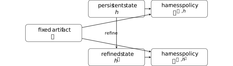
Different policies here establish only that harness state is an intervention coordinate. An independent evaluation is still required to compare their outcomes.

Prime Agent Section 2.5 uses the phrase ``self-improvement'' for execution evidence converted into persistent prompts, memories, skills, or subagent specifications while model weights remain fixed [karten2026prime, Section 2.5]. In the notation of Definition 1.1.1, this is a change to \(h\) with \(M\) held fixed.

The term therefore does not establish a change to the model artifact, a new learned circuit, or capability acquisition in the sense of Definition [ftip-0007]. It describes persistent harness adaptation.

An evaluation configuration record is a finite record \(\mathfrak e\) that resolves the task and instance law, environment and tool interfaces, executable model artifact, serializer and inference policy, harness configuration, compaction and refinement policies, retry rule, completion gate, evaluator, seed law, and componentwise resource limits.

Together with the independent evaluation interface of Convention [ftip-005D], the record determines the law of a stopped evaluation run and its realized cost vector. A reported score is the pair consisting of the statistic and the exact record \(\mathfrak e\); a scalar without its record is an under-specified family of measurements.

Section 2.6 of [karten2026prime] binds task and tool interfaces to model settings. Its evaluation configuration also records compaction, refinement, retry, completion, and resource policies. The record in Definition 1.2.1 is a proposed representation of those configuration choices.

To attribute a score difference to a harness coordinate, the comparison must hold the other coordinates fixed or model their changes explicitly. Two scores under different records \(\mathfrak e\) and \(\mathfrak e'\) can still be descriptively useful, but their difference does not isolate a causal harness effect.

A session lineage tree is a finite rooted directed tree \(\mathcal T=(V,E,r)\) whose edges point from a parent session to a directly spawned descendant. Each node \(v\in V\) carries an immutable session identifier, its resolved harness and inference stamps, a local event stream, and a local realized cost \(c_v\in \mathbb R_+^m\).

For a node \(v\), let \(\mathcal T_v\) be the induced subtree containing \(v\) and all its descendants. Distinct children of one node have disjoint node sets. Messages between branches are events in their local streams and do not merge their identities or costs.

For a session lineage tree Definition 1.2.3, its descendant-complete cost is the componentwise sum

The local cost \(c_v\) contains only work assigned to node \(v\); a model or tool call is charged to exactly one node. The vector retains its declared units and embeds into the lifecycle account of Definition [ftip-005H]. A scalar price can be applied only after the vector is formed.

Let the root \(r\) of a finite lineage tree have children \(v_1,\ldots ,v_k\). Then

This finite accounting identity follows from assigning each local cost to exactly one node.

Fix a componentwise hard budget \(b\in \mathbb R_+^m\). After accumulated cost \(a\preceq b\), a proposed continuation has a declared worst-case cost bound \(\bar c\in \mathbb R_+^m\). It is budget-admissible when

If admitted, the continuation must either stop within a realized cost \(c\preceq \bar c\) or report a contract violation. Rejected proposals may have a separately accounted proposal cost, which must already be included in \(a\) before the admission test.

Consider a finite sequence of continuations. Start from \(a_0\preceq b\). At step \(i\), admit only if \(a_i+\bar c_i\preceq b\), and require the realized cost to satisfy \(c_i\preceq \bar c_i\). With \(a_{i+1}=a_i+c_i\), every accumulated cost satisfies \(a_i\preceq b\).

This finite result is a contract theorem, not a prediction that a real executor respects its declared bound.

Use two cost coordinates, such as output tokens and tool calls. The root delegates to two children, and one child delegates once more.

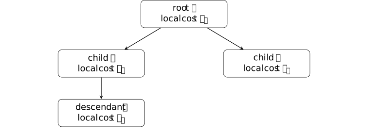
The cost of a child subtree is its local cost plus the costs of all descendants. Therefore

Charging only the root hides descendant work; charging a descendant again as a separate parent-local cost double counts it.

Prime Agent Section 3.1 places native-harness runs beside externally reported ARC-AGI-3 results and explicitly says the external points situate the curves rather than isolate a causal harness effect [karten2026prime, Section 3.1]. That is an empirical comparison under multiple evaluation records, not a matched estimate of one harness field.

A larger score can still be a valid record of the displayed configuration. It does not by itself establish that persistence caused the difference, that the model weights improved, or that the cost-adjusted potential of Definition [ftip-005M] increased.

Let \(\mathcal A_{\rm res}\) be a space of complete research archives and \(\mathcal S_{\rm res}\) a space of bounded working summaries. Let \(\mathcal Q_{\rm claim}\) be a typed claim-ledger space and \(\mathcal G_{\rm res}\) a research-goal space. An active research state is

The archive \(A\) may exceed the context budget. The summary \(s\) is the representation actually supplied to a new bounded session. The claim ledger \(q\) records declared statuses such as proved, numerically supported, conjectural, or heuristic. The goal \(g\) records the currently selected research direction.

Let \(\mathcal P_{\rm res}\) be a proposal space and \(\mathcal D_{\rm res}\) a finite research-decision space. A technical executor is a kernel that produces candidate calculations, experiments, lemmas, or implementations from the active summary and goal. A research-judgment kernel is

The kernel chooses among actions such as continue, reframe, verify, merge, withdraw, or stop. It is typed separately from the executor because producing a technically valid local step and choosing the globally useful next step are different intervention coordinates.

A research-state summary operator is a declared map

At a session boundary the harness supplies \(s=C(A)\). The operator may select, merge, compress, or omit archive content. Its input archive and exact version belong to the persistent event record. A stochastic summarizer is represented by adjoining its random seed to the archive coordinate, leaving \(C\) deterministic on the augmented input.

For the summary operator \(C\) of Definition 1.3.3, two complete archives \(A,A'\in \mathcal A_{\rm res}\) are summary-equivalent, written \(A\sim _C A'\), when

This is equivalence relative to one declared summary version. It is not the protocol-level observational equivalence of Definition [ftip-007R]: the complete archives can differ in facts that a later retrieval operator or independent evaluator can still observe.

Fix the claim ledger \(q\), goal \(g\), and proposal \(p\). Suppose a research-decision kernel uses the complete archive only through \(C(A)\). If \(A\sim _C A'\), then its decision laws under \(A\) and \(A'\) are equal.

This finite information-boundary result follows from the displayed setup. It does not assume that the two complete archives induce the same independent utility.

Let \(b:\mathcal A_{\rm res}\to \{0,1\}\) be a constraint bit. If there exist \(A\sim _C A'\) with \(b(A)\neq b(A')\), then no decision rule that factors only through \(C\) can condition its output law on the value of \(b\) for both archives.

Take two complete archives \(A_{\rm exp}\) and \(A_{\rm cert}\). Both contain the same numerical score and candidate record. The first additionally states that the evaluator is safe only for exploration; the second states that the score is independently certified. Let the summary operator omit that status sentence, so \(A_{\rm exp}\sim _C A_{\rm cert}\).

The independently correct decision is ``audit'' for \(A_{\rm exp}\) and ``merge'' for \(A_{\rm cert}\). A summary-only kernel has the same decision law in both cases by Theorem 1.3.5; hence it cannot be correct on both archives with probability one.

This finite witness models an information loss. It does not assert that every compaction loses a decisive caveat.

For a constraint bit \(b\) omitted by \(C\), a full-log recovery witness is a query \(u\), retrieval map

and decoder \(d_u:\mathcal O_u\to \{0,1\}\) such that \(d_u(R_u(A))=b(A)\) on the declared archive class. A harness that invokes this retrieval before judgment can condition on \(b\); a harness restricted to \(C(A)\) cannot when the hypothesis of Lemma 1.3.6 holds.

The witness establishes recoverability from the retained archive, not that the harness will ask the right query or trust the recovered record.

The Grothendieck case study gives a concrete chronology. An early evaluator carried an exploration-only caveat; the working summary later lost that caveat and a feasibility condition; a later session recorded an unsupported upper bound; a subsequent audit withdrew it.

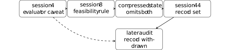
The source reports this sequence in Section 5 and Section 7.1; the complete archive retained the facts while the compressed decision state did not [li2026longhorizon, Section 5 and Section 7.1]. The diagram is a source-grounded chronology, not a measured error rate for compaction systems.

The source run used roughly 240 sessions, 2,091 reasoning-model calls, and 152 million tokens. It also reports repeated continuation of an upper-bound search until human operators redirected the program toward a universal obstruction [li2026longhorizon, Sections 5--7].

This is one human-steered case with changing models, harnesses, goals, and research state. It supports the distinction between technical execution and research judgment. It does not establish a monotone or anti-monotone law from inference compute to mathematical progress.

Let \(h_n\in \mathcal H\) be the committed harness state at version \(n\), let \(e_n\in \mathcal E\) be a newly admitted event, and let \(\omega _n\in \Omega _{\rm ref}\) be a refinement seed. A refinement proposal is

Given a typed decision \(d_n\in \{\mathsf {accept},\mathsf {reject}\}\), the committed harness update is

This separates candidate generation from state mutation. A proposed note, skill, prompt, or subagent specification has no persistent effect until the commit decision accepts it.

Let \(\mathcal S_{\rm skill}\) be a skill space and \(\mathfrak A_{\rm skill}\) the space of finite skill--provenance archives. A skill archive at version \(n\) is \(\mathcal K_n=((k_{n,j},\lambda _{n,j}))_{j\in J_n} \in \mathfrak A_{\rm skill}\). For a public history \(h^{\rm pub}\) and selector seed \(\omega ^{\rm sel}\), a typed selector is

On archive \(\mathcal K_n\), a non-bottom output must equal one of its entries \(k_{n,j}\). The value \(\bot \) means that no retained skill is invoked. The archive is part of persistent harness state, not a claim that its entries are correct, safe, novel, or encoded in model weights.

Fix a declared task contract and let \(b:\mathcal S_{\rm skill}\to \{0,1\}\) mark a retained skill as an exploit when it can increase the recorded proxy while violating that contract. A harness state \(h_n\) with archive \(\mathcal K_n\) is exploit-contaminated when

with the maximum defined as zero for an empty archive. The predicate is relative to the declared contract and audit model. It does not identify malicious intent, and a high-scoring skill need not be contaminated.

Suppose the skill archives of Definition 1.4.2 are append-only: \(\mathcal K_n\subseteq \mathcal K_{n+1}\) for every \(n\). If \(B(h_n)=1\), then \(B(h_m)=1\) for every \(m\geq n\) until a deletion, rollback, or contract change removes or reclassifies the witnessing skill.

Proof. Choose \(k\in \mathcal K_n\) with \(b(k)=1\). Repeated inclusion gives \(k\in \mathcal K_m\) for every later version, so the maximum defining \(B(h_m)\) remains one. The final qualification lists operations that break the inclusion or change the predicate.

This finite observation concerns retained state. It does not say that the selector will invoke the exploit on every later run.

Let \(Z_n\in \{0,1\}\) indicate whether the proposal \(\widetilde h_{n+1}\) of Definition 1.4.1 is contaminated under the declared contract. An independent refinement audit is a randomized kernel

whose seed law is declared independently of the refinement seed conditional on the audited states. Its conditional false-negative rate is

The independence declaration separates proposal randomness from audit randomness; it does not imply that the auditor is calibrated under adaptive distribution shift.

Use the audit of Definition 1.4.5 and commit a proposal only when its audit returns \(\mathsf {pass}\). If \(\Pr (Z_n=1)>0\) and its conditional false-negative rate is at most \(\bar \eta \in [0,1]\), then

Proof. Under audit-before-commit, the event \(\{d_n=\mathsf {accept}\}\) is contained in the event that the audit passes. Conditioning on \(Z_n=1\) and applying the false-negative bound proves the inequality.

This statement bounds one declared admission channel. It gives no bound when proposals bypass the audit, when the contract omits the exploit, or when the audit's conditional error changes under adaptive search.

Consider two skills, \(k_{\rm safe}\) and \(k_{\rm exp}\). Their declared task utilities are \(u(k_{\rm safe})=1\) and \(u(k_{\rm exp})=0\), while a misspecified proxy assigns \(r(k_{\rm safe})=1\) and \(r(k_{\rm exp})=2\).

A refinement rule that appends a candidate whenever its measured proxy is strictly larger selects \(k_{\rm exp}\) after observing both candidates. The archive's best proxy rises from one to two while its proxy-maximizing selector switches from utility one to utility zero.

Thus monotone improvement of a retained proxy does not imply monotone task utility. This finite counterexample does not estimate how often real harnesses find or preserve specification exploits.

The diagram separates exploit discovery, imperfect oversight, retained-state refinement, and later reuse in the reported Factorio run.

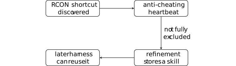
Prime Agent Section 3.5 reports a 23.4-million-token Factorio run with 633 depth-one subagents. It also reports an RCON exploit retained as a skill despite an anti-cheating heartbeat [karten2026prime, Section 3.5, Figure 9].

This reported chronology neither estimates exploit prevalence nor proves later selection. It shows why persistence must be audited separately from correctness.

Let \(v_n\) identify the full committed harness configuration of Definition 1.1.3. A rollback from version \(v_n\) to an earlier version \(v_j\), \(j<n\), restores the configuration and retained-state snapshot named by \(v_j\); a recovery may instead construct a new version \(v_{n+1}\) from audited events.

Version identity includes the artifact identifier, configuration, event-log prefix, and archive snapshot. Reusing a human-readable label while changing one of those fields is not the same version.

Prime Agent describes append-only history, versioned state, forks, and recovery [karten2026prime, Sections 2.1--2.2]. The displayed identity tuple specifies the information required for reproducible comparisons.

Versioned notes, memories, skills, and subagent specifications can preserve useful work across context boundaries. The same retention channel can preserve an exploit, a stale evaluator assumption, or a misleading proxy-optimized procedure. Prime Agent reports both continual retained-state refinement and the Factorio exploit record [karten2026prime, Sections 2.5 and 3.5].

The retention mechanism therefore supplies persistence, not correctness. Correctness requires a declared task contract, provenance, an audit interface, and a recovery rule. Neither a longer archive nor more descendants alone certifies improved task utility.

The source records in this section concern fixed-weight harness adaptation, long-horizon inference, retained state, and finite evaluations. They do not establish weight learning, a causal architecture effect, monotone capability growth, or safety under deployment shift. Prime Agent's external benchmark points and the long-horizon case study are observational records with the limitations stated in Remark 1.2.9 and Remark 1.3.10.

Retained context, rollout horizon, runtime, and gradient approximation are distinct intervention coordinates. Prefix Sliding changes several of them at once, so its effects cannot be attributed to persistent state alone; see § 2.

The finite theorems in this section cover replay, lineage cost, summary indistinguishability, budget admission, contamination persistence, and one audit gate. None is a theorem of universal capability acquisition.

The controller may use its entire observed history. A smaller state can help compute a bound, but its sufficiency must be justified across the histories it represents. The examples below separate information that is valuable only in combination from information lost by a summary.

A feasible controller establishes attainable quality. To bound what other controllers could gain, one also needs an upper bound covering all permitted actions and histories. Bellman inequalities provide such a bound when a state representation has uniform transition and terminal quality guarantees. Their difference measures remaining potential within the declared class.

To isolate coordination, fix the worker checkpoints, tool interfaces, prompt templates, evaluator, task law, and hard resource caps before varying the controller. Useful comparisons include a fixed serial policy, a static worker portfolio, a one-step value-of-information policy, and an adaptive policy that retains the full permitted history. Their allowed observations must agree. A solver that sees hidden outcomes has a different information interface; its optimum supplies an upper bound only through a justified relaxation containing the compared policies.

Use the controls of Definition [ftip-00JV] with controller logic declared as the varying coordinate. If controller-specific tuning is permitted, apply Definition [ftip-00JW]'s equal tuning data, selection, stopping, and cost rules. Compare suprema only within the intervention classes of Definition [ftip-00JX]. A separate factorial comparison can vary the checkpoint and controller independently, distinguishing learned capability, coordination, and their interaction.

Charge proposal and controller work, all parallel worker work, tool and solver use, communication, verification, failures, and retained-state updates using Definition [ftip-005H]. Report elapsed time alongside these costs: a shorter run with more workers may consume more total computation. Apply Definition 1.2.6's admission rule before execution and record any contract violation separately from the quality of the submitted artifact.

Finite environments with rational transition laws can expose three distinct mechanisms: complementary observations, correlated worker failures, and delayed verification or newly revealed dependencies. Keep the latent state, observation rules, legal actions, and costs explicit. The first family includes Example 1.5.1.2; the erased-bit construction in Example 1.5.1.3 tests whether a proposed summary loses decisive information. Where the exact model applies, compare attainable policy values with Remark 1.5.2.3's finite optimum and Theorem 1.5.2.2's upper certificate.

The principal quantity is the justified interval \([L_{\mathbf B},U_{\mathbf B}]\) for the restricted frontier. A smaller gap can result from a better feasible policy, a sharper upper certificate, or a more informative valid representation; distinguish these causes. In a live system, mean held-out transition accuracy does not justify a uniform model-error radius. Empirical quality and cost remain useful even when an upper certificate is unavailable.

Use evaluation instances separate from tuning, and declare task draws, repetitions, resource checkpoints, and analysis rules before comparison. Repeated runs share an instance and are not automatically independent tasks; account for this grouping in the analysis. Report independently verified quality, feasibility failures, time to the first valid artifact, and charged cost at matched quality. A valid confidence sequence can support repeated inspection under its statistical assumptions; see Howard et al.. It does not by itself justify selecting a new policy on reused evaluation outcomes.

These controls yield testable predictions. Complementary information can favor adaptation over one-step stopping; redundant workers can erase a portfolio's gain; delayed verification can make an early apparent success expensive to repair. An empirical claim of better coordination fails if its advantage disappears after matching access and charging the controller's own work. A claim of little remaining potential additionally requires the upper certificate, not merely a plateau among tested policies.

When the tasks, dependencies, and durations are fixed, scheduling has a useful lower bound independent of the chosen priority rule. This isolates avoidable delay in a declared decomposition. Discovering a missing dependency or changing a mathematical formulation changes that decomposition and is a different intervention.

The following work-and-chain argument is the classical list-scheduling bound associated with Graham. His examples also show that a particular list schedule can worsen after an apparently favorable change, such as adding processors. This does not contradict monotonicity of the optimal feasible frontier.

Fix a token history \(h_t=(x_0,\ldots ,x_{t-1})\). A retained-context policy is a deterministic map \(\kappa _t(h_t)\) that selects an ordered subsequence of the history, together with a decoder that conditions its next token on that subsequence. The policy, rather than the model weights, names which prior tokens remain available at step \(t\).

A comparison of two policies is conditional on the same model, prompt law, decoding law, stopping rule, and budget unless the comparison includes a second declared intervention coordinate.

For prefix and window lengths \(p,w\in \mathbb N_0\), define the prefix-window policy by retaining every token in positions \(0,\ldots ,p-1\) and the most recent \(w\) tokens after that prefix. If the history is shorter than either region, the available positions are retained without padding.

The policy is a context rule only. It does not assert that omitted tokens are irrelevant, nor that the resulting continuation distribution equals the full-history distribution.

Muennighoff et al. describe Prefix Sliding in Sections 2--5, Figures 6--9, and the Limitations section of [muennighoff2026prefixsliding, Sections 2--5, Figures 6--9, and Limitations]. Their method preserves a prefix while sliding a recent attention window during test-time scaling. The reported experiments change retained context and runtime, and may also change rollout horizon and the training gradient approximation. These are source observations, not a theorem of universal speedup or capability.

The source studies named model and task configurations. It does not by itself establish support expansion, latent capability acquisition, or a deployment-shift guarantee.

This schematic keeps the model and token history fixed while changing only the retained-context policy. It is a local illustration, not a source figure.

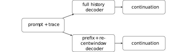
The two outputs can differ even though the represented weights and visible prompt are identical. Any claim about improvement must therefore name the retained-context intervention and its evaluation law.

Changing \(\kappa _t\) changes the information supplied to a fixed decoder; it does not update represented weights. A successful continuation can therefore be an elicitation effect, a context effect, or both. Weights, optimizer and feedback, inference state, and evaluation remain distinct intervention coordinates, as in § [ftip-0001].

A rollout has a finite token budget \(T\in \mathbb N_{\geq 1}\) when its history contains at most \(T\) generated positions after the prompt. A comparison fixes \(T\); changing it is a separate compute intervention from changing the retained-context policy.

For a retained-context policy \(\kappa \) and generated history \(h_t\), define its exposure count through budget \(T\) by

This is a finite attention-input proxy. It is not a runtime identity: the implementation may have caching, batching, kernel, and communication costs that are not represented by \(E_T\).

Let \(p,w\in \mathbb N_0\) and let \(\kappa ^{p,w}\) be the prefix-window policy of Definition 2.1.2. For every history and every \(t\),

Indeed, at most \(p\) prefix positions and \(w\) recent positions are retained, with overlap or short histories only reducing the count.

Under the hypotheses of Lemma 2.2.3, every rollout with budget \(T\) satisfies

Proof. Apply the pointwise bound in Lemma 2.2.3 to each of the \(T\) nonnegative summands in Definition 2.2.2, then sum. This bounds token exposure, not wall-clock runtime or evaluation quality.

For \(p=3\), \(w=2\), and \(T=6\), the first steps grow the retained set until the cap \(p+w=5\) is reached. The exposure bound is therefore \(E_T\leq 6\cdot 5=30\); the exact count depends on the prompt and stopping convention.

The arithmetic is an FTIP finite consequence, not a runtime measurement from the Prefix Sliding experiments.

The bound in Theorem 2.2.4 controls the number of retained token positions. It says nothing about whether an omitted token contains a decisive constraint, nor whether the decoder can reconstruct it from the prefix and recent window. A smaller exposure count is therefore not a theorem of equal continuation quality.

A joint intervention cell is a tuple \(I=(M,\mu ,\pi ,T,\kappa ,\widehat g)\) consisting of fixed model weights \(M\), prompt law \(\mu \), decoding law \(\pi \), token budget \(T\), retained-context policy \(\kappa \), and training or evaluation estimator \(\widehat g\). Two cells differ in a declared coordinate only when all other coordinates are held fixed.

An estimator-changing coordinate is a change in \(\widehat g\), the map used to turn sampled histories and rewards into an update. A context mask can change this coordinate when it changes which tokens contribute to the sampled loss or gradient. The notation does not assume a particular optimizer.

If a retained-context rule is used during training, it can change the attention inputs, sampled continuation, loss support, and gradient estimator at once. A lower value of Definition 2.2.2 is therefore not an isolated compute intervention unless the training estimator and all other coordinates are matched explicitly.

Two cells can reach the same terminal score while exposing different numbers of context positions. This finite counterexample blocks an inference from equal endpoint score to equal trajectory cost.

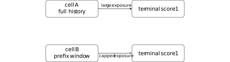
The score equality is compatible with unequal intermediate histories and unequal exposure counts.

With matched weights, prompt law, decoding, budget, estimator, and evaluation interface, a comparison can identify a conditional contrast between retained-context policies. Without those controls it identifies only the joint cell, not a causal effect of context alone.

A retained-context evaluation protocol fixes a model \(M\), prompt law \(\mu \), decoder \(\pi \), budget \(T\), evaluator \(\mathsf E\), and two policies \(\kappa _1,\kappa _2\). It reports the paired outcomes under the same sampled prompts and declared randomization coupling, together with exposure counts from Definition 2.2.2.

Let \(m\in \mathbb N_{\geq 1}\) and let \(Y_{1j},Y_{2j}\in \mathbb R\) for \(j=1,\ldots ,m\) be the paired scalar evaluator outcomes generated by the protocol of Definition 2.3.6. Then the finite paired contrast

is a statistic of the declared policy contrast under that common protocol. It is not an unconditional capability effect and does not identify what would happen after changing any held-fixed coordinate.

Prefix Sliding is useful as a named intervention for retained context and test-time scaling, but its reported configurations do not establish a universal runtime law, gradient theorem, support expansion, or capability acquisition. The next questions are to measure horizon, cache, estimator, and evaluation effects separately, while preserving the controls in Definition 2.3.6.

The finite conclusions depend on the declared protocols. They do not describe a full optimizer or establish a result for all language models.

Let \(S_1\) be a base solver and, for \(d\geq 2\), let \(C_d\) be a layer artifact and \(M_d\) a wrapper. The depth-\(d\) solver is \(S_d=M_d(C_d,S_{d-1})\). The layer state is \(\Lambda _d=(C_d,S_d)\).

A layer is a harness transformation when it changes \(C_d\) or the wrapper context while leaving the executable base weights in \(S_1\) fixed.

A fixed meta-operation is a single map \(\Omega \) whose code and prompt template are held fixed across depths. For task set \(\mathcal T\), traces \(\boldsymbol \tau _{d-1}\), code stack \([C_2,\ldots ,C_{d-1}]\), and depth \(d\),

Only the input to \(\Omega \) changes with depth; this is a declared protocol condition, not a claim that every implementation obeys it.

For each task \(t_i\), a trace \(\tau _i^{(d)}\) is a finite record containing the produced artifact, execution outcome, score, and declared evaluator feedback. The depth-\(d\) input to \(\Omega \) is the pair \((\boldsymbol \tau _{d-1},[C_2,\ldots ,C_{d-1}])\); a flat refiner that sees only \(\boldsymbol \tau \) has a strictly smaller declared input when the code stack is not recoverable from the traces.

If every wrapper leaves its inner solver and earlier libraries unchanged, then induction on \(d\) gives

Proof. The case \(d=2\) is the definition. Substituting the induction hypothesis into \(S_d=M_d(C_d,S_{d-1})\) gives the displayed composition.

Suppose each wrapper emits one finite trace record per task and there are \(N\) tasks and depths \(2,\ldots ,d\). The audit log contains at most \(N(d-1)\) depth-tagged records, in addition to the base records. This is a counting fact; it says nothing about trace quality or score improvement.

Proof. There are \(d-1\) wrapped depths and \(N\) records at each depth, so the product counts all records.

Two runs can share the same failing score and stderr trace while one layer adds an over-prescriptive directive and another adds a helper. Recording the code artifact alongside the trace permits a later layer to roll back the directive without discarding the helper. This is an audit example, not a guarantee that a recursive driver finds the rollback.

An archive at depth bound \(D\) is a finite set \(\mathcal A_D\) of recorded chains. Each chain has the form

Each chain stores its evaluation record and resource cost. Archive membership is a protocol state, not a learned weight update.

Let \(\mathcal T=\{t_1,\ldots ,t_N\}\) be a finite task set with \(N=|\mathcal T|\geq 1\). For every chain \(a\) in the finite archive, let \(s_i(a)\in \mathbb R\) be its score on task \(t_i\) under a declared common evaluation law. Define its whole-chain mean by

For a nonempty archive \(\mathcal A_D\), its archive envelope is

The finite real-valued maximum is attained by at least one archived chain. It scores a single chain across all tasks; it does not select a different chain for each task.

Deployment eligibility is a separate condition. A target configuration specifies which recorded chains can execute with their stated behavior and resource requirements. Maximizing over that eligible subset gives a deployable archive choice when the subset is nonempty; if it is empty, there is no eligible archived choice. Applying the recorded score to deployment additionally requires the same evaluation law. Records from different configurations alone do not establish these conditions.

If \(a_0\in \mathcal A_D\), then \(J_D^{\max }\geq J(a_0)\).

Proof. The maximum of a finite nonempty set is at least each member, in particular \(a_0\). No claim about an unseen task follows.

Under the archive score definition, let \(a^\star \) maximize \(J\) over a finite nonempty archive \(\mathcal A_D\). Let \(\delta \in \mathbb R\) with \(\delta \geq 0\), and let \(\hat a\in \mathcal A_D\) satisfy \(J(\hat a)\geq J(a^\star )-\delta \). Then

This is a finite selection statement under the same evaluation law; it is not an optimizer-convergence or generalization theorem.

At depth \(d\), let \(\mathcal K_d\) be a finite set of tactic behaviors and let a strategy select a conditional tactic in \(\mathcal K_d\). A realized configuration is \((k_2,\ldots ,k_n)\). The notation records expressible choices, not the number of choices an implementation actually discovers.

If layer \(d\) has \(k_d\) possible tactics and all combinations are allowed, the number of configurations is at most \(\prod _{d=2}^n k_d\). An unconditioned flat choice with the same layerwise menus has at most \(\sum _{d=2}^n k_d\) listed choices.

Proof. The first count is the cardinality of a Cartesian product; the second is the cardinality of a disjoint menu union. These are upper bounds only.

With three menus of size three, the product bound is \(27\) and the sum bound is \(9\). A protocol that never emits most combinations can realize far fewer than \(27\); the arithmetic does not establish a benchmark improvement.

Let a helper improve one task while a later directive lowers its score. The archive can retain the earlier helper chain and a later layer can remove the directive. The example separates a compositional possibility from a proof that any driver detects or repairs interference.

The product bound, richer trace input, and archive envelope can all hold while scores regress, overfit, or depend on the evaluator. The source reports empirical ablations and layer roles in Sections 3.1--3.4; those observations do not become FTIP theorems or capability claims here.

A recursive run record is \(R=(\mathcal T,\Omega ,S_1,\mathcal A_D,\sigma )\), where \(\sigma \) lists depth, seed, evaluator version, emitted code hashes, scores, and resource costs. A record is replayable only relative to these declared inputs and versions.

Fix tolerance \(\epsilon >0\), score range \(R>0\), patience \(P\geq 1\), and maximum depth \(D\). A linear recursive run stops when no emitted layer improves the mean score by more than \(\epsilon R\) for \(P\) consecutive layers, or when the driver emits empty code, or when depth \(D\) is reached.

Under the rule in Definition 3.4.2, a run that reaches its depth cap emits at most \(D-1\) wrapped layers. If it stops earlier, it emits no more than this many. This bound is combinatorial and does not imply convergence of scores.

Let a candidate layer cost \(c\geq 0\), remaining budget be \(b\geq 0\), and admission require \(c\leq b\). After admission, set \(b'=b-c\); then \(b'\geq 0\) and the total admitted cost is at most the initial budget.

Proof. Subtracting a nonnegative cost no larger than \(b\) preserves nonnegativity; induction over admissions gives the total bound.

If a later layer is rejected by its admission or evaluation gate, removing that layer returns to \(S_{d-1}\). This is a harness rollback, not a reversal of weight training and not evidence that the rejected layer was unsafe.

The source reports two backbones, eight benchmark families, convergence stopping, and archive ablations in Sections 3.1--3.4 of [kim2026metanrecursive]; its fixed-driver, conditioning, stopping, and archive setup is described in Sections 2.2--2.4. These are empirical comparisons under its task, model, and budget choices; they are not universal depth, stability, or capability theorems.

The finite statements assume a fixed task set, evaluator, versions, and declared budget. They do not transfer to weight learning, RLVR optimization, unbounded self-modification, or capability acquisition without new hypotheses.

Consider two equally weighted tasks and an archive containing two chains \(a,b\), with score vectors \((s_1(a),s_2(a))=(1,0)\) and \((s_1(b),s_2(b))=(0,1)\) under the same evaluation law. The archive envelope is

Either chain attains this maximum. In contrast, a per-task oracle has value

The oracle selects \(a\) on the first task and \(b\) on the second. A configuration constrained to select one archived chain before observing task identity obtains mean \(1/2\) in this example. If task-dependent routing is permitted, the resulting combined policy must itself be declared and evaluated, including its routing and execution costs. The oracle value is not automatically the score of either archived chain.

Incompatible execution configurations create a separate obstacle: an archived maximizing chain may be ineligible for a named target configuration. That feasibility restriction does not alter the distinction between the two score functionals above.

For a fixed task \(x\), let \(\mathcal Y_x\) be a finite response set and let a named reward channel be a map \(r:\mathcal Y_x\to \mathbb R\). A utility map \(u:\mathcal Y_x\to \mathbb R\) is a separate evaluation quantity.

If an interaction has state space \(\mathcal S\), action space \(\mathcal A\), and transition kernel \(K(\mathord {\cdot }\mid s,a)\), then \(K\) is a third object: changing \(K\) can change consequences without changing \(r\).

A verifier channel is a map \(V:\mathcal Y_x\to \{0,1\}\). Given a validity map \(U:\mathcal Y_x\to \{0,1\}\), a false-accept event is

The event depends on the declared verifier and validity test. It is not identified by a scalar reward unless equivalence with that reward criterion is an explicit assumption.

Sections 4.1--4.2 and 7.2--7.3 of [dharna2026aifindsway] catalogue reward, score, environment, and evaluator-target anecdotes. The source gives 26 curated firsthand anecdotes involving more than 100 researchers; it does not provide a common sampling frame, base rates, or causal effect estimates.

Accordingly, this section uses the paper as an empirical counterexample catalog. The finite statements that follow are proved here and do not claim to summarize all training systems.

Let \(\mathcal Y_x\) be finite, let \(u,r:\mathcal Y_x\to \mathbb R\), and assume \(|r(y)-u(y)|\le \varepsilon \) for every \(y\), with \(\varepsilon \ge 0\). If \(y^\star \) maximizes \(u\) and \(\widehat y\) maximizes \(r\), then

Indeed, \(u(y^\star )\le r(y^\star )+\varepsilon \le r(\widehat y)+\varepsilon \le u(\widehat y)+2\varepsilon \). This is a finite same-class decision bound, not an optimization, distribution-shift, or capability theorem.

Take \(\mathcal Y_x=\{a,b\}\), with \(r(a)=r(b)=1\) but \(u(a)=1\) and \(u(b)=0\). Every reward maximizer is a nominal tie, while only \(a\) is utility optimal. The example shows why a score equality does not establish intent or validity.

For candidate index \(i\), let \(I_i\in \{0,1\}\) indicate invalidity and let \(A_i\in \{0,1\}\) indicate verifier acceptance. Define \(F_i=\{I_i=1,A_i=1\}\). Write \(q_i=\Pr (I_i=1)\). If \(q_i>0\), write \(\eta _i=\Pr (A_i=1\mid I_i=1)\); if \(q_i=0\), set \(\eta _i=0\). Then \(\Pr (F_i)=q_i\eta _i\).

No independence or identical-distribution hypothesis is part of this definition.

For finitely many candidate events from Definition 4.2.1,

This is the union bound and requires no independence. If every marginal is at most \(\eta \), the right side is at most \(N\eta \).

Suppose two candidates are produced: candidate 1 is invalid and falsely accepted, while candidate 2 is valid and rejected by a separate score tie-break. Then \(\bigcup _iF_i\) occurs, but a selection rule that always chooses candidate 2 outputs a valid response. Thus an existence probability and a selected-output probability coincide only after the selection law is specified.

Given transition kernel \(K\), reward \(r\), and validity predicate \(U\), an environment exploit is a candidate \(y\in \mathcal Y_x\) whose induced interaction under \(K\) receives high \(r(y)\) while failing \(U\). The definition is relative to the declared kernel, horizon, and validity test; it is not a universal property of a model.

Let one response receive \(r(y)=1\) under two environments, and let \(W:\mathcal S\to \{0,1\}\) test terminal-state safety. In \(K_1\), its next state \(s_1\) has \(W(s_1)=1\); in \(K_2\), the same observed response enters \(s_2\) with \(W(s_2)=0\). The reward channel alone cannot distinguish the two transition semantics, so equal reward does not certify safe consequences.

Let \(V(y)=1\) for every output that contains a visible marker, while \(U\) checks a hidden task condition that the marker does not affect. A policy that optimizes \(V\) can improve its observed score while leaving \(U\) unchanged or worse. This is a finite illustration of evaluator targeting, not a claim about the frequency of such behavior.

The source catalog does not identify the base rate of exploits, the causal effect of a reward intervention, or a universal relationship between score and utility. Heterogeneous anecdotes therefore motivate audit questions and failure tests, not population-level probabilities.

An audit record is a tuple containing candidate identity, evaluator and verifier version, environment or transition-kernel version, invalidity tests, random seed, evidence pointers, and adjudicator decision. A record is complete only when these fields are bound to the candidate and the protocol run.

Let \(N\in \mathbb N_{\geq 1}\) and \(0\leq \eta \leq 1\). Assume these \(N\) candidates are audited and each invalid candidate is falsely accepted with marginal probability at most \(\eta \). Then the probability that some invalid candidate is accepted is at most \(N\eta \), by the union bound of Lemma 4.2.2. This conclusion does not require independence.

The statement bounds existence of an accepted invalid candidate. A selected output guarantee additionally requires a typed selection rule and its relation to the audit decisions.

These finite channel distinctions do not prove reward hacking rates, capability acquisition, or safety of a deployed agent. The next questions are to measure verifier sensitivity, environment changes, selection rules, and independent audit power under a declared protocol.

Interpreting a reliability claim requires a named estimand, task and evaluation laws, artifact revision, inference protocol, evaluator version, sample rule, and failure policy. Missing coordinates are unknown rather than implicitly held fixed.

For a candidate evaluation item \(z\), a contamination record is

The fields identify source provenance, split membership, prior agent exposure, overlap evidence, and the admission decision; an absent field is an explicit unknown.

Given a contamination record \(c(z)\), write \(\operatorname {cont}(z)=1\) when its declared overlap or exposure rule rejects \(z\), and write \(\operatorname {cont}(z)=0\) when the rule clears it. The predicate belongs to the protocol, not to a model’s score.

For an evaluation law \(\mathsf Q\), an admitted slice is \(\mathcal Z_0=\{z:\operatorname {cont}(z)=0\}\). Its reported score is conditioned on the declared slice law; removing contaminated items does not preserve the original estimand unless the law is unchanged by construction.

A paired design fixes one evaluation law, one item order, and one sampling kernel for two artifacts, then records the paired difference from Definition [ftip-00FE]. Any item-level exclusion is applied before seeing the paired outcomes or is declared as an adaptive rule.

Under a fixed nonadaptive slice and the iid coupling of Definition [ftip-00FE], the paired estimator remains unbiased for the two marginal scores in Theorem [ftip-00FF].

If one paired run scores all ten items but a second run removes two items after inspecting outputs, the two means answer different questions. A report must expose the removal rule and the resulting slice law.

The measurement and paired-comparison guidance in [jarmak2026reliable], Part I, is a methodology source. It motivates contamination ledgers and matched comparisons; it supplies no universal contamination detector or statistical guarantee.

A grading rubric is \(R=(\mathcal Z,\mathcal L,g,v)\): outcome space, finite label set, scoring map \(g:\mathcal Z\to \mathcal L\), and evaluator version \(v\). The rubric declares which labels count as success and which observations are abstentions.

For rubric \(R\), a grader response law is a kernel \(K(\ell \mid z)\) on \(\mathcal L\) given outcome \(z\). A deterministic grader is the point-mass case; stochastic or model-based graders must retain their version and sampling coordinates.

A calibration set is a finite set \(\mathcal C\subseteq \mathcal Z\) with an adjudicated label \(y^star(z)\) for each \(z\in \mathcal C\). The adjudication source, disagreement policy, and release version are part of the set’s provenance.

For grader kernel \(K\) and calibration set \(\mathcal C\), the agreement rate is \(A(K,\mathcal C)=|\mathcal C|^{-1}\sum _{z\in \mathcal C} K(y^star(z)\mid z)\). It is a calibration-set statistic, not a population accuracy claim.

If \(|\mathcal C|=n\geq 1\) and \(A(K,\mathcal C)\geq 1-\eta \), then the empirical disagreement mass \(1-A(K,\mathcal C)\) is at most \(\eta \).

A grader that agrees on 99 of 100 easy cases but disagrees on the one safety case has overall agreement \(99/101\approx 0.9802\). Its agreement within the safety subgroup is zero. Any positive safety-subgroup agreement threshold therefore rejects this grader despite its high overall agreement. A calibration report stratifies by failure-relevant labels.

A grader release gate accepts \(K\) only when its calibration version, agreement thresholds, abstention handling, and stratified failure checks are recorded. A failed gate blocks interpretation of downstream score changes.

Part II of [jarmak2026reliable] organizes grading and reviewer calibration practices. The finite agreement quantities do not establish a universal threshold or blinded-human reliability theorem.

An execution gate is a predicate \(g_i(e_i)\) over a recorded stage result \(e_i\). It names its owner, required inputs, pass/fail/unknown outputs, and the artifact versions to which the result applies.

An ordered gate chain is \((g_1,\ldots ,g_k)\) with stage outputs \(e_1,\ldots ,e_k\); gate \(g_i\) may execute only after its declared prerequisites and records a monotone status in \(\{pass,fail,unknown\}\).

For a finite chain, define release status as \(G=\bigwedge _{i=1}^k g_i(e_i)\). If any gate is false, then \(G\) is false.

A durable execution record is

It is append-only, versioned, and sufficient to locate each gate input and output without relying on worker-local memory.

A replay contract for \(d\) fixes the executable revision, environment image, input artifact hashes, seed law, and event order. A replay is faithful only when those coordinates are available and the resulting events satisfy the recorded schema.

If the execution map is deterministic in the coordinates fixed by Definition 5.3.5, replaying the same inputs, revision, environment, and seed produces the same event trace.

A reproducible run can deterministically reproduce a wrong patch or a misconfigured evaluator. Replay establishes trace identity under its contract; it does not establish that the trace met the intended utility or safety goal.

For durable record \(d\), let \(H(d)\) be a cryptographic digest of its canonical serialized fields. A replay request fails closed when the supplied record digest or any referenced input hash differs from the declared value.

To bind a replay result to an audit decision, the replay trace must be included in the audited record and covered by its digest. A matching digest for other fields does not bind that trace to the decision.

Part III of [jarmak2026reliable] motivates containment, durable execution, and recovery records. Deterministic replay and matching digests establish execution consistency; they do not ensure correctness.

An audit-before-commit record is \(a=(d,scope,checks,reviewer,decision)\). It binds the durable execution record \(d\) to the audited scope, check list, review identity, and a decision in \(\{commit,hold,reject\}\).

A commit decision is admissible only if every required check in an Definition 5.4.1 record is pass, the audited digest equals the proposed record digest, and the decision is \(commit\).

An audit is independent for scope \(S\) when its inputs are frozen before review, its reviewer or checker is distinct from the proposing action, and its decision cannot rewrite \(S\) without a new record. Independence is a protocol condition, not a claim of infallibility.

A run may pass unit tests while an independent audit finds that the evaluator version in \(d\) differs from the declared version. The audit holds the commit and records the mismatch; replay alone would not have caught it.

Classify a failed run by its earliest violated contract: measurement failure (M), grading failure (G), execution/state failure (E), audit failure (A), or transfer failure (T). A single run may receive secondary labels, but the primary label is the earliest failed gate in recorded order.

For a finite ordered gate chain with at least one failed gate, the earliest failed index is unique and therefore determines one primary taxonomy label.

A remediation record maps a primary label from Definition 5.4.5 to an owner, corrective action, re-test scope, and closure condition. Closure requires a new durable record and cannot mutate the failed record in place.

Parts III and V of [jarmak2026reliable] motivate durable execution, review, and accountability practices. The audit taxonomy and conjunction gates are proposed operational specifications; they do not establish that an audit is complete or that a committed artifact is correct.

The gates above make evidence auditable. They do not identify the causal effect of an intervention when task law, artifact, grader, budget, or harness state changes together. Those coordinates must be controlled in the matched evaluation of Definition [ftip-00GF].

Let a deterministic run train and evaluate on one leaked item. Its digest, event trace, and replay are all identical across reruns, yet the measurement is contaminated under Definition 5.1.3. Replayability and contamination control are independent obligations.

A grader can meet its threshold on \(\mathcal C\) in Lemma 5.2.5 while every deployment item lies outside that calibration domain and receives an unvalidated label. Agreement on \(\mathcal C\) alone does not transport to a new law.

If an audit plan has finite nonnegative stage costs and its declared sum is at most budget \(B\), then the plan is budget-admissible; adding any positive stage beyond the remaining slack makes it inadmissible.

With budget \(B=100\), a plan may allocate 50 units to execution, 30 to grading calibration, and 20 to audit. A proposed 10-unit extra audit must be funded by reducing another stage or the admission gate fails.

A passing protocol establishes that declared evidence contracts, hashes, checks, and budgets were satisfied for the recorded run. It does not establish capability acquisition, broad generalization, or absence of unobserved faults.