Alignment gain and preference information [ftip-008E]
✍️sourceAGENTDRAFTED
Alignment gain and preference information [ftip-008E]
✍️sourceAGENTDRAFTED
Two finite models ask different questions about post-training. The first assumes an exact KL-regularized optimizer and characterizes the reward gain that its exponential tilt can produce. The second asks what ordinal comparisons reveal when post-training may reroute a fixed set of response circuits.
Neither source model is a general account of neural post-training. The first assumes exact optimization of a declared scalar reward. The second is a stylized routing model with a fixed circuit set. Extending the KL identity to an approximate optimizer requires further analysis. Extending the ordinal routing conclusion to a changing circuit set requires additional assumptions on that change.
1. Finite KL-regularized alignment [ftip-008F]AGENTDRAFTED
1. Finite KL-regularized alignment [ftip-008F]AGENTDRAFTED
This subsection studies an exact, finite optimization model. A reference law is exponentially tilted by a declared scalar reward. In this setting, reward gain admits two exact descriptions: a Jeffreys-divergence identity and a covariance under the reference law.
The statements do not model approximate optimization, neural training cost, reward validity, or independent capability evaluation.
Remark 1.1. Exact optimization on a finite response set [ftip-008G]AGENTDRAFTED
Remark 1.1. Exact optimization on a finite response set [ftip-008G]AGENTDRAFTED
Theorems 1 and 2 of the v1 preprint [paes2026theoretical] concern an exactly optimal KL-regularized policy and a fixed query. On a finite response set, their expectations and normalizers are ordinary finite sums.
These exact identities do not establish a comparison among best-of-\(N\), PPO, and GRPO, or a general guarantee for proxy rewards and reward ensembles. Those questions require assumptions beyond exact optimization of one reward.
Notation 1.2. Translating the alignment source notation [ftip-008H]AGENTDRAFTED
Notation 1.2. Translating the alignment source notation [ftip-008H]AGENTDRAFTED
The source writes \(\lambda >0\) for the KL penalty. Here we write \(\beta >0\), matching the DPO notation in Notation [ftip-003M]--Definition [ftip-003O]. This avoids collision with the generalized-advantage parameter in Definition [ftip-003E] and the protocol law in Definition [ftip-007Q].
The source's gain \(\Delta (r,r')\) is written \(G_p(r;s)\): \(r\) is the reward used to tilt the reference law \(p\), while \(s\) is the reward used to evaluate the tilted law. This avoids collision with both the simplex notation \(\Delta (X)\) of Notation [ftip-000A] and the paired DPO margin of Notation [ftip-003M]. For a finite set \(\mathcal Y\), a law \(p\in \Delta (\mathcal Y)\), and functions \(f,g:\mathcal Y\to \mathbb R\), set
\[ \operatorname {Cov}_p(f,g) =\mathbb E_{y\sim p}[f(y)g(y)] -\mathbb E_{y\sim p}[f(y)]\, \mathbb E_{y\sim p}[g(y)]. \]
Definition 1.3. Finite KL-alignment instance [ftip-008I]AGENTDRAFTED
Definition 1.3. Finite KL-alignment instance [ftip-008I]AGENTDRAFTED
A finite KL-alignment instance consists of a nonempty finite response set \(\mathcal Y\), a reference law \(p\in \Delta (\mathcal Y)\), a penalty \(\beta >0\), and finite real functions \(r,s:\mathcal Y\to \mathbb R\). The reference support is
\[ S_p=\{y\in \mathcal Y:p(y)>0\}. \]A prompt is fixed and suppressed. The function \(r\) determines the alignment update; \(s\) measures its result. They may coincide, but they need not. Finiteness makes every exponential weight and expectation below finite.
These objects specialize the fixed-query setting in [paes2026theoretical, Section 2, equations (2.1)--(2.2)]; they are not a definition of alignment in general.
Definition 1.4. Exponential weight and partition function [ftip-008J]AGENTDRAFTED
Definition 1.4. Exponential weight and partition function [ftip-008J]AGENTDRAFTED
For a finite KL-alignment instance, define the exponential weight and partition function by
\[ a_r(y)=\exp \left (\frac {r(y)}{\beta }\right ), \qquad Z_r=\mathbb E_{y\sim p}[a_r(y)]. \]Every \(a_r(y)\) is finite and strictly positive. Since \(p\) is a probability law on a nonempty finite set, \(0<Z_r<\infty \).
This weight and normalizer are the fixed-query form of [paes2026theoretical, Equation (2.2)].
Definition 1.5. Aligned law in finite-source notation [ftip-008K]AGENTDRAFTED
Definition 1.5. Aligned law in finite-source notation [ftip-008K]AGENTDRAFTED
The aligned law induced by \(r\) is \(q_r\in \Delta (\mathcal Y)\) given by
\[ q_r(y)=\frac {p(y)a_r(y)}{Z_r}. \]Normalization follows from the definition of \(Z_r\). Moreover, \(q_r(y)>0\) exactly when \(p(y)>0\). This is the finite notation for the same exponential-tilt optimizer stated in Definition [ftip-003O]; support preservation was proved in Theorem [ftip-007C].
This formula is [paes2026theoretical, Equation (2.2)]. It assumes the exact optimizer, not an iterate returned by a particular training algorithm.
Definition 1.6. Cross-reward gain under an alignment reward [ftip-008L]AGENTDRAFTED
Definition 1.6. Cross-reward gain under an alignment reward [ftip-008L]AGENTDRAFTED
The cross-reward gain from aligning with \(r\) and evaluating with \(s\) is
\[ G_p(r;s) =\mathbb E_{y\sim q_r}[s(y)] -\mathbb E_{y\sim p}[s(y)]. \]The semicolon records two roles. Its left argument changes the response law; its right argument scores both laws. Thus \(G_p(r;s)\) is not an independent evaluation unless \(s\) has separately been declared to serve that role.
This is the finite notation for \(\Delta (r,r')\) in Theorem 2, equation (3.4), of Theoretical limits of language model alignment[paes2026theoretical].
Definition 1.7. Jeffreys divergence [ftip-008M]AGENTDRAFTED
Definition 1.7. Jeffreys divergence [ftip-008M]AGENTDRAFTED
For probability laws \(p\) and \(q\) for which both terms are finite, their Jeffreys divergence is
\[ J(p,q) =D_{\mathrm {KL}}(p\Vert q) +D_{\mathrm {KL}}(q\Vert p). \]The KL divergence and its argument order are defined in Definition [ftip-006X]. Unlike either directed term, \(J(p,q)=J(q,p)\). In the finite tilt of Definition 1.5, \(p\) and \(q_r\) have the same support, so both terms are finite.
Lemma 1.8. Log-density ratio of the exact tilt [ftip-008N]AGENTDRAFTED
Lemma 1.8. Log-density ratio of the exact tilt [ftip-008N]AGENTDRAFTED
For every \(y\in S_p\), the aligned law satisfies
\[ \log \frac {q_r(y)}{p(y)} =\frac {r(y)}{\beta }-\log Z_r. \]
Proof.
Proof.
On \(S_p\), both \(p(y)\) and \(q_r(y)\) are positive. Dividing the formula of Definition 1.5 by \(p(y)\) and taking logarithms gives the identity.
This is equation (B.1) followed by the logarithmic step in [paes2026theoretical, Appendix B.1, equations (B.1)--(B.2)].
Theorem 1.9. Exact reward gain equals scaled Jeffreys divergence [ftip-008O]AGENTDRAFTED
Theorem 1.9. Exact reward gain equals scaled Jeffreys divergence [ftip-008O]AGENTDRAFTED
For a finite KL-alignment instance,
\[ G_p(r;r)=\beta J(p,q_r). \]
Proof.
Proof.
Rearranging Lemma 1.8 gives \(r(y)=\beta \log (q_r(y)/p(y))+\beta \log Z_r\) on the common support. Taking expectation first under \(q_r\) and then under \(p\) yields
\[ \begin {aligned} \mathbb E_{q_r}[r] &=\beta D_{\mathrm {KL}}(q_r\Vert p)+\beta \log Z_r,\\ \mathbb E_p[r] &=-\beta D_{\mathrm {KL}}(p\Vert q_r)+\beta \log Z_r. \end {aligned} \]Subtracting cancels the common normalizer and gives the result.
This is the finite form of [paes2026theoretical, Theorem 1, equation (3.2), with proof in Appendix B.1].
Remark 1.10. What the Jeffreys identity does and does not identify [ftip-008P]AGENTDRAFTED
Remark 1.10. What the Jeffreys identity does and does not identify [ftip-008P]AGENTDRAFTED
The identity Theorem 1.9 is an equality inside one declared model. It says that exact gain in the optimizing reward equals a symmetric divergence from the reference law. It does not say that a larger divergence improves a different utility, nor that a training algorithm reaches the exact tilt.
The identity accounts for neither rollout and update work nor the cost of obtaining \(r\). Consequently it is not, by itself, a bound on the costed post-training potential of Definition [ftip-005M].
Theorem 1.11. Cross-reward gain is a base-law covariance [ftip-008Q]AGENTDRAFTED
Theorem 1.11. Cross-reward gain is a base-law covariance [ftip-008Q]AGENTDRAFTED
For a finite KL-alignment instance,
\[ G_p(r;s) =\operatorname {Cov}_p\left (s,\frac {a_r}{Z_r}\right ). \]
Proof.
Proof.
The aligned expectation can be written under the reference law as \(\mathbb E_{q_r}[s]=\mathbb E_p[s a_r/Z_r]\). Also \(\mathbb E_p[a_r/Z_r]=1\). Substituting these two identities into Definition 1.6 gives the covariance defined in Notation 1.2.
This is the finite form of Theorem 2, equation (3.4), in Theoretical limits of language model alignment[paes2026theoretical]. Its proof is in Appendix B.1, equations (B.5)--(B.7).
Remark 1.12. The covariance is predictive only for a declared reward [ftip-008R]AGENTDRAFTED
Remark 1.12. The covariance is predictive only for a declared reward [ftip-008R]AGENTDRAFTED
The identity Theorem 1.11 expresses exact tilted-law gain using expectations under \(p\). This makes the population quantity accessible from the reference law in principle. A finite-sample estimator still needs its own sampling law, moment assumptions, and error analysis.
The formula also remains indexed by both \(r\) and \(s\). It cannot turn a proxy reward into an independent utility. If \(s=r\), it measures improvement in the same quantity that defined the exact optimizer; if \(s\ne r\), its sign is determined by the displayed covariance.
Example 1.13. A two-response alignment identity [ftip-008S]AGENTDRAFTED
Example 1.13. A two-response alignment identity [ftip-008S]AGENTDRAFTED
Take \(\mathcal Y=\{a,b\}\), \(p=(1/2,1/2)\), \(\beta =1\), and \(r(a)=0\), \(r(b)=\log 3\). Exponential weighting changes the reference law as follows.

The reward gain is
\[ G_p(r;r) =\left (\frac 34-\frac 12\right )\log 3 =\frac 14\log 3. \]Direct calculation gives
\[ \begin {aligned} D_{\mathrm {KL}}(q_r\Vert p) &=\frac 14\log \frac 12+\frac 34\log \frac 32,\\ D_{\mathrm {KL}}(p\Vert q_r) &=\frac 12\log 2+\frac 12\log \frac 23, \end {aligned} \]whose sum is \(\frac 14\log 3\). Thus the example checks Theorem 1.9 exactly; it is not an empirical alignment result.
Corollary 1.14. Averaging the fixed-query identity over prompts [ftip-008T]AGENTDRAFTED
Corollary 1.14. Averaging the fixed-query identity over prompts [ftip-008T]AGENTDRAFTED
Let \(\mathcal X\) be finite with prompt law \(\mu \). For each \(x\in \mathcal X\), let \(p_x\), \(r_x\), and \(q_{r_x}\) be a finite KL-alignment instance with the same penalty \(\beta >0\). Then
\[ \sum _{x\in \mathcal X}\mu (x)G_{p_x}(r_x;r_x) =\beta \sum _{x\in \mathcal X}\mu (x)J(p_x,q_{r_x}). \]
Proof.
Proof.
Apply Theorem 1.9 at each prompt and take the finite \(\mu \)-weighted sum.
The source theorem is stated for each fixed query. This corollary performs only finite averaging; it does not introduce a shared neural parameterization across prompts.
Lemma 1.15. Additive reward shifts leave the aligned law unchanged [ftip-008U]AGENTDRAFTED
Lemma 1.15. Additive reward shifts leave the aligned law unchanged [ftip-008U]AGENTDRAFTED
For constants \(c,d\in \mathbb R\),
\[ q_{r+c}=q_r, \qquad G_p(r+c;s+d)=G_p(r;s). \]
Proof.
Proof.
The shifted weight is \(a_{r+c}=e^{c/\beta }a_r\), while its partition function is \(Z_{r+c}=e^{c/\beta }Z_r\); the common factor cancels in the aligned law. Adding \(d\) to the evaluation reward adds \(d\) to both expectations in the gain, so it also cancels.
This finite lemma records the same prompt-dependent additive non-identifiability that appears in the DPO reparameterization of Definition [ftip-003P].
Remark 1.16. A penalty coefficient is not a hard KL budget [ftip-008V]AGENTDRAFTED
Remark 1.16. A penalty coefficient is not a hard KL budget [ftip-008V]AGENTDRAFTED
For fixed \(\beta \), the exponential tilt solves the penalized problem
\[ \max _{q\in \Delta (\mathcal Y)} \left \{\mathbb E_q[r] -\beta D_{\mathrm {KL}}(q\Vert p)\right \} \]under the conventions of Definition 1.3. This is not the same specification as choosing a number \(\kappa \) and solving
\[ \max _q\mathbb E_q[r] \quad \text {subject to}\quad D_{\mathrm {KL}}(q\Vert p)\leq \kappa . \]A Lagrange multiplier can relate the two problems when the relevant duality and activity conditions hold. The coefficient \(\beta \) alone does not declare a hard budget, and the identities Theorem 1.9--Theorem 1.11 do not supply those conditions.
Remark 1.17. Fixed-query identities and their assumptions [ftip-008W]AGENTDRAFTED
Remark 1.17. Fixed-query identities and their assumptions [ftip-008W]AGENTDRAFTED
The source setup writes rewards as \(r(\mathbf x,\mathbf y)\), while the display of Theorem 1 reverses the two arguments in places. This subsection uses the setup order and then suppresses the fixed prompt. The source also moves between a dataset-level penalized objective and fixed-query identities. The finite-averaging result Corollary 1.14 makes that step explicit.
The identities specialize Theoretical limits of language model alignment[paes2026theoretical] to a finite response set. They require no extension to the full sequence space.
Finally, exact exponential tilting is a distributional optimizer. It does not account for rollout, gradient, optimizer, or systems cost, and it does not show that PPO, GRPO, DPO, or any frontier training run attains the displayed law. Applying the identities to a training run therefore requires a separate argument that its output law is the exact optimizer.
2. Preference-feedback distortion [ftip-008X]AGENTDRAFTED
2. Preference-feedback distortion [ftip-008X]AGENTDRAFTED
A finite routing model supports preference-distortion lower bounds in Sections 2--3 and Appendix A of The limits of preference data for post-training[zhao2025limits]. Cardinal queries permit a different guarantee under the hypotheses of Peeking behind the ordinal curtain: Improving distortion via cardinal queries[amanatidis2021peeking].
Both comparisons depend on the queries, circuits, routing maps, utility, feedback profile, algorithm, and comparator class. The noiseless and Bradley--Terry bounds retain those model restrictions.
Remark 2.1. The routing-model assumption behind preference limits [ftip-008Y]AGENTDRAFTED
Remark 2.1. The routing-model assumption behind preference limits [ftip-008Y]AGENTDRAFTED
The routing model and preference limits below are based on the v1 preprint The limits of preference data for post-training[zhao2025limits]. It models a pretrained system as a finite collection of response circuits plus learned maps that route queries to those circuits. Post-training changes the routing maps while retaining the circuit collection.
The noiseless lower bound is proved here under explicit pointwise response separation and a deterministic preference-only learner, whose returned router may be stochastic. Its finite partition estimate and cardinal-utility construction give a restricted reconstruction of the source rate; the proof does not establish a randomized-learner extension.
The routing model is a source assumption, not an architectural theorem about language models. In particular, its lower bounds do not prove that real post-training creates no circuits, that a neural network decomposes into the displayed objects, or that every preference-learning algorithm obeys the same bound outside this model.
Notation 2.2. Notation for the finite preference model [ftip-008Z]AGENTDRAFTED
Notation 2.2. Notation for the finite preference model [ftip-008Z]AGENTDRAFTED
The finite preference model uses the following symbols, corresponding to the notation of The limits of preference data for post-training[zhao2025limits]:
\[ \mathcal Q\mapsto Q,\qquad \mathcal R\mapsto Y,\qquad \mathcal S_0\mapsto C_0,\qquad \mathcal Z\mapsto H, \]\[ \Phi \mapsto \mathfrak E,\qquad \mathcal D\mapsto \mu _Q,\qquad M\mapsto \mathfrak m. \]Thus \(H\) denotes the source's finite internal-representation set, not a public interaction history. The family \(\mathfrak E\) contains admissible query encoders and is unrelated to the costed potential \(\Phi \) of Definition [ftip-005M].
Definition 2.3. Queries, responses, and retained circuits [ftip-0090]AGENTDRAFTED
Definition 2.3. Queries, responses, and retained circuits [ftip-0090]AGENTDRAFTED
Following the formal model in Section 2 of The limits of preference data for post-training[zhao2025limits], let \(Q\) be a finite nonempty query set and \(Y\) a response set. A response circuit is a function \(c:Q\to Y\). The finite nonempty set \(C_0\) contains the circuits retained from the pretrained model.
The word ``circuit'' is source terminology for this abstract function. No claim is made here that an element of \(C_0\) is localized in a neural network or corresponds to one human-named capability.
Definition 2.4. Query representation and circuit routing [ftip-0091]AGENTDRAFTED
Definition 2.4. Query representation and circuit routing [ftip-0091]AGENTDRAFTED
Let \(H\) be a finite nonempty representation set and \(\mathfrak E\subseteq H^Q\) a finite nonempty family of admissible encoders. A query encoder is \(e\in \mathfrak E\). A circuit router is a map
\[ h:H\longrightarrow \Delta (C_0). \]For a query \(\xi \in Q\), the composition \(h(e(\xi ))\) is a law on the retained circuits. Sampling \(c\sim h(e(\xi ))\) and returning \(c(\xi )\) gives the response law. These are the two routing components in the source model [zhao2025limits, Section 2, ``Formal model''].
Definition 2.5. Pretrained and post-trained routing models [ftip-0092]AGENTDRAFTED
Definition 2.5. Pretrained and post-trained routing models [ftip-0092]AGENTDRAFTED
A routing model is a triple \(\mathfrak m=(e,h,C_0)\) with the types fixed in Definition 2.3--Definition 2.4. The pretrained model is \(\mathfrak m_0=(e_0,h_0,C_0)\). In the source intervention, a post-trained model may replace \(e_0\) and \(h_0\), but it retains exactly \(C_0\).
Write \(\mathfrak m(\xi )\) for the random response obtained by sampling \(c\sim h(e(\xi ))\) and returning \(c(\xi )\). The source sometimes writes this as though the router selected a circuit rather than a distribution; the stochastic reading follows its declared codomain \(\Delta (C_0)\).
Definition 2.6. Utility and the uniform query law [ftip-0093]AGENTDRAFTED
Definition 2.6. Utility and the uniform query law [ftip-0093]AGENTDRAFTED
The source fixes the uniform probability law \(\mu _Q\) on \(Q\) and a utility function
\[ u:Q\times Y\longrightarrow \mathbb R. \]For a routing model \(\mathfrak m\), its expected utility is
\[ U_u(\mathfrak m) =\mathbb E_{\xi \sim \mu _Q} \mathbb E\left [u\left (\xi ,\mathfrak m(\xi )\right )\mid \xi \right ]. \]This is the outcome objective in [zhao2025limits, Section 2, ``Outcome-based optimization with preference data'']. It is an assumed cardinal utility, not something ordinal comparisons directly reveal.
Definition 2.7. Complete noiseless ordinal preference profile [ftip-0094]AGENTDRAFTED
Definition 2.7. Complete noiseless ordinal preference profile [ftip-0094]AGENTDRAFTED
Assume that distinct retained circuits never tie at a query. For each \(\xi \in Q\), utility then induces a strict comparison by
\[ c_i\succ _{\xi ,u}c_j \quad \Longleftrightarrow \quad u\left (\xi ,c_i(\xi )\right ) >u\left (\xi ,c_j(\xi )\right ). \]The complete noiseless ordinal profile is \(\succ _u=(\succ _{\xi ,u})_{\xi \in Q}\). The source gives the learner unlimited, unbiased access to every such comparison [zhao2025limits, Section 2, final paragraph]. Utilities with ties require a separately declared deterministic tie-break; the lower bounds below use the source's tie-free constructions.
Remark 2.8. Full preference data and an online oracle expose the same source information [ftip-0095]AGENTDRAFTED
Remark 2.8. Full preference data and an online oracle expose the same source information [ftip-0095]AGENTDRAFTED
Within this finite model, a table containing every comparison in \(\succ _u\) and a noiseless online oracle that answers every possible query expose the same ordinal information. The source deliberately grants this ideal access so that its obstruction is not caused by finite sampling or an offline split [zhao2025limits, Section 2].
This equivalence does not price the number of queries, labeler time, or adaptivity. It therefore cannot be transferred to a finite-feedback protocol without a separate query-complexity statement.
Definition 2.9. Preference-only post-training algorithm and attainable route class [ftip-0096]AGENTDRAFTED
Definition 2.9. Preference-only post-training algorithm and attainable route class [ftip-0096]AGENTDRAFTED
A preference-only post-training algorithm \(\mathcal A\) maps the pretrained routing model and the complete profile to
\[ \mathfrak m_{\mathcal A}(u) =\mathcal A(\mathfrak m_0,\succ _u). \]The deterministic comparator class displayed in the source theorems is
\[ \mathcal M_{\rm det}(C_0) =\left \{(e,h,C_0):e\in \mathfrak E, h:H\to C_0\right \}. \]The source's formal model initially permits stochastic routers \(h:H\to \Delta (C_0)\), but its theorem comparator uses deterministic \(h:H\to C_0\). The comparator class is therefore the displayed deterministic class.
Definition 2.10. Multiplicative post-training distortion [ftip-0097]AGENTDRAFTED
Definition 2.10. Multiplicative post-training distortion [ftip-0097]AGENTDRAFTED
Let \(\mathcal B\) be any post-training algorithm with output \(\mathfrak m_{\mathcal B}(u)\) under the feedback law induced by \(u\). When the denominator is positive, define its multiplicative post-training distortion by
\[ \operatorname {Dist}_u(\mathcal B;\mathfrak m_0) =\frac { \max _{\mathfrak m^*\in \mathcal M_{\rm det}(C_0)}U_u(\mathfrak m^*) }{ U_u(\mathfrak m_{\mathcal B}(u)) }. \]If the numerator is positive and the denominator is zero, set the ratio to \(+\infty \). The source lower bounds construct bounded nonnegative utilities for which the comparison is well defined [zhao2025limits, Equation (2) and Appendix A]. Distortion measures loss relative to the declared comparator class; it is not an absolute capability score.
Definition 2.11. Borda count [ftip-0098]AGENTDRAFTED
Definition 2.11. Borda count [ftip-0098]AGENTDRAFTED
Let \(m=|C_0|\), and suppose each \(\succ _{\xi ,u}\) is a strict total order on \(C_0\). If \(\operatorname {rank}_{\succ _{\xi ,u}}(c)\) places the most preferred circuit at rank one, its Borda score is
\[ B_{\xi }(c)=m-\operatorname {rank}_{\succ _{\xi ,u}}(c). \]The Borda-count choice is any circuit in
\[ \operatorname *{arg\,max}_{c\in C_0} \sum _{\xi \in Q}B_{\xi }(c). \]This is [zhao2025limits, Definition 3.1]. The source cites a prior equivalence between a standard RLHF model and Borda count; the definition here does not assert that every RLHF implementation is a Borda rule.
Example 2.12. A compromise circuit can maximize utility without winning Borda count [ftip-0099]AGENTDRAFTED
Example 2.12. A compromise circuit can maximize utility without winning Borda count [ftip-0099]AGENTDRAFTED
Example 3.2 of The limits of preference data for post-training[zhao2025limits] prints only \(a\geq 0\) and \(2a<b\), but those conditions do not force its stated rankings or Borda totals. Sufficient conditions are \(0<a<1/2\) and \(2a<b<1\). Take three queries, three circuits, and a singleton representation set, so every query must use one common circuit. Set
\[ \begin {array}{c|ccc} &c_A&c_B&c_C\\ \hline \xi _1&1&0&1-a\\ \xi _2&1&0&1-a\\ \xi _3&0&1&b \end {array} \]These inequalities give the rankings \(c_A\succ c_C\succ c_B\) for \(\xi _1,\xi _2\) and \(c_B\succ c_C\succ c_A\) for \(\xi _3\). Hence the Borda totals are \((4,2,3)\), so the ordinal rule selects \(c_A\). The utility totals are \((2,1,2-2a+b)\). Since \(2a<b\), circuit \(c_C\) has strictly greater total utility than \(c_A\).
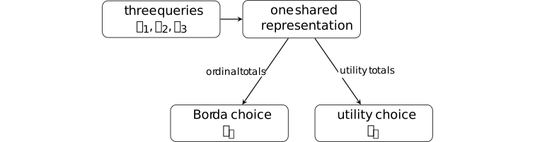
This finite example isolates information lost by ranking. The compromise circuit is never first for an individual query, yet its aggregate utility is largest. It does not show that Borda is always suboptimal or that a neural model must collapse all queries to one representation.
Theorem 2.13. Noiseless preference distortion for deterministic learners [ftip-009A]AGENTDRAFTED
Theorem 2.13. Noiseless preference distortion for deterministic learners [ftip-009A]AGENTDRAFTED
Let \(Q,H\) be nonempty finite sets, let \(\varnothing \neq \mathfrak E\subseteq H^Q\) be finite, and let \(C_0=\{c_1,\ldots ,c_m\}\) be a nonempty finite set of deterministic maps \(Q\to Y\). Write \(N=|Q|\), \(r=|H|\), \(p=|\mathfrak E|\) and \(m=|C_0|\). The query law is uniform on \(Q\). Call \(C_0\) pointwise response-separating when
\[ c_i\neq c_j\quad \Longrightarrow \quad c_i(q)\neq c_j(q) \qquad (q\in Q). \]Assume this separation. Let \(\mathcal A\) be a deterministic preference-only learner: from a pretrained model \(\mathfrak m_0\) and the complete strict ordinal profile, it returns \((e,h,C_0)\) with \(e\in \mathfrak E\) and a possibly stochastic router \(h:H\to \Delta (C_0)\). The comparator class is exactly \(\mathcal M_{\rm det}(C_0)\) of Definition 2.9, including every map \(H\to C_0\) for each \(e\in \mathfrak E\).
For every such pretrained model and learner there exists \(u:Q\times Y\to [0,1]\), inducing a strict profile, such that
\[ \sum _{j=1}^m u(q,c_j(q))=1\quad (q\in Q), \]\[ R_{Q,\mathfrak E,H}=\frac {N}{\sqrt {N(r+\log p)}+r}, \]\[ \operatorname {Dist}_u(\mathcal A;\mathfrak m_0) \geq \frac 1{80}\min \{\sqrt m,R_{Q,\mathfrak E,H}\}. \]Logarithms are natural. Utility averages over the uniform query and the learner's router draw as in Definition 2.6. The comparator maximum exists because its class is finite and nonempty. It is positive for the normalized utilities above: some constant-circuit route has mean at least \(1/m\). A zero learner utility therefore gives distortion \(+\infty \), with no \(0/0\) case.
Proof.
Proof.
First, for every normalized nonnegative utility, the comparator value is at least the learner value. Keep the learner's representation map and, on each fiber, choose a circuit maximizing its total utility there. That deterministic choice dominates the stochastic mixture and belongs to the comparator class. Thus distortion is at least one.
Put
\[ \begin {aligned} D&=\sqrt {Nr}+\sqrt {\frac N2\log (4p)},& B&=\sqrt {N(r+\log p)},\\ T&=\min \{\sqrt m,R_{Q,\mathfrak E,H}\},& x&=\min \{\sqrt m,N/(2D)\}. \end {aligned} \]Since \((\log 4)/2<1\leq r\) and \(\log p\geq 0\), we have \(D\leq 2B\). Consequently \(N/(2D)\geq N/(4B)\geq R_{Q,\mathfrak E,H}/4\) and \(x\geq T/4\). Every denominator is positive.
If \(m=1\), assign utility one to the sole circuit response at every query. Distortion is one and \(T\leq 1\). If \(m\geq 2\) but \(x<2\), assign the same strict normalized values \(2(m-j)/(m(m-1))\) to the circuits in index order at every query. Distortion is at least one and \(T<8\), which proves the claimed bound. Extend both assignments by zero to all other responses.
In the remaining case set \(k=\lfloor x\rfloor \). Then
\[ 2\leq k\leq \sqrt m,\qquad kD\leq N/2, \qquad k\geq x/2\geq T/8. \]Write \([k]=\{1,\ldots ,k\}\) and fix a map \(f:Q\to [k]\) supplied by Lemma 2.15. At a query with label \(i=f(q)\), fix the strict order putting \(c_i\) first and the remaining circuits in increasing index order. Let \(\operatorname {rank}_i(j)\in \{1,\ldots ,m\}\) be the position of \(c_j\), with the first circuit at rank one, and define
\[v_i(j)=\frac {2(m-\operatorname {rank}_i(j))}{m(m-1)}.\]These values decrease strictly in the fixed order, sum to one and lie in \([0,2/m]\). The ordinal profile is now fixed independently of the learner's output. Run the deterministic learner on this profile and \(\mathfrak m_0\), obtaining \((e,h,C_0)\). Write \(h_z(j)=h(z)(c_j)\) for the probability of circuit \(c_j\) at representation \(z\). For each \(z\in H\), choose \(i_z\in [k]\) minimizing \(h_z(j)\) over \(j\in [k]\), breaking ties by index. Since \(\sum _{j=1}^k h_z(j)\leq 1\), we have \(h_z(i_z)\leq1/k\).
Let \(A=\{q:f(q)=i_{e(q)}\}\) and \(S=|A|\). The lower partition bound gives
\[ S=\sum _zX_{z,i_z}\geq \sum _z\min _{j\in [k]}X_{z,j} \geq N/k-D\geq N/(2k). \]Fix \(\epsilon =1/4\). For \(i=f(q)\), assign
\[ u(q,c_j(q))= \begin {cases} (1-\epsilon )\mathbf 1_{j=i}+\epsilon v_i(j),&q\in A,\\ (1-\epsilon )/m+\epsilon v_i(j),&q\notin A. \end {cases} \]Each row is nonnegative and sums to one. On selected queries the added peak favors the already highest-ranked circuit; on the other queries the same constant is added to every circuit. Hence every row induces exactly the fixed strict order. Pointwise response separation makes these assignments well-defined on \(Q\times Y\); assign zero to responses outside the attained circuit responses. Because the final utility has the unchanged ordinal profile, the deterministic learner returns the same \((e,h,C_0)\).
Write \(W=NU\) for total utility. A selected query gives the learner at most \((1-\epsilon )/k+2\epsilon/m\); any other query gives at most \((1-\epsilon )/m+2\epsilon/m\). Averaging over the stochastic router yields
\[ W_{\mathcal A} \leq (1-\epsilon )S/k+(1-\epsilon )(N-S)/m+2\epsilon N/m \leq S/k+2N/m. \]Choose the deterministic comparator \(e^*=e\) and \(h^*(z)=c_{i_z}\). It belongs to the declared class, attains utility at least \(1-\epsilon \geq1/2\) on each selected query and nonnegative utility elsewhere. Thus its total utility is at least \(S/2\). If learner utility is zero the bound follows. Otherwise, using \(S\geq N/(2k)\) and \(k^2\leq m\),
\[ \begin {aligned} \operatorname {Dist}_u &\geq \frac {S/2}{S/k+2N/m} =\frac {k}{2(1+2kN/(mS))}\\ &\geq \frac {k}{2(1+4k^2/m)} \geq \frac {k}{10}\geq \frac {T}{80}. \end {aligned} \]Appendix Theorem A.1 of The limits of preference data for post-training[zhao2025limits] states the corresponding rate for its routing model. Its displayed balancing parameter retains \(\log N\) factors that are absent from its final rate; the second-moment partition bound in Lemma 2.15 supplies a separate argument for the stated restricted model. Its index-based perturbation on queries outside the selected group need not preserve their prescribed favorite; the query-dependent rank weights used here preserve it. When circuits collide at a query, a circuitwise prescription need not define a response utility; pointwise separation excludes that issue.
The utility is a worst-case existential choice for each fixed learner. The proof permits stochastic inference, but it does not cover internal learner randomness: a utility chosen after a realized random output need not be one utility valid before the learner's random draw. No claim about response-colliding circuits or the separate noisy-preference bound follows.
Corollary 2.14. A square-root corollary under explicit query growth [ftip-009B]AGENTDRAFTED
Corollary 2.14. A square-root corollary under explicit query growth [ftip-009B]AGENTDRAFTED
Under all hypotheses of Theorem 2.13, including a deterministic preference-only learner and pointwise response separation, assume
\[R_{Q,\mathfrak E,H}\geq \sqrt {|C_0|}.\]For every pretrained model and every such learner, the utility supplied by that theorem satisfies
\[ \operatorname {Dist}_u(\mathcal A;\mathfrak m_0) \geq \frac 1{80}\sqrt {|C_0|}. \]
Proof.
Proof.
The displayed growth condition makes the minimum in Theorem 2.13 equal to \(\sqrt {|C_0|}\).
Theorem 3.3 of The limits of preference data for post-training[zhao2025limits] gives a square-root rate in its large-query regime. The explicit condition above gives a finite regime for the reconstructed theorem with its stated learner and response assumptions.
Lemma 2.15. A simultaneous finite partition bound [ftip-009C]AGENTDRAFTED
Lemma 2.15. A simultaneous finite partition bound [ftip-009C]AGENTDRAFTED
Let \(Q,H\) be nonempty finite sets with \(N=|Q|\) and \(r=|H|\), and let \(\mathfrak E\subseteq H^Q\) be nonempty and finite with \(p=|\mathfrak E|\). For every integer \(k\geq 1\), there is a map \(f:Q\to [k]\) such that, simultaneously for every \(e\in \mathfrak E\),
\[ \begin {aligned} \sum _{z\in H}\max _{j\in [k]}X_{z,j}&\leq \frac Nk+D,\\ \sum _{z\in H}\min _{j\in [k]}X_{z,j}&\geq \frac Nk-D, \end {aligned} \]where \([k]=\{1,\ldots ,k\}\), logarithms are natural, and
\[ X_{z,j}=|\{q\in Q:e(q)=z,\ f(q)=j\}|, \qquad D=\sqrt {Nr}+\sqrt {\frac N2\log (4p)}. \]
Proof.
Proof.
Choose the labels \(f(q)\) independently and uniformly from \([k]\). Fix \(e,z\), write \(n_z=|e^{-1}(z)|\), and put \(a_j=X_{z,j}-n_z/k\). Each occupancy has variance \(n_z(1/k)(1-1/k)\), so
\[\mathbb E\sum _{j=1}^k a_j^2=n_z(1-1/k).\]The pointwise maximum and minimum satisfy
\[ \begin {aligned} \max _jX_{z,j}&\leq n_z/k+\|a\|_2,\\ \min _jX_{z,j}&\geq n_z/k-\|a\|_2. \end {aligned} \]Jensen's inequality gives \(\mathbb E\|a\|_2\leq \sqrt {n_z(1-1/k)}\). Summing over \(z\) and applying Cauchy--Schwarz yields
\[ \begin {aligned} \mathbb E\sum _z\max _jX_{z,j}&\leq N/k+\sqrt {Nr(1-1/k)},\\ \mathbb E\sum _z\min _jX_{z,j}&\geq N/k-\sqrt {Nr(1-1/k)}. \end {aligned} \]Changing one label changes only one representation group: one occupancy decreases by one and another increases by one. Its maximum and its minimum each change by at most one. Thus both sums have bounded differences with all \(N\) constants equal to one. McDiarmid's inequality, also used in Appendix A.1 of The limits of preference data for post-training[zhao2025limits], bounds each relevant one-sided deviation of size \(t\) by \(\exp (-2t^2/N)\).
Choose \(t=\sqrt {(N/2)\log (4p)}\). A union bound over both tails and all \(p\) representations gives total failure probability at most
\[2p\exp (-2t^2/N)=\frac 12<1.\]At least one deterministic labeling satisfies both claimed bounds, since \(\sqrt {Nr(1-1/k)}\leq \sqrt {Nr}\). Empty representation fibers have all occupancies zero and require no exception.
The bound uses a second-moment estimate in place of the occupancy estimate in source Lemma A.2. The chosen labeling depends only on \(Q,H,\mathfrak E,k\); its existence uses proof randomness and does not assume randomness in the learning algorithm.
Definition 2.16. Bradley--Terry preference from a score map [ftip-009D]AGENTDRAFTED
Definition 2.16. Bradley--Terry preference from a score map [ftip-009D]AGENTDRAFTED
Fix a query \(\xi \) and nonnegative circuit scores \(a_{\xi ,c}\geq 0\) such that \(a_{\xi ,c_i}+a_{\xi ,c_j}>0\) for every compared pair. The Bradley--Terry comparison law is
\[ \Pr (c_i\succ _{\xi }c_j) =\frac {a_{\xi ,c_i}} {a_{\xi ,c_i}+a_{\xi ,c_j}}. \]Only score ratios are identified: multiplying every score for a fixed query by the same positive constant leaves all comparison probabilities unchanged. The linear and exponential score links discussed in [zhao2025limits, Section 3.2] therefore impose different assumptions on the relation between rewards and comparisons.
Definition 2.17. Exponential-score Bradley--Terry feedback [ftip-009E]AGENTDRAFTED
Definition 2.17. Exponential-score Bradley--Terry feedback [ftip-009E]AGENTDRAFTED
The exponential-score link sets
\[ a_{\xi ,c}=\exp \left (u(\xi ,c(\xi ))\right ). \]For this link, exact comparison probabilities reveal pairwise utility differences through
\[ \log \frac {\Pr (c_i\succ _{\xi }c_j)} {\Pr (c_j\succ _{\xi }c_i)} =u(\xi ,c_i(\xi ))-u(\xi ,c_j(\xi )). \]This algebra explains why a known link and infinite noiseless frequency information can expose more than an ordinal order. It does not apply when the link is unknown or misspecified.
Definition 2.18. Linear-score Bradley--Terry feedback [ftip-009F]AGENTDRAFTED
Definition 2.18. Linear-score Bradley--Terry feedback [ftip-009F]AGENTDRAFTED
The linear-score link sets
\[ a_{\xi ,c}=u(\xi ,c(\xi )), \qquad \Pr (c_i\succ _{\xi }c_j) =\frac {u(\xi ,c_i(\xi ))} {u(\xi ,c_i(\xi ))+u(\xi ,c_j(\xi ))}. \]Write \(p^u_{\xi ,ij}\) for the displayed probability and define the complete pairwise-probability profile
\[ P_u^{\rm lin} =\left (p^u_{\xi ,ij}\right )_{\xi \in Q,\,c_i\neq c_j\in C_0}. \]This requires nonnegative utilities and a positive denominator for each queried pair. A linear-score algorithm \(\mathcal A_{\rm lin}\) takes \((\mathfrak m_0,P_u^{\rm lin})\) as input and returns \(\mathfrak m_{\mathcal A_{\rm lin}}(u)\). The following lower bound concerns this specific link; it is not a lower bound for every stochastic preference model.
Theorem 2.19. General linear-score noisy preference lower bound [ftip-009G]AGENTDRAFTED
Theorem 2.19. General linear-score noisy preference lower bound [ftip-009G]AGENTDRAFTED
Assume pointwise response separation as defined in Theorem 2.13. For every pretrained routing model and linear-score algorithm \(\mathcal A_{\rm lin}\), there exists a utility
\[ u:Q\times Y\longrightarrow [0,1]. \]Post-training from even the complete comparison-probability profile of the linear-score link then satisfies
\[ \operatorname {Dist}_u(\mathcal A_{\rm lin};\mathfrak m_0) \geq \widetilde \Omega \left ( \min \left \{|C_0|,R_{Q,\mathfrak E,H}\right \} \right ), \]where \(R_{Q,\mathfrak E,H}\) is defined in Theorem 2.13. The theorem is again existential in \(u\) and uses the source's deterministic comparator. The same circuitwise-utility issue recorded in Theorem 2.13 prevents us from asserting the source's unrestricted pretrained-model quantifier here. Its noise is informative because probabilities depend on cardinal scores; the obstruction survives under the particular linear link.
This lower bound is the form of Appendix Theorem A.5 in The limits of preference data for post-training[zhao2025limits] with the additional pointwise response-separation assumption stated above.
Remark 2.20. The noisy main theorem and appendix have different asymptotic notation [ftip-009H]AGENTDRAFTED
Remark 2.20. The noisy main theorem and appendix have different asymptotic notation [ftip-009H]AGENTDRAFTED
The main-text Theorem 3.4 of The limits of preference data for post-training[zhao2025limits] displays \(\Omega (|C_0|)\) in its stated large-query regime. Appendix Theorem A.5 displays the general bound with \(\widetilde \Omega \) and the minimum in Theorem 2.19. The tilde can hide logarithmic factors, so these statements are not textually identical.
The general bound in Theorem 2.19 has the appendix's rate with a possible logarithmic loss. Eliminating that loss to obtain the main-text rate requires an additional argument.
Definition 2.21. Cardinal value query [ftip-009I]AGENTDRAFTED
Definition 2.21. Cardinal value query [ftip-009I]AGENTDRAFTED
In the social-choice source, agents rank alternatives and also have nonnegative cardinal values. A value query takes an agent \(i\) and an alternative \(j\) and returns \(v_{ij}\) [amanatidis2021peeking, Definition 1].
Under the routing analogy, a query \(\xi \in Q\) plays the role of an agent and a circuit \(c\in C_0\) plays the role of an alternative. A cardinal query therefore reveals one value \(u(\xi ,c(\xi ))\). Query counts inherited from the social-choice theorem are per query/agent, not totals across \(Q\).
Theorem 2.22. Acceptable Range Voting information--distortion tradeoff [ftip-009J]AGENTDRAFTED
Theorem 2.22. Acceptable Range Voting information--distortion tradeoff [ftip-009J]AGENTDRAFTED
Let \(m\) be the number of alternatives and let \(k\in \{1,\ldots ,m\}\). Theorem 4 of Peeking behind the ordinal curtain: Improving distortion via cardinal queries[amanatidis2021peeking] states that \(k\)-Acceptable Range Voting uses
\[ O(k\log m) \]value queries per agent and has distortion
\[ O\left (m^{1/(k+1)}\right ). \]This is a social-choice mechanism theorem. It transfers directly to the singleton-representation specialization \(|H|=1\), where every query must use one common circuit. Under that restriction, queries are agents and circuits are alternatives as in Definition 2.21. The theorem does not by itself cover a routing comparator that may choose different circuits for different representations, and it is not an implementation of neural post-training.
This statement is Theorem 4 of Peeking behind the ordinal curtain: Improving distortion via cardinal queries[amanatidis2021peeking].
Corollary 2.23. Constant distortion with logarithmically many value queries per query [ftip-009K]AGENTDRAFTED
Corollary 2.23. Constant distortion with logarithmically many value queries per query [ftip-009K]AGENTDRAFTED
Taking \(k\) proportional to \(\log m\) in Theorem 2.22 yields constant distortion with
\[ O(\log ^2 m) \]value queries per agent. This is Corollary 2 of Peeking behind the ordinal curtain: Improving distortion via cardinal queries[amanatidis2021peeking], inherited as Theorem 3.5 by The limits of preference data for post-training[zhao2025limits]. Under the routing analogy, the count is per query, so a full table over \(|Q|\) queries can require \(O(|Q|\log ^2m)\) values. The statement is an upper bound for the named mechanism in the common-circuit specialization of Theorem 2.22. It is not a result for the full routing comparator, nor a lower bound saying that this many values are necessary.
Remark 2.24. Information and optimization assumptions in the two finite models [ftip-009L]AGENTDRAFTED
Remark 2.24. Information and optimization assumptions in the two finite models [ftip-009L]AGENTDRAFTED
The two source families assume different information models; the diagram compares them without imposing an information order.
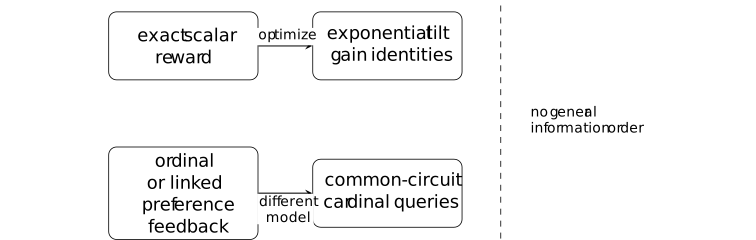
The KL identities characterize the exact optimizer for a declared scalar reward. The preference lower bounds are worst-case statements inside a fixed- circuit routing model. Bradley--Terry conclusions depend on the chosen score link. In the common-circuit specialization, cardinal queries change the information modality and admit a positive mechanism result. Outside that specialization, the preference and cardinal-query results are not directly comparable without further assumptions.
None of these statements derives the finite transcript theorem Theorem [ftip-007S], and none proves that benchmark gain is capability acquisition. Applying either result to a training system requires that system to satisfy the corresponding information, optimizer, and comparator assumptions.