A capability claim in this note names four objects:

1. a starting model artifact \(M_0\), with its accompanying information, libraries, tools and initially available controllers disclosed;
2. a procedure \(A\) that may query models, interact, retain experience and train successor artifacts, with its feedback sources specified;
3. an evaluation rule \(E\), including the task law, retained artifact and deployment procedure being evaluated; and
4. a resource bound \(b\).

The claim concerns the observable outcome of running \(A\) from \(M_0\) and judging the result with \(E\) while respecting \(b\). It is not a claim about an unbounded or unspecified model.

For a comparison across generations, use the complete lineage specification to make these initial resources and permitted operations explicit. Newly generated controllers and learned artifacts belong to the charged process. An externally supplied contribution has a declared producer and acquisition procedure; it is not silently added to the starting model's resources.

The bound \(b\) may contain several coordinates, such as training tokens, rollouts, accelerator work, wall-clock time, tool calls, or evaluation-time samples. Distinguish the complete development budget from the deployment budget used to compare frozen artifacts on fresh problems. Coordinates with different units remain separate unless a declared cost model converts them to a common unit.

This convention follows the experimental separation between training and inference procedures used in [shao2024deepseekmath, secs. 3--4] and [guo2025deepseek, secs. 2--3]. Those studies motivate the objects in a claim; they do not imply that every capability is summarized by one benchmark or one scalar budget.

Holding the model fixed, the comparison isolates how inference procedure and budget alter measured success.

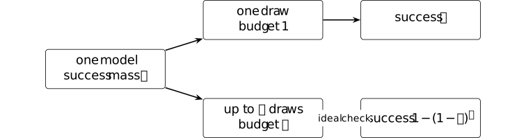
Assume independent draws and a declared perfect checker that recognizes a correct candidate when one appears. The one-draw procedure succeeds with \(J_1=p\). A procedure allowed up to \(k\) draws succeeds whenever not all draws fail: \[ J_k=1-(1-p)^k. \] Both procedures query the same conditional distribution.

Policy performance under a specified interaction and evaluation procedure is standard in [sutton2018reinforcement, Section 3.5]. The formula demonstrates procedural dependence. Independence and a perfect checker are declared toy assumptions, not properties attributed to a frontier language model.

Fix a capability claim in Convention 1.1, a prespecified successful behaviour event \(B\), and a tolerance \(\varepsilon >0\). Let \(p_0(B)\) be the probability of \(B\) under the declared starting procedure and \(p_1(B)\) its probability after the intervention, both measured by the same evaluator. An elicitation witness is an observed increase \[ p_1(B)>p_0(B)\quad \text {with}\quad p_0(B)\geq \varepsilon . \] It witnesses improved access to behaviour that was already observable at the declared starting budget.

The event \(B\), tolerance \(\varepsilon \), sampling procedure, and confidence rule are part of the claim. Changing any of them changes what the witness means.

Reinforcement learning can move probability toward successful traces that a base model already emits; this possibility is tested empirically in [liu2025understanding, secs. 2.3 and 3.3--3.4]. A finite experiment cannot establish that an unrestricted generative model assigns exactly zero probability to a behaviour. The positive threshold \(\varepsilon \) therefore belongs to the declared experiment rather than to an ontological claim about what the model ``contains.''

An elicitation witness depends on the sampling budget, decoding rule, and reward. Bounding the attainable increase in \(p_1(B)\) requires assumptions about the starting probability \(p_0(B)\) and the information supplied by post-training.

Fix a capability claim in Convention 1.1, a prespecified transfer evaluation \(E^{+}\), and thresholds \(0\leq \varepsilon _0<\varepsilon _1\leq 1\). Let \(u_0\) and \(u_1\) be the probabilities of passing \(E^{+}\) before and after the intervention, using the same evaluation protocol and budget. An acquisition witness is the pair of inequalities \[ u_0\leq \varepsilon _0 \qquad \text {and}\qquad u_1\geq \varepsilon _1. \] The transfer evaluation must not be used to select training examples, rewards, or checkpoints.

An acquisition witness is operational. It records a large, independently measured change under one declared procedure; it does not prove that the starting model assigned mathematical probability zero to every successful continuation.

Training success alone does not distinguish learning from memorization, selection, or evaluator exploitation. The base-versus-reinforcement-learning comparisons in [yue2025does, secs. 3--5] motivate this distinction, but their empirical criteria are not a universal definition of acquisition.

The thresholds in Definition 1.5 require enough evaluation samples to certify both inequalities. Whether the witness survives a distribution shift depends on the task law; evaluator leakage invalidates its interpretation as independent evidence.

For a finite set \(X\), write \(|X|\) for its cardinality and \(X^*\) for the set of finite sequences with entries in \(X\). A map \(f:X\to Y\) sends \(x\in X\) to \(f(x)\in Y\); the inverse image of \(A\subseteq Y\) is \(f^{-1}(A)=\{x\in X:f(x)\in A\}\).

Write \[ \Delta (X)=\left \{p:X\to [0,1]:\sum _{x\in X}p(x)=1\right \} \] for the probability simplex on \(X\). If \(p\in \Delta (X)\) and \(Z:X\to \mathbb R\), then \[ \mathbb E_{x\sim p}[Z(x)]=\sum _{x\in X}p(x)Z(x). \] A random variable is a map from the sample set to its value set. Random variables \(Z\) and \(W\) are independent under \(p\) when \(p(Z=z,W=w)=p(Z=z)p(W=w)\) for every pair of values \(z,w\).

For nonfinite interaction spaces, probability laws and conditional kernels require the measurable structure described in Remark 2.3.

Using the notation of Notation 2.1, a finite probability law on \(X\) is an element \(p\in \Delta (X)\). For an event \(A\subseteq X\), its probability is \[ p(A)=\sum _{x\in A}p(x). \] For \(p(A)>0\), the conditional law on \(B\subseteq X\) is \(p(B\mid A)=p(A\cap B)/p(A)\).

A finite vocabulary and a bounded token sequence admit probability laws expressed as ordinary sums, with explicit normalization and conditioning. The finite-sequence interface matches [phuong2022formal, sec. 3, Sequence modelling].

States, observations, and tool outputs need not be finite. In that setting \(\Delta (X)\) is replaced by probability measures on a declared measurable space and conditional laws are probability kernels. Results on finite spaces need additional measurable-space hypotheses before they apply in this setting.

A finite vocabulary is a nonempty finite set \(\mathcal V\) of token identifiers. A token identifier is an atomic symbol for the sequence model; it need not be a word or a character.

When termination is represented in-band, choose a distinguished token \(\mathtt {eos}\in \mathcal V\). Other control tokens, if present, are named as elements of the same vocabulary rather than assumed implicitly.

Let \(\Sigma \) be a finite character or byte alphabet and let \(\mathcal V\) be the vocabulary of Definition 2.4. A tokenizer is a specified map \(\tau :\Sigma ^*\to \mathcal V^*\). A detokenizer is a specified map \(\delta :\mathcal V^*\to \Sigma ^*\).

A tokenizer package also fixes its text normalization rule \(N\). When the package promises normalized round trips, the relevant condition is \(\delta (\tau (s))=N(s)\) for text \(s\in \Sigma ^*\); it is not the claim that \(\tau \) and \(\delta \) are inverse bijections on all sequences. SentencePiece keeps the segmentation model and detokenization convention together, which is why both maps belong to the model interface.

Byte-pair encoding gives another construction of \(\tau \). Learned merge operations turn an initial symbol sequence into subword units; see [sennrich2016neural, §3.2]. The learned merges and base alphabet are therefore part of the tokenizer specification.

A four-stage toy tokenizer separates token-level round-trip stability from recovery of the original string.

Here underscores display spaces. Declare \(N(A\_\_B)=a\_b\), \(T(a\_b)=(a,b)\), and \(D(a,b)=a\_b\). For \(s=A\_\_B\), \[ D(T(N(s)))=a\_b\neq s, \qquad T(N(D(T(N(s)))))=(a,b). \] The token sequence is stable after normalization although the original case and repeated space are not recovered.

The source-grounded tokenizer interface is Definition 2.5. The displayed normalization rule belongs only to this finite construction; no such lossy transformation is attributed to SentencePiece.

Let \(\mathcal V\) be the vocabulary of Definition 2.4. A token sequence of length \(n\geq 0\) is written \(x_{1:n}=(x_1,\ldots ,x_n)\in \mathcal V^n\); positions are one-based. Its length is \(|x_{1:n}|=n\), its prefix before position \(t\) is \(x_{<t}=x_{1:t-1}\), and \(x_{<1}\) is the empty sequence. Juxtaposition \(xy\) denotes concatenation.

If \(\mathtt {eos}\) is distinguished, a completed generated continuation \(y_{1:m}\) ends with \(y_m=\mathtt {eos}\) and contains no earlier \(\mathtt {eos}\). A fixed length limit can also stop generation; the stopping mechanism must state which convention it uses.

Let \(\Theta \) be a parameter set. With the probability notation of Notation 2.1 and the sequence convention of Convention 2.7, a conditional next-token law is a family of maps \[ \pi _\theta :\mathcal V^*\longrightarrow \Delta (\mathcal V), \qquad \theta \in \Theta . \] For a prefix \(x_{<t}\) and token \(a\in \mathcal V\), the number \(\pi _\theta (a\mid x_{<t})\) is the probability assigned to choosing \(a\) at position \(t\).

This is the observable probabilistic interface. It does not yet specify the neural computation that produces the distribution.

Fix the next-token law of Definition 2.8, a prompt \(x\in \mathcal V^*\), and a continuation \(y_{1:m}\in \mathcal V^m\). Its autoregressive continuation probability is \[ P_\theta (y_{1:m}\mid x) =\prod _{t=1}^{m} \pi _\theta \left (y_t\mid x y_{<t}\right ). \] Each factor conditions only on the prompt and earlier continuation tokens.

If generation stops on \(\mathtt {eos}\), the law of a completed continuation is restricted to the sequences specified in Convention 2.7. If generation instead stops at a length limit, the terminal event and its probability must be recorded separately.

Along one branch of a three-symbol prefix tree, conditional token laws determine both continuation probability and negative log-likelihood.

Let the vocabulary be \(\{a,b,\mathtt {EOS}\}\) and let \(p_i\) be the displayed conditional probability at step \(i\). The continuation \((b,a,\mathtt {EOS})\) has \[ \Pr (b,a,\mathtt {EOS}\mid a) =p_1p_2p_3, \qquad -\log \Pr =-\sum _{i=1}^{3}\log p_i. \]

The multiplication follows the causal product in [phuong2022formal, Section 3]. Its scope is one fixed finite continuation, leaving both the decoding algorithm and the law over all variable-length outputs unspecified.

Let \(\mathcal D_{\rm doc}\) be a measurable document space and \(\mathcal S\) a finite set of data sources. Source \(s\in \mathcal S\) has a document law \(Q_s\) on \(\mathcal D_{\rm doc}\), and mixture weights \(\alpha \in \Delta (\mathcal S)\) use the simplex notation of Notation 2.1. Let \(T\) be the context length. A token window is \(x_{1:T}\in \mathcal V^T\); a prediction mask is \(m_{1:T}\in \{0,1\}^T\), where \(m_t=1\) means that the token at position \(t\) contributes to the loss.

Let \(\Theta \) be the parameter set used by the next-token law in Definition 2.8. The model parameters at optimizer update \(k\in \{0,1,\ldots ,K\}\) are \(\theta _k\in \Theta \); \(\theta _0\) is the initialization and \(\theta _K\) the stopped parameter value. A minibatch at update \(k\) is \(\mathcal B_k\). Random document draws, window offsets, masks, batch order, and optimizer noise are part of the training run even when the notation suppresses them.

Using Notation 3.1, a pretraining source mixture is the pair \(((Q_s)_{s\in \mathcal S},\alpha )\). It induces the document law \[ Q_{\alpha }(A)=\sum _{s\in \mathcal S}\alpha _s Q_s(A) \] for every document event \(A\): first sample a source \(s\) with probability \(\alpha _s\), then sample a document from \(Q_s\).

The mixture weights specify sampling frequency. They need not equal the fraction of bytes stored in each source. Resampling, epoch boundaries, or temperature-based weights must therefore be recorded as part of \(\alpha \) or its schedule.

Let \(\dagger \) denote rejection. A document filter is a declared map \[ F:\mathcal D_{\rm doc}\longrightarrow \mathcal D_{\rm doc}\cup \{\dagger \}. \] It may retain a document, return a transformed document, or reject it. The lift \(F_{\#}\) applies \(F\) to a finite corpus and removes every \(\dagger \).

A filter specification includes the features it reads, thresholds, transformation rules, and implementation revision. An acceptance rate alone does not determine the retained document law.

Let \(\mathcal M_{\rm doc}\) be the set of finite multisets of documents. A deduplication operator is a map \[ D:\mathcal M_{\rm doc}\longrightarrow \mathcal M_{\rm doc} \] that selects retained representatives according to a declared duplicate relation. The relation may compare complete documents or spans.

The declaration includes normalization, similarity threshold, cluster construction, and representative tie-breaking. Different choices can remove different training events even when they report the same duplicate rate.

For a protected evaluation collection \(\mathcal E\), an evaluation decontamination operator is a map \[ C_{\mathcal E}:\mathcal M_{\rm doc}\longrightarrow \mathcal M_{\rm doc} \] that removes documents or spans matching \(\mathcal E\) under a declared matching rule.

The protected collection, normalization, match granularity, threshold, and removal policy are part of the operator. Decontamination against one released benchmark does not establish independence from every related task.

Let \(\mathcal C_{\mathrm {raw}}\in \mathcal M_{\rm doc}\) be a finite corpus drawn from the source mixture in Definition 3.2. Using the declared document filter, deduplication operator, and evaluation decontamination operator, an ordered pretraining data pipeline returns \[ \mathcal C_{\mathrm {clean}} =C_{\mathcal E}\left (D\left (F_{\#}(\mathcal C_{\mathrm {raw}})\right )\right ). \] Changing the order can change the retained corpus. The pipeline therefore records the order and exact revisions in addition to the three operators.

The source mixture and cleaning pipeline determine different parts of the data law. The mixture in Definition 3.2 describes how raw documents are proposed. The construction in Definition 3.6 determines which proposals survive and how they are transformed. Together with all random seeds and thresholds, they induce a cleaned document law \(Q_{\mathrm {clean}}\).

Kaplan et al. describe the concrete WebText2 dataset in [kaplan2020scaling, sec. 2.3]. Hoffmann et al. report the MassiveText sources and mixture in [hoffmann2022training, Appendix A, Table A1]. A finite released corpus is one realization of such choices, and an undocumented change in them is not identified by a loss--compute curve.

Fix the context length \(T\) from Notation 3.1. A context-window sampler draws cleaned text from the law described in Remark 3.7 and tokenizes it with Definition 2.5. It then chooses a declared offset and returns a length-\(T\) token sequence \(x_{1:T}\) together with metadata that identifies document boundaries.

If fewer than \(T\) tokens remain, the sampler must specify whether it pads, drops the suffix, or joins another document. These choices change both the distribution of contexts and the prediction mask.

A packed training record is a tuple \(\zeta =(x,m,c,M^{\mathrm {doc}})\). It places tokenized segments \(x^{(1)},\ldots ,x^{(r)}\) into the length-\(T\) token array \(x\), records a prediction mask \(m\), and records a segment identifier \(c_t\in \{0,1,\ldots ,r\}\) at each position. The value \(c_t=0\) denotes padding. Its document mask is \[ M^{\mathrm {doc}}_{ts}= \begin {cases} 0,&c_t=c_s\ne 0\text { and }s\leq t,\\ -\infty ,&\text {otherwise}. \end {cases} \] Replacing the causal mask in Definition [ftip-000S] by this mask prevents one packed document from attending to another. We write \(x_t(\zeta )\), \(m_t(\zeta )\), and \(M^{\mathrm {doc}}(\zeta )\) for the corresponding fields.

The prediction mask \(m_t(\zeta )\) from Notation 3.1 is one only at positions whose target token is retained for training. Padding, a segment's first token when no predecessor is present, and any deliberately excluded control token receive mask value zero.

[kaplan2020scaling], Section 2.2, uses fixed-length sequence batches.

[phuong2022formal], Section 7, gives the causal language-model objective.

The proposed data interface additionally specifies the sampler, segment identifiers, document mask, and prediction mask. Those boundary choices are not determined by the high-level training accounts.

These objects describe one admissible data interface. A concrete training run must replace them with its offset, padding, joining, masking, and packing rules.

Let \(\zeta =(x,m,c,M^{\mathrm {doc}})\) be a packed training record from Definition 3.9. Write \(\pi _{\theta ,M^{\mathrm {doc}}(\zeta )}(\,\cdot \mid x_{<t}(\zeta ))\) for the next-token law of Definition 2.8 when every decoder attention layer uses the declared document mask. For a predicted position \(t\geq 2\), its masked token negative log-likelihood is \[ \ell _t(\theta ;\zeta ) =-m_t(\zeta )\log \pi _{\theta ,M^{\mathrm {doc}}(\zeta )} \left (x_t(\zeta )\mid x_{<t}(\zeta )\right ), \] A masked position has zero contribution; an unmasked position penalizes the log probability computed under the same segment boundaries that defined the packed example.

Let \(Q_T\) be the law of packed examples induced by Remark 3.7--Definition 3.9, and assume that its expected number of predicted positions is positive. The population pretraining objective is the expected total token loss divided by the expected number of predicted tokens: \[ L_{\mathrm {pop}}(\theta ) =\frac { \mathbb E_{\zeta \sim Q_T} \left [\sum _{t=2}^{T}\ell _t(\theta ;\zeta )\right ] }{ \mathbb E_{\zeta \sim Q_T} \left [\sum _{t=2}^{T}m_t(\zeta )\right ] }, \] using expectation as fixed in Notation 2.1.

Packing documents into one row requires a block-causal mask so that each token attends only within its own document and to earlier positions there.

For a packed row, set \(M_{ij}=0\) only when tokens \(i,j\) belong to the same document and \(j\leq i\); otherwise set \(M_{ij}=-\infty \). Thus a token in document \(B\) cannot inspect any token in document \(A\), even when \(A\) precedes \(B\) in storage.

The within-document triangle instantiates the causal mask in Definition [ftip-000S]. The block boundary instantiates the packing convention in Definition 3.9. Document-isolated attention is the declared convention in this packed row, not a universal description of pretraining systems.

For a finite training sample of packed records \(\mathcal D_N=(\zeta ^{(i)})_{i=1}^{N}\) with at least one unmasked target token, the empirical pretraining objective is \[ L_N(\theta ) =\frac { \sum _{i=1}^{N}\sum _{t=2}^{T} \ell _t(\theta ;\zeta ^{(i)}) }{ \sum _{i=1}^{N}\sum _{t=2}^{T}m_t(\zeta ^{(i)}) }. \] This is a per-predicted-token average. Reusing or resampling examples changes the stochastic optimization path even when the displayed finite-sample function is unchanged.

The autoregressive token loss follows [phuong2022formal, Section 7]. Kaplan et al. report language-model loss with parameter and compute variables in [kaplan2020scaling, sec. 2.1]. The population ratio-of-expectations in Definition 3.12 and finite per-token ratio in Definition 3.14 are proposed normalization conventions with explicit prediction masks. Neither cited source defines those exact ratios.

A theorem or experiment using another record weighting, length weighting, or expectation order must state that change rather than reuse these symbols.

At update \(k\), let \(\mathcal B_k\) be the minibatch named in Notation 3.1, and let \(N_k=\sum _{\zeta \in \mathcal B_k}\sum _{t=2}^{T}m_t(\zeta )\) be its number of predicted tokens. For \(N_k>0\), the minibatch gradient estimator is \[ g_k=\frac 1{N_k} \sum _{\zeta \in \mathcal B_k}\sum _{t=2}^{T} \nabla _\theta \ell _t(\theta _k;\zeta ), \] where \(\ell _t\) is defined in Definition 3.11. Whether \(g_k\) is unbiased for the gradient of Definition 3.12 depends on the window sampler and minibatch weighting. Other sampling schemes require their own bias statement.

Two equal-length records make a full empirical loss directly comparable with a minibatch estimate, while exposing the assumptions behind unbiasedness.

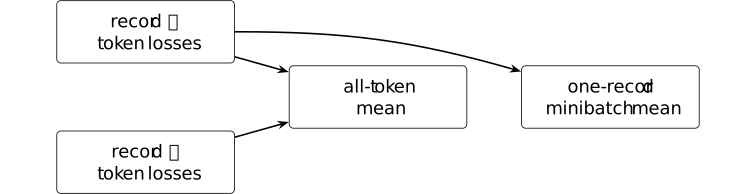
Let \(\ell _{ij}\) denote the token loss at position \(j\) of record \(i\). The full token-average loss is the mean of all \(\ell _{ij}\), while a one-record minibatch averages only the losses from its sampled record. Uniform sampling of equal-length records makes the latter unbiased for the former.

The preceding loss and estimator definitions apply to this equal-length record setup. Equal record lengths make the estimator unbiased here; unequal lengths, padding, dependence, and optimizer noise remain outside its scope.

An optimizer state \(s_k\) is the collection of persistent variables, other than the model parameters \(\theta _k\), that an update rule uses after step \(k\). For Adam, \(s_k\) contains the step index and exponential moving averages of the gradient and squared gradient.

The state is initialized by a declared value \(s_0\). Two runs with the same checkpoint \(\theta _k\) but different optimizer states need not have the same next update.

A parameter update rule is a specified map \(U_k\) that takes the current parameters \(\theta _k\), optimizer state \(s_k\), gradient estimate \(g_k\), and scheduled hyperparameters \(\eta _k\), and returns \[ (\theta _{k+1},s_{k+1}) =U_k(\theta _k,s_k,g_k,\eta _k). \] The learning rate, momentum coefficients, numerical stabilizers, clipping, and weight decay belong to \(\eta _k\) or to the declared form of \(U_k\); they are not determined by the loss alone.

A pretraining run is not determined by minimization of the empirical objective \(L_N\) in Definition 3.14. It includes the initialization, data order, window offsets, dropout and other model randomness, numerical precision, distributed reduction order, optimizer state, every hyperparameter schedule, and a stopping rule. These objects determine a distribution over final parameters even when the source mixture and nominal objective agree.

The training configuration of [vaswani2017attention, sec. 5.3] and the scaling experiments of [kaplan2020scaling, sec. 2.2] report concrete instances of these choices. An optimization result depends on which randomness it averages over and whether the stopping time is fixed or data-dependent.

A base-model artifact is an executable tuple \[ M_0=(\tau ,\delta ,\mathsf {cfg},\theta _K,\mathsf {num}), \] where \(\tau ,\delta \) are the tokenizer and detokenizer of Definition 2.5; \(\mathsf {cfg}\) fixes the architecture of Definition [ftip-0012]; \(\theta _K\) is the stopped pretraining checkpoint; and \(\mathsf {num}\) fixes the numerical and inference conventions required to evaluate its next-token law.

The tokenizer model is part of the executable system by Definition 2.5. A weight file without its vocabulary, architecture configuration, or output convention does not determine the law \(\pi _{\theta _K}\) in Definition 2.8. Training-data and optimizer provenance may accompany the artifact, but they are not runtime inputs.

Section 6 of [phuong2022formal] describes decoder architecture. Sections 3.1 and 3.5 of [kudo2018sentencepiece] treat the tokenizer as a separate model. Public model releases additionally distribute weights, configuration, and numerical conventions. The proposed artifact model in Definition 3.21 includes these runtime ingredients because none alone determines an executable next-token law.

Training provenance accompanies the artifact but is not itself a runtime argument. Later causal claims must distinguish the executable endpoint from the process that produced it.

An executable-artifact manifest separates runtime components from evidence about how the corresponding weights were trained.

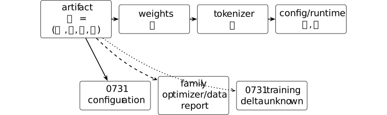
The pinned DeepSeek-V4-Flash-0731 configuration [⧉] declares architecture and numeric-format fields. Sections 2.4 and 4 of the V4 family report [⧉] describe a mixed Muon/AdamW optimizer allocation and pretraining data construction. The exact 0731 data mixture, optimizer schedule, and post-preview training delta remain undisclosed by those sources.

Write \(\mathsf T\) for a task interface, \(\mathcal X_{\mathsf T}\) for its instance set, and \(\mathcal O_{\mathsf T}\) for its candidate-outcome set. A task instance is \(x\in \mathcal X_{\mathsf T}\) and a candidate outcome is \(o\in \mathcal O_{\mathsf T}\). The symbol \(\mu _{\mathsf T}\) denotes a probability law on instances. Equip the instance and outcome sets with declared sigma-algebras; \(\mu _{\mathsf T}\) is a probability measure on the instance sigma-algebra.

Fix an evaluation-resource dimension \(m_{\mathrm {eval}}\geq 1\) and write \(\mathcal B_{\mathrm {eval}}=\mathbb R_+^{m_{\mathrm {eval}}}\) with its coordinatewise order. An evaluation inference protocol is written \(\mathsf I\); its declared evaluation budget is \(b_{\mathrm {eval}}\in \mathcal B_{\mathrm {eval}}\). Its inference-seed set is \(\Omega _I\), with realized seed \(\xi \in \Omega _I\). An evaluator's random-seed set is \(\Omega _E\); its realized seed is \(\omega \in \Omega _E\). It returns utility \(u_{\mathsf T}(x,o;\omega )\in \mathbb R^d\). The dimension \(d\geq 1\) is declared by the evaluation: \(d=1\) gives scalar utility, while \(d>1\) retains several outcomes or costs without an implicit weighting. Equip both seed sets with declared sigma-algebras and \(\mathbb R^d\) with its Borel sigma-algebra. Products below carry the product sigma-algebra; finite or countable discrete spaces may use all subsets. A seed space alone does not specify its sampling law.

A task is a triple \[ \mathsf T=(\mathcal X_{\mathsf T},\mathcal O_{\mathsf T}, \operatorname {Adm}_{\mathsf T}), \] where \(\mathcal X_{\mathsf T}\) is an instance set, \(\mathcal O_{\mathsf T}\) is a candidate-outcome set, and \(\operatorname {Adm}_{\mathsf T}(x,o)\) is a declared well-formedness predicate for an instance-outcome pair.

Admissibility says that an outcome can be interpreted for the instance; it does not say that the outcome is correct, useful, or safe. Those judgments belong to the evaluation utility introduced later.

For the instance set in Definition 4.2, a task law is a probability law \(\mu _{\mathsf T}\) on \(\mathcal X_{\mathsf T}\). An evaluation sample of size \(N\) is a declared joint law of instances \((X_1,\ldots ,X_N)\) whose marginals are \(\mu _{\mathsf T}\); independent sampling is a further assumption, not part of the term ``task law.''

In an episodic control problem this law includes the distribution of starting situations. In a fixed benchmark it may instead be the uniform law on a held-out finite set. Reweighting instances changes the task law even when the instance files are unchanged.

A task and a task law specify admissible instance--outcome pairs and how instances are sampled. Benchmark datasets usually present an input and expect an answer in a parseable format. Reinforcement-learning formulations instead name states, actions, and reward; see [sutton2018reinforcement, Chapter 3]. The admissibility predicate captures parseability, while the law records how instances are sampled. Neither choice already identifies parsing with success.

One-shot inference and an interactive environment can share the same task interface. Claims about an interaction's temporal structure additionally depend on the environment and the observations available at each decision.

Let \(M\) be an executable model artifact of the form in Definition 3.21. An evaluation inference protocol is a specified procedure \[ \mathsf I(M,x,b_{\mathrm {eval}};\xi )=(o,c) \in \mathcal O_{\mathsf T}\times \mathcal B_{\mathrm {eval}}, \] where \(x\in \mathcal X_{\mathsf T}\), \(b_{\mathrm {eval}}\in \mathcal B_{\mathrm {eval}}\), and \(\xi \in \Omega _I\) use the notation of Notation 4.1; \(o\) is a candidate outcome and \(c\in \mathcal B_{\mathrm {eval}}\) is the realized resource-use vector. A valid execution satisfies \(c\preceq b_{\mathrm {eval}}\) coordinatewise.

The protocol fixes prompt construction, decoding, sampling temperature, number of candidates, candidate selection, allowed tools, stopping, and any test-time search. None of these choices is determined by the checkpoint alone.

One next-token law supports many evaluation procedures. Greedy decoding, temperature sampling, majority voting, verifier-guided selection, and multi-round tool use can produce different outcome laws from the same checkpoint. The sampling and selection procedures in [shao2024deepseekmath, secs. 3--4] are concrete examples.

Accordingly, a comparison that changes \(b_{\mathrm {eval}}\) or \(\mathsf I\) does not estimate a training-only effect. A potential frontier therefore depends on evaluation-time compute as well as the trained model.

With the notation of Notation 4.1, an evaluation utility is a declared measurable function \[ u_{\mathsf T}:\mathcal X_{\mathsf T}\times \mathcal O_{\mathsf T}\times \Omega _E\longrightarrow \mathbb R^d, \] where \(\Omega _E\) is the evaluator's measurable seed space. The evaluator applies it only to admissible pairs from Definition 4.2. A deterministic evaluator is the special case in which the value does not depend on \(\omega \in \Omega _E\).

Binary pass-fail evaluation takes \(d=1\) and values in \(\{0,1\}\). A cumulative return is another scalar case. Vector utility keeps qualities such as correctness, safety, latency, and tool cost distinct until a later rule declares how to compare them.

Whenever an expected utility vector is used, its composite evaluation random variable must be measurable and absolutely integrable in every coordinate under the declared joint law. Thus its expectation lies in \(\mathbb R^d\). Bounded measurable utility is a sufficient specialization; so is finite support for the complete evaluation random variable with finite values on that support. Merely taking a finite real value at each seed is insufficient for an unbounded evaluator. The scalar protocol comparison in Convention [ftip-005D] states its joint law explicitly.

Sutton and Barto define scalar episodic return in [sutton2018reinforcement, Section 3.3]. Benchmarks also use exact-match, test, latency, safety, and cost measurements. A proposed seeded vector utility keeps those coordinates separate, with evaluator randomness included in the declared law.

The vector is not a claim that its coordinates share a natural scale. Scalarization, Pareto order, and worst-group summaries are introduced only after the attainable evaluation set is defined.

One fixed policy can receive different measured success rates when the evaluation horizon changes.

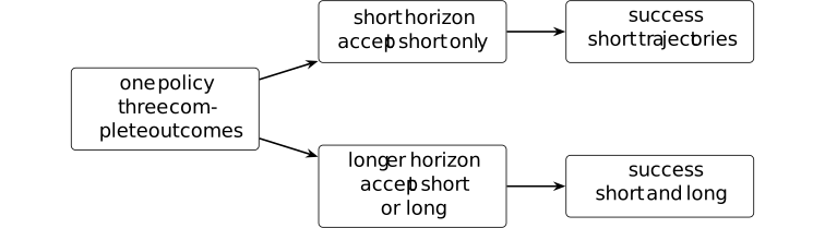
Partition complete trajectories into those that finish within the short horizon, those requiring additional tokens, and failures. The short protocol counts only the first class; the longer protocol may count the first two. Thus the measured score depends on the declared horizon even though the policy is unchanged.

Making an evaluation horizon explicit follows finite-horizon policy evaluation in [sutton2018reinforcement, Chapter 3]. Only truncation is varied here. Larger budgets need not help once decoding rules, tool costs, or selection errors are allowed to change with the budget.

The inference protocol receives only the information designated as public. The public instance \(x\) may include a prompt, tools, and a response schema. Evaluator-only information may include a reference answer, hidden tests, a simulator state, or the evaluator seed \(\omega \). The protocol in Definition 4.5 receives the former and not the latter.

If evaluator-only information influences training, decoding, or candidate selection, the experiment no longer measures performance under the declared information interface. A theorem that assumes an independent evaluator must name the sigma-field or finite data record from which the protocol is excluded.

Let \(\mathcal S,\mathcal O,\mathcal A\) be declared measurable spaces of environment states, public observations, and agent actions. Time is discrete, \(t\in \{0,1,\ldots ,T_{\max }\}\), where \(T_{\max }<\infty \) is a hard horizon. Random states, observations, and actions are \(S_t,O_t,A_t\); lowercase \(s_t,o_t,a_t\) denote realized values. The same convention makes \(h_t\) a realization of \(H_t\) and \(z\) a realization of \(Z\).

The public history available before action \(A_t\) is \(H_t\); the full environment trajectory is \(Z\); and the stopping time is \(\tau _{\mathrm {stop}}\in \{0,1,\ldots ,T_{\max }\}\). Probability kernels are written \(K(dy\mid x)\); on finite spaces this means the probability law \(K(y\mid x)\) and reduces to the notation of Notation 2.1.

With the spaces in Notation 5.1, an initial-state law \(\rho _0(ds_0,do_0)\) is a probability law on \(\mathcal S\times \mathcal O\). It jointly samples the hidden initial state \(S_0\) and the first public observation \(O_0\).

Allowing a joint law covers both a deterministic rendering \(O_0=\operatorname {obs}(S_0)\) and a noisy initial observation. A fixed task instance can be included as a coordinate of \(O_0\); its sampling law is then the task law of Definition 4.3.

A transition-observation kernel at time \(t\) is a probability kernel \[ K_t(ds_{t+1},do_{t+1}\mid s_t,a_t) \] from the current hidden state and action to the next hidden state and public observation. After \(A_t=a_t\), the environment draws \((S_{t+1},O_{t+1})\) from this kernel.

The factorization \(K_t(ds',do'\mid s,a)=P_t(ds'\mid s,a)\,Q_t(do'\mid s',a)\) for declared kernels \(P_t\) and \(Q_t\) recovers the usual separate state-transition and observation kernels when such a factorization is declared. The joint-kernel form does not assume it.

The kernel in Definition 5.3 describes both tools and broader environments. A deterministic tool has a measurable update map \(F_t(s,a)=(s',o')\) and the point-mass kernel concentrated at \(F_t(s,a)\). A stochastic environment permits several next state-observation pairs for the same input.

This distinction matters for replay. Re-executing a deterministic tool call under an unchanged state reproduces its observation, whereas a stored rollout from a stochastic environment is one sample from a conditional law. Any analysis that replaces one with the other needs a coupling or concentration assumption.

At time \(t\), the public history is the alternating sequence \[ H_t=(O_0,A_0,O_1,A_1,\ldots ,A_{t-1},O_t). \] Thus \(H_0=(O_0)\). It contains exactly the observations received and actions taken before the next action \(A_t\); it does not contain the hidden state \(S_t\) unless that state was itself revealed as an observation.

The history in Definition 5.5 contains the agent's available information. The hidden state sequence \((S_0,\ldots ,S_t)\), future observations, evaluator-only tests from Remark 4.10, and future random seeds are absent unless the environment has already exposed them through \(O_0,\ldots ,O_t\).

This boundary determines which policies are implementable. It also separates legitimate memory from leakage: a summary of earlier public observations may be stored in the history, while a hidden reference answer may not be supplied under the same declaration.

A non-anticipating policy is a family of probability kernels \[ \pi _t(da\mid H_t), \qquad t=0,1,\ldots ,T_{\max }-1, \] from public histories in Definition 5.5 to the action space \(\mathcal A\). At time \(t\), the action may depend on \(H_t\) and fresh policy randomness, but not on a later observation or an unobserved state.

A decoder-only language model becomes such a policy only after an inference protocol serializes \(H_t\) into tokens, decodes tokens, and parses them as an action. The next-token law in Definition 2.8 alone does not specify those maps.

A stopping rule is a random time \(\tau _{\mathrm {stop}}\in \{0,1,\ldots ,T_{\max }\}\) such that, for each \(t\), the decision whether \(\tau _{\mathrm {stop}}=t\) is determined by the public history \(H_t\) and any declared stopping randomness available by time \(t\). It cannot inspect future observations.

Stopping can be triggered by a terminal environment observation, an agent action, a resource limit, or the hard horizon. The trigger and the owner of the decision are part of the rule.

If \(\tau _{\mathrm {stop}}=n\), the stopped trajectory is \[ Z=(S_0,O_0,A_0,S_1,O_1,A_1,\ldots , A_{n-1},S_n,O_n). \] It contains the environment states as well as the public action-observation record. Its public projection is the history \(H_n\) of Definition 5.5.

For \(n=0\), the trajectory is \((S_0,O_0)\) and contains no action. A terminal utility may depend on the full trajectory when evaluated inside the environment, even though the policy is restricted to its public projection.

For a task \(\mathsf T=(\mathcal X_{\mathsf T},\mathcal O_{\mathsf T}, \operatorname {Adm}_{\mathsf T})\) from Definition 4.2, an interactive realization is

For each \(x\in \mathcal X_{\mathsf T}\), the law \(\rho _0^x\) is on \(\mathcal S_{\mathsf T}\times \mathcal O^{\rm obs}_{\mathsf T}\), and \(K_t^x\) maps a state and action to the next state-observation law for \(0\leq t<T_{\max }\). The outcome map sends a stopped trajectory \(Z\) to \(\operatorname {out}_{\mathsf T}(x,Z)\in \mathcal O_{\mathsf T}\) and satisfies \(\operatorname {Adm}_{\mathsf T}(x,\operatorname {out}_{\mathsf T}(x,Z))\). For one fixed realization, write its three spaces as the unadorned \(\mathcal S,\mathcal O,\mathcal A\) of Notation 5.1.

The agent policy and stopping rule are not environment fields. They are combined with this realization only when an interaction law is formed.

Section 3.1 of [sutton2018reinforcement] specifies the agent--environment interaction. Section 2 of [kaelbling1998planning] separates hidden state from observation. We combine those ingredients with the task interface of Definition 4.2 so each task instance selects an initial law and transition kernels.

The outcome-extraction map is an additional interface choice; neither cited source supplies it in this task-indexed form. This map connects a stopped interaction to the candidate outcome that the independent evaluator will score.

A deterministic three-action episode records each observation before the next policy decision and ends with an explicit terminal observation.

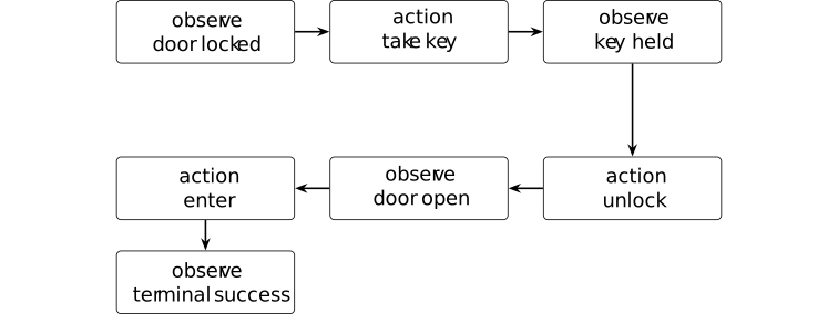
Let \(H_0=(\text {door locked})\). After action \(A_0=\text {take key}\), the environment returns \(O_1=\text {key held}\), so \(H_1=(H_0,A_0,O_1)\). Repeating the same update with unlock and door open, then choosing \(A_2=\text {enter}\), produces \(O_3=\text {terminal success}\) and \(H_3=(H_2,A_2,O_3)\). No later observation is available to an earlier action choice.

The alternating action--observation interface is the finite-history form of the agent setup in [kaelbling1998planning, Section 2]. The trace checks chronology and termination; uncertain state, partial observability, and language-valued actions lie beyond this deterministic instance.

A prefix tree represents token emission as a finite interaction stopped either by an end token or by a hard length cap.

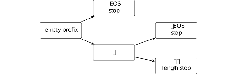
Take vocabulary \(\{a,\mathtt {EOS}\}\). The terminal histories are an immediate end token, an end token after \(a\), and a length-capped history \(aa\). Their probabilities are products of the conditional token laws and sum to one. The last history terminates because the declared maximum length is reached, not because the policy emitted \(\mathtt {EOS}\).

The causal token product is given in [phuong2022formal, Section 3]. The finite representation distinguishes two stopping mechanisms. Token steps remain distinct from tool calls, and unbounded generation is outside the construction.

Sutton and Barto's agent--environment interface in [sutton2018reinforcement, sec. 3.1] supplies alternating states, actions, and rewards. Kaelbling et al. separate hidden state and public observation in [kaelbling1998planning, Section 2]. A stopped interaction is determined by its initial law, transition--observation kernel, policy, and public stopping rule.

The induced interaction law uses four independently declared objects: the initial law \(\rho _0\) in Definition 5.2, the environment kernels \(K_t\) in Definition 5.3, the policy \(\pi _t\) in Definition 5.7, and the stopping rule in Definition 5.8. On finite spaces, the probability of a length-\(n\) trajectory before applying its stopping indicator factors as \[ \rho _0(s_0,o_0) \prod _{t=0}^{n-1} \pi _t(a_t\mid h_t) K_t(s_{t+1},o_{t+1}\mid s_t,a_t). \] The event \(\{\tau _{\mathrm {stop}}=n\}\) selects the stopped trajectories.

This factorization supports later expectations, likelihood ratios, and off-policy reuse. It also exposes an identifiability limit: an outcome distribution by itself generally does not reveal which of the initial law, environment, policy, or stopping rule changed.