Let \(\mathcal X\) be a task-instance set. Write \(\mu _{\rm tr}=\mathcal D_{\rm tr}\) for the training-prompt coordinate of an experiment cell in Definition [ftip-009T]. A training prompt law is this probability law on \(\mathcal X\), used to draw instances during a post-training protocol. Let \(\mu _{\rm ev}\) be an independently declared evaluation law on the same set.

An evaluated prompt slice is a measurable set \(C\subseteq \mathcal X\) with \(\mu _{\rm ev}(C)>0\). Its conditional evaluation law is

The training and evaluation laws need not agree. A slice records where an effect is measured; it does not assert that prompts inside the slice are equally difficult or represented equally in pretraining. We specialize the task-law convention of Definition [ftip-001Q].

A prompt configuration is the record

containing the starting artifact, training prompt law, finite prompt-pool size, reward, update algorithm, and training budget. We call two particular records \(\mathsf c_{\rm nar}\) and \(\mathsf c_{\rm brd}\) only when a cited experiment names them narrow and broad.

Section 4.3 and Appendix F of Demystifying Reinforcement Learning Post-Training of Language Models[clay2026demystifying] instantiate these labels in two model-family experiments. The Qwen comparison uses 100 DeepScaleR prompts versus 10,000 WildChat prompts. The OLMo comparison uses 100 math-only prompts versus 10,000 prompts split evenly among mathematics, instruction following, and code. These labels identify the two reported configurations; they do not define a general measure or ordering of prompt breadth.

The records in Definition 2 change several coordinates together. The prompt-pool size, domain mixture, and repetition frequency differ. Across the paper's Qwen and OLMo studies, the starting artifact and evaluated tasks also differ.

We therefore use ``narrow'' and ``broad'' as names for the source cells. They do not define a total order on prompt laws, and their comparison does not identify a causal effect of breadth alone. A breadth theorem would need a declared statistic and matched configurations that differ only in that statistic.

Fix an evaluated slice \(C\) from Definition 1, and let \(P_0\) and \(P_1\) denote the pre- and post-training protocols whose successful-support probabilities are defined in Definition [ftip-005U]. The slice-conditioned success change is

The evaluation interface, inference budget, and success predicate are held fixed across the two terms. The quantity is an average change on one declared slice. It neither locates the change inside the model nor identifies which training coordinate caused it.

Fix pairwise disjoint evaluated slices \(C_1,\ldots ,C_J\) and a declared degradation threshold \(\kappa >0\). Define the set of materially degraded slices

Degradation is localized relative to this slice family and threshold when \(|\mathcal H_\kappa |=1\). It is distributed when \(|\mathcal H_\kappa |\geq 2\).

These terms depend on the chosen partition, threshold, and evaluation budget. They do not turn a finite benchmark vector into a statement about all capabilities.

Section 5.3 and Appendix F of Demystifying Reinforcement Learning Post-Training of Language Models[clay2026demystifying] supply two OLMo paths; Figure 4 reports their outcomes. Both replace the usual verifiable reward with a random scalar drawn from \(\operatorname {Unif}[0,1]\), but their prompt configurations differ.

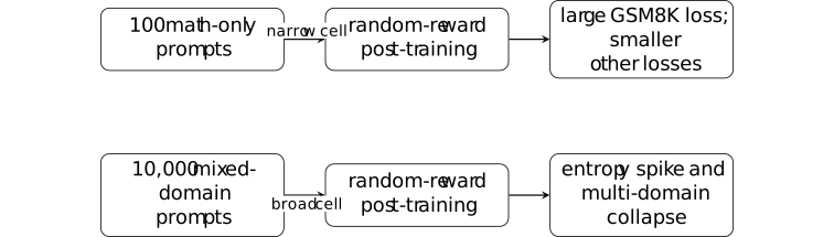
In the narrow SFT-start path, GSM8K accuracy falls from 86 to about 32 by step 400, while the reported MMLU and IFEval changes are much smaller. In the broad path, the source reports an entropy spike near step 400 together with collapse on GSM8K, MMLU, and IFEval. The diagram records that interpretation; it does not isolate prompt breadth from pool size, mixture, or repetition.

Section 5.3 and Figures 3--4 of Demystifying Reinforcement Learning Post-Training of Language Models[clay2026demystifying] report that the Qwen narrow configuration retains higher MATH and AMC Acc@1 than its broad configuration under random reward. The OLMo experiment reports the different evaluation patterns summarized in Example 6.

These are finite empirical observations. The random scalar reward removes task alignment from one feedback channel, but it does not hold all other training coordinates fixed. The reported entropy is a named token statistic, not a direct measure of capability or acquisition.

Let two evaluation slices \(C_1,C_2\) have equal mass. A feedback channel returns an independent Bernoulli reward with mean \(1/2\) under either of two post-training protocols. Suppose their fixed-interface success changes are

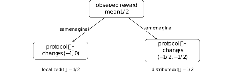
The reward law and its mean are identical, but the slice-level evaluation vectors differ. Hence marginal training reward does not determine whether damage is localized or distributed. This is a finite counterexample, not a claim about the mechanism in the source experiment.

The source cells motivate tests of starting-policy coverage, feedback resolution, and prompt-conditioned damage. They do not establish that dense reward creates mathematical support, that zero sampled hits imply zero probability, or that random reward has one model-independent effect.

Separating the effects of coverage, feedback resolution, and prompt breadth requires stronger controls. One comparison fixes prompt laws and varies only the feedback sigma-algebra. Another fixes feedback and evaluation while varying one starting-policy coordinate. Confidence regions for the complete vector of slice-conditioned changes would quantify effects that an aggregate score can hide.

The reported observations remain conditional on their experimental configurations. They do not establish general results about capability acquisition, elicitation, or the optimal allocation of post-training compute.