Optimizer geometry and representation dependence [ftip-00AU]
✍️source

A scalar objective does not by itself determine a training intervention. This section studies an exact finite-dimensional witness: one represented matrix can have many factor bases, the loss can be constant along that gauge orbit, and an update rule can nevertheless distinguish the bases.

The principal source is the version-one arXiv preprint The loss does not see the basis, but Adam does[singh2026lossbasis]. Its algebraic results assume the stated dimensions, rank conditions, state conventions, and real arithmetic. Experimental observations concern the reported configurations.

1. Factored objectives and gauge symmetry [ftip-00AV]

We first separate a represented matrix from a choice of factors and then separate its full product-preserving symmetry from the orthogonal subgroup that preserves the Euclidean parameter metric.

Notation 1.1. Factored objective and represented matrix [ftip-00AW]

Fix integers $d_1,d_2,k\geq 1$. Let $U\in \mathbb R^{d_1\times k}$ and $V\in \mathbb R^{d_2\times k}$ be factors, let

\[ W(U,V)=UV^{\mathsf T}\in \mathbb R^{d_1\times d_2}, \]

and let $f:\mathbb R^{d_1\times d_2}\to \mathbb R$ be differentiable. The corresponding factored objective is $L(U,V)=f(W(U,V))$. The pair $(U,V)$ is a parameterization; $W(U,V)$ is the represented object on which $f$ depends. This is the rectangular form noted in Section 3 of The loss does not see the basis, but Adam does[singh2026lossbasis].

Definition 1.2. General linear gauge action [ftip-00AX]

For $A\in \mathrm {GL}(k)$, define the general linear gauge action by

\[ \gamma _A(U,V)=(UA,VA^{-\mathsf T}). \]

The inverse transpose on the second factor is essential for a general invertible $A$. When $A=Q\in \mathrm O(k)$, one has $Q^{-\mathsf T}=Q$, and the action becomes $(UQ,VQ)$.

Lemma 1.3. The gauge action preserves the product and loss [ftip-00AY]

For every $A\in \mathrm {GL}(k)$,

\[ W(UA,VA^{-\mathsf T})=UV^{\mathsf T} \quad \hbox {and}\quad L(UA,VA^{-\mathsf T})=L(U,V). \]

Proof.

Since $(VA^{-\mathsf T})^{\mathsf T}=A^{-1}V^{\mathsf T}$, the first identity is $UAA^{-1}V^{\mathsf T}=UV^{\mathsf T}$. Applying $f$ gives the second.

This is the factored-model calculation in Section 3 of The loss does not see the basis, but Adam does[singh2026lossbasis].

Definition 1.4. Orthogonal gauge orbit [ftip-00AZ]

The orthogonal gauge orbit of $(U,V)$ is

\[ \mathcal O(U,V)=\{(UQ,VQ):Q\in \mathrm O(k)\}. \]

Every pair in the orbit represents the same $W$. This orbit is generally smaller than the complete fibre of the map $(U,V)\mapsto UV^{\mathsf T}$. The restriction to $\mathrm O(k)$ is geometric: it preserves the Euclidean metric on factor space.

Lemma 1.5. The orthogonal gauge is the maximal isometric subgroup [ftip-00B0]

The action $\gamma _A$ preserves $\lVert U\rVert _F^2+\lVert V\rVert _F^2$ for every pair $(U,V)$ if and only if $A\in \mathrm O(k)$.

Proof.

If the action is an isometry, take $V=0$ and let one row of $U$ be an arbitrary $u\in \mathbb R^{1\times k}$. Then $\lVert uA\rVert _2=\lVert u\rVert _2$ for every $u$, hence $AA^{\mathsf T}=I$. Conversely, right multiplication by an orthogonal matrix preserves both Frobenius norms.

See Lemma 3.2 and its proof in Appendix B.1 of The loss does not see the basis, but Adam does[singh2026lossbasis].

Lemma 1.6. Gradients transform covariantly along an orthogonal orbit [ftip-00B1]

For $Q\in \mathrm O(k)$,

\[ \nabla _U L(UQ,VQ)=\nabla _U L(U,V)Q, \qquad \nabla _V L(UQ,VQ)=\nabla _V L(U,V)Q. \]

Proof.

Put $G=\nabla f(W)$. Then $\nabla _U L=GV$ and $\nabla _V L=G^{\mathsf T}U$. The represented matrix, and hence $G$, is unchanged along the orbit. Substitution gives both identities.

See Lemma 4.1 and its proof in Appendix B.2 of The loss does not see the basis, but Adam does[singh2026lossbasis].

Definition 1.7. Optimizer state action [ftip-00B2]

Use the optimizer-state convention of Definition [ftip-001H]. For every $Q\in \mathrm O(k)$, an optimizer state action is a map $\sigma _Q:\mathcal S_{\rm opt}\to \mathcal S_{\rm opt}$ compatible with the shapes of the factor states and satisfying $\sigma _Q(s_0)=s_0$ for the declared initial state.

For example, a momentum buffer shaped like $U$ transforms by right multiplication by $Q$; a shared scalar second moment is fixed. An entrywise second-moment array need not admit a state action compatible with every orthogonal $Q$.

Definition 1.8. Gauge-equivariant optimizer [ftip-00B3]

Let $\mathcal A$ be a deterministic instance of the parameter-update rule of Definition [ftip-001I], acting on $(U,V,s)$. It is gauge-equivariant when for every $Q\in \mathrm O(k)$ there is a state action $\sigma _Q$ such that gauge-related initial states produce

\[ (\widetilde U_t,\widetilde V_t,\widetilde s_t) =(U_tQ,V_tQ,\sigma _Q(s_t)) \qquad (t\geq 0). \]

This is Definition 3.1 of The loss does not see the basis, but Adam does[singh2026lossbasis]. Any randomness, schedules, stopping rule, and mixed update blocks must also be coupled as required by Remark [ftip-001J]; the definition does not hide them.

Example 1.9. A commuting optimizer square [ftip-00B4]

One update of a gauge-equivariant optimizer makes the following square commute. The vertical arrows change factor basis and the horizontal arrows apply the same declared update.

$\text{[math]}$

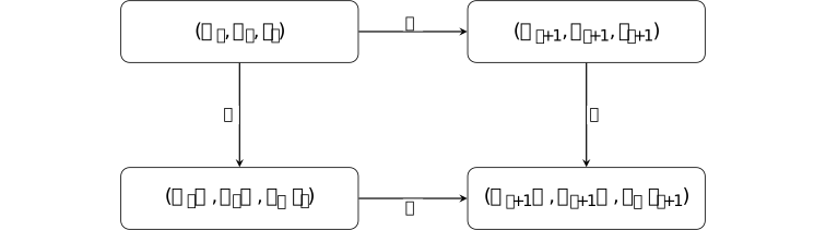
Commutation is stronger than equality of the scalar losses before the step. It states equality of the represented product trajectory after aligning the parameter bases.

Remark 1.10. Product symmetry is larger than the isometric gauge [ftip-00B5]

The full $\mathrm {GL}(k)$ action in Definition 1.2 preserves $W$, but ordinary Euclidean gradients are covariant under the orthogonal specialization used in Lemma 1.6. A theorem for $(UQ,VQ)$ must therefore not be silently promoted to every product-preserving reparameterization.

The source calls the orthogonal subgroup the gauge in its optimizer classification while also noting the larger function-preserving group. These are compatible statements only when their different geometric scopes remain explicit.

2. Equivariant and basis-sensitive update rules [ftip-00B6]

Gradient covariance supplies a test for update rules. Linear and full-matrix operations can commute with a latent rotation, whereas a fixed nonlinear map applied separately to coordinates selects a preferred basis.

Definition 2.1. Memoryless right-equivariant update [ftip-00B7]

A memoryless factor-update map is a function $\Phi :\mathbb R^{n\times k}\to \mathbb R^{n\times k}$ applied to a current gradient $G$ without a persistent optimizer state. It is right-equivariant when

\[ \Phi (GQ)=\Phi (G)Q \qquad (G\in \mathbb R^{n\times k},\ Q\in \mathrm O(k)). \]

This local definition is the input of Theorem 4.5 in The loss does not see the basis, but Adam does[singh2026lossbasis]. It does not classify stateful optimizers such as Adam.

proposition 2.2. Gradient descent and momentum preserve the orthogonal gauge [ftip-00B8]

Gradient descent and Polyak or Nesterov momentum are gauge-equivariant when their factor gradients, momentum buffers, schedules, and look-ahead points are transformed consistently.

Proof.

By Lemma 1.6, $G_t$ becomes $G_tQ$. Gradient descent therefore sends $U_tQ$ to $(U_t-\eta _tG_t)Q$. A momentum buffer initialized at zero and formed by linear combinations of covariant gradients transforms as $M_tQ$; a Nesterov look-ahead point is likewise the reference look-ahead right-multiplied by $Q$. Induction proves the claim.

Proposition 4.2(1) and its proof are in Appendix B.3 of The loss does not see the basis, but Adam does[singh2026lossbasis].

proposition 2.3. A shared scalar second moment preserves the orthogonal gauge [ftip-00B9]

Replace Adam's entrywise second-moment denominator by one scalar whose updates depend only on gauge-invariant quantities such as the pooled mean of the squared entries of both factor gradients. With a covariant first-moment buffer, the resulting stateful update is gauge-equivariant.

Proof.

The first moment is a linear exponential average and transforms by right multiplication by $Q$. The pooled squared-entry mean is the joint squared Frobenius norm divided by the entry count, hence is unchanged by $G\mapsto GQ$. Its bias correction and positive scalar denominator are unchanged, so the complete update transforms covariantly.

Proposition 4.2(2) and its proof are in Appendix B.3 of The loss does not see the basis, but Adam does[singh2026lossbasis]. The result concerns this declared shared-scalar variant, not stock Adam.

proposition 2.4. Full-matrix Muon and Shampoo preserve the orthogonal gauge [ftip-00BA]

Fix one factor, write $n\in \{d_1,d_2\}$ for its row dimension, and let $G_t,M_t\in \mathbb R^{n\times k}$ be its gradient and Muon momentum buffer. For $0\leq \beta <1$, $M_{-1}=0$, and the source's linear momentum update $M_t=\beta M_{t-1}+G_t$, Muon's direction is $\Delta _t=\operatorname {msign}(M_t)$. Under real arithmetic this stateful update and the source's damped Shampoo update are right-equivariant. The Muon claim includes the stated finite Newton--Schulz approximations; the Shampoo claim uses its complete left and right accumulators.

Proof.

By Lemma 1.6, the primed gradient is $G'_t=G_tQ$. Starting from $M'_{-1}=M_{-1}Q=0$, induction through the linear momentum update gives $M'_t=M_tQ$. If $M_t=A\Sigma B^{\mathsf T}$ is a compact singular-value decomposition, then $M_tQ=A\Sigma (Q^{\mathsf T}B)^{\mathsf T}$, so $\operatorname {msign}(M_tQ)=\operatorname {msign}(M_t)Q$. For $\epsilon _{\rm NS}>0$, the Newton--Schulz initialization $X_0=M_t/(\lVert M_t\rVert _F+\epsilon _{\rm NS})$ is covariant because its Frobenius normalization is invariant; each polynomial iterate formed from $X_j$ and $X_jX_j^{\mathsf T}$ preserves the same covariance. For Shampoo, the left accumulator is invariant while the right accumulator transforms by $R_t\mapsto Q^{\mathsf T} R_t Q$. Orthogonal functional calculus conjugates the right matrix function, so the transformed update is the original update right-multiplied by $Q$.

Proposition 4.2(3)--(4) and its proof are in Appendix B.3 of The loss does not see the basis, but Adam does[singh2026lossbasis]. Variable splitting, coordinatewise clipping, mixed update rules, finite precision, and different damping conventions lie outside this statement. The Muon part is stateful; it does not replace the momentum buffer by the current gradient or invoke the memoryless classification of Definition 2.1.

proposition 2.5. Coordinatewise equivariance forces linearity [ftip-00BB]

Let $k\geq 2$ and let a memoryless update have the fixed entrywise form $\Phi (G)_{ij}=\phi (G_{ij})$. If $\Phi (GQ)=\Phi (G)Q$ for every $G$ and $Q\in \mathrm O(k)$, then $\phi (x)=cx$ for some $c\in \mathbb R$.

Proof.

It suffices to use one row and rotations in the first two coordinates. Equivariance at zero gives $\phi (0)=0$. Rotating $(x,0)$ through an angle whose cosine is $a\in [-1,1]$ gives $\phi (ax)=a\phi (x)$. For nonzero $x,y$, compare each with a third number of at least their absolute magnitudes; the ratio $\phi (x)/x$ is constant.

Proposition 4.3 and its proof are in Appendix B.4 of The loss does not see the basis, but Adam does[singh2026lossbasis]. No continuity assumption is needed.

Corollary 2.6. Fixed nonlinear coordinatewise updates break the gauge [ftip-00BC]

A nonlinear fixed entrywise update applied at a zero optimizer state is not gauge-equivariant when $k\geq 2$. In particular, the source applies proposition 2.5 to the first-step maps of Adam, RMSProp, signSGD, and Lion; it checks Adafactor separately because its factored statistics are not an entrywise map.

This is a first-step obstruction. It suffices to disprove equivariance of the full run, but it does not classify every later state or say that such an optimizer cannot reach a particular solution.

Definition 2.7. First-step Adam map and gauge defect [ftip-00BD]

Fix $\epsilon >0$. For zero-state, bias-corrected Adam define the entrywise first-step direction

\[ D_\epsilon (G)=G\mathbin {\oslash }(|G|+\epsilon ) \]

and, for $Q\in \mathrm O(k)$, define its gauge-aligned defect by

\[ E_Q(G)=D_\epsilon (GQ)Q^{\mathsf T}-D_\epsilon (G). \]

Here $|G|$, addition, and division are entrywise. Bias correction makes the first direction independent of Adam's two decay coefficients under the declared convention [singh2026lossbasis, Proposition 4.4].

proposition 2.8. Exact represented-matrix defect after one Adam step [ftip-00BE]

Let $G_U=\nabla _UL(U_0,V_0)$, $G_V=\nabla _VL(U_0,V_0)$, $D_U=D_\epsilon (G_U)$, and $D_V=D_\epsilon (G_V)$. Let $W_1$ be the product after one Adam step from $(U_0,V_0)$ and $\widetilde W_1$ the product after one step from $(U_0Q,V_0Q)$. Then

\[ \begin {aligned} \widetilde W_1-W_1={}&-\eta \bigl (E_Q(G_U)V_0^{\mathsf T} +U_0E_Q(G_V)^{\mathsf T}\bigr )\\ &+\eta ^2\bigl (E_Q(G_U)D_V^{\mathsf T} +D_UE_Q(G_V)^{\mathsf T} +E_Q(G_U)E_Q(G_V)^{\mathsf T}\bigr ). \end {aligned} \]

Proof.

Gauge-align the rotated factors back by $Q^{\mathsf T}$. They are $U_0-\eta (D_U+E_Q(G_U))$ and $V_0-\eta (D_V+E_Q(G_V))$. Multiply, subtract $(U_0-\eta D_U)(V_0-\eta D_V)^{\mathsf T}$, and collect powers of $\eta $.

Proposition 4.4 and its proof are in Appendix B.5 of The loss does not see the basis, but Adam does[singh2026lossbasis].

Example 2.9. A two-coordinate Adam defect witness [ftip-00BF]

Take $d_1=d_2=1$, $k=2$, $f(w)=w^2/2$, $U_0=V_0=(1,0)$, and

\[ Q=2^{-1/2}\begin {pmatrix}1&1\\-1&1\end {pmatrix}. \]

The original and rotated products after one zero-state Adam step are

\[ W_1=\left (1-\frac {\eta }{1+\epsilon }\right )^2, \qquad \widetilde W_1=\left (1-\frac {\eta }{2^{-1/2}+\epsilon }\right )^2. \]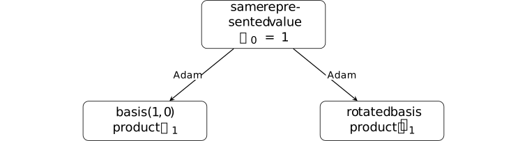 $\text{[math]}$

They differ when $0<\eta <2^{-1/2}+\epsilon $. This is the explicit witness in Proposition 4.4 of The loss does not see the basis, but Adam does[singh2026lossbasis]; it is a statement about one factored quadratic, not about language-model performance.

Example 2.10. A rotated sign update fails to commute [ftip-00BG]

For $G=(1,1)$ and the 45-degree rotation matrix $Q$ of Example 2.9, one has $GQ=(0,\sqrt 2)$. With $\operatorname {sign}(0)=0$,

\[ \operatorname {sign}(GQ)=(0,1), \qquad \operatorname {sign}(G)Q=(0,\sqrt 2). \]

Thus even this two-coordinate update violates the commuting equation in Definition 2.1. The calculation is the explicit Appendix B.4 witness of The loss does not see the basis, but Adam does[singh2026lossbasis].

Theorem 2.11. Full-rank memoryless equivariant rules are Gram-determined [ftip-00BH]

Let $k\leq n$, and let $\Phi $ be defined on full-column-rank matrices $G\in \mathbb R^{n\times k}$. Then $\Phi (GQ)=\Phi (G)Q$ for every $Q\in \mathrm O(k)$ if and only if there is a matrix-valued function $H$ of $GG^{\mathsf T}$ such that

\[ \Phi (G)=H(GG^{\mathsf T})G. \]

Proof.

The displayed form is immediately equivariant. Let $G^+$ denote the Moore--Penrose pseudoinverse. Conversely, set $X(G)=\Phi (G)G^+$. Then $X(G)G=\Phi (G)$ and $X(GQ)=X(G)$. Two full-column-rank matrices with the same left Gram matrix have the same range and differ by a right orthogonal factor. Hence $X(G)$ depends only on $GG^{\mathsf T}$; take $H=X$.

See Theorem 4.5 and its proof in Appendix B.6 of The loss does not see the basis, but Adam does[singh2026lossbasis]. It classifies the full-rank stratum only.

Corollary 2.12. The square invertible preconditioner representation [ftip-00BI]

In the specialization $k=n$ with $G$ invertible, let $P^{1/2}$ denote the unique positive-definite square root of $P$. The function in Theorem 2.11 has the unique canonical representative

\[ H(P)=\Phi (P^{1/2})P^{-1/2}, \qquad P=GG^{\mathsf T}>0. \]

Proof.

The polar decomposition writes $G=P^{1/2}Q$. Equivariance gives $\Phi (G)=\Phi (P^{1/2})Q=H(P)G$. Evaluating at $G=P^{1/2}$ proves uniqueness in this square invertible case.

For rectangular $G$, the action of $H(P)$ away from the range needed to multiply $G$ is not determined by $\Phi $. The proof above establishes uniqueness in the square invertible specialization.

Remark 2.13. What the structure theorem leaves unresolved at rank deficiency [ftip-00BJ]

In the ambient matrix space, full-column-rank matrices form an open dense subset whose complement has Lebesgue measure zero. A probability-one claim requires the random gradient law to be absolutely continuous and not confined to a lower-rank set; random initialization alone does not supply that premise.

Theorem 2.11 therefore makes no classification claim on a general rank-deficient stratum. Equivariance still constrains values within each orthogonal orbit, and it forces $\Phi (0)=0$, but it does not determine the rule there by continuity unless continuity is separately assumed. The source's generic-rank discussion therefore does not establish a classification at rank deficiency.

3. Common-scalar flows, clock changes, and momentum [ftip-00BK]

One narrow class of continuous-time preconditioners follows the gradient-flow path at a different speed. The clock change transfers path properties, but not rates, and it does not encompass a stateful momentum method.

Definition 3.1. Common-scalar preconditioned flow [ftip-00BL]

Let $\theta =(U,V)$ and let $a(t)>0$ be measurable with $1/a$ locally integrable. A common-scalar preconditioned flow is a locally absolutely continuous trajectory satisfying

\[ \dot \theta (t)=-\frac {\nabla L(\theta (t))}{a(t)} \]

for almost every $t$. The same scalar multiplies every coordinate of both factor gradients. For gauge-uniform conclusions, the source additionally requires $a(t)$ to be determined by gauge-invariant statistics of the trajectory up to time $t$.

Definition 3.2. Effective optimizer clock [ftip-00BM]

For the flow of Definition 3.1, define the effective optimizer clock

\[ \tau (t)=\int _0^t\frac {du}{a(u)}, \qquad \tau _{\max }=\int _0^\infty \frac {du}{a(u)}, \qquad 0<\tau _{\max }\leq \infty . \]

The clock is strictly increasing on its domain. If $\tau _{\max }=\infty $, it reaches every gradient-flow time; otherwise it traverses only the prefix with effective time below $\tau _{\max }$.

Theorem 3.3. Common-scalar flow is a time-reparameterized gradient flow [ftip-00BN]

Let $\theta (t)$ satisfy Definition 3.1, let $t(\tau )$ be the inverse of the clock in Definition 3.2, and put $\widetilde \theta (\tau )=\theta (t(\tau ))$. Then, for almost every $\tau $,

\[ \widetilde \theta '(\tau )=-\nabla L(\widetilde \theta (\tau )). \]

Proof.

The chain rule for absolutely continuous changes of variable gives $dt/d\tau =a(t)$ almost everywhere. Multiplying $\dot \theta =-\nabla L/a(t)$ by $dt/d\tau $ yields the displayed gradient flow.

See Theorem 4.6 and its proof in Appendix B.9 of The loss does not see the basis, but Adam does[singh2026lossbasis]. Gauge invariance of $a$ is not needed for this single-trajectory clock identity; it makes the clock common across a gauge orbit.

Corollary 3.4. Transfer of path and limit properties [ftip-00BO]

Every property depending only on the portion of the gradient-flow path traversed before $\tau _{\max }$ transfers to the common-scalar flow. If $\tau _{\max }=\infty $ and gradient flow converges, both flows have the same limit point. A sufficient condition for clock divergence is an eventual finite upper bound on $a(t)$.

For shallow factorization, the source cites Implicit regularization in matrix factorization[gunasekar2017implicit]. For deep factorization, it cites Implicit regularization in deep matrix factorization[arora2019implicit]. For greedy low-rank dynamics, it cites Towards resolving the implicit bias of gradient descent for matrix factorization: Greedy low-rank learning[li2021greedy].

Those conclusions transfer only when both this clock theorem and every hypothesis of the original result hold. This corollary supplies no missing matrix-sensing assumption.

Remark 3.5. Rates and hitting times do not survive time reparameterization [ftip-00BP]

Two flows can traverse the same curve with arbitrarily different physical clocks. A convergence rate, finite-step budget, or hitting time stated in $t$ therefore does not transfer through Theorem 3.3 without quantitative bounds on $a$ and its integral. If $\tau _{\max }<\infty $, even the tail and limit of the gradient-flow path are not reached.

Remark 3.6. Scalar-Adam is outside the common-scalar flow theorem [ftip-00BQ]

The shared-scalar Adam variant in proposition 2.3 retains a first-moment exponential moving average. It is stateful and is not the memoryless flow in Definition 3.1. Remark 4.7 of The loss does not see the basis, but Adam does[singh2026lossbasis] treats its agreement with gradient flow as empirical rather than as a consequence of Theorem 4.6.

The theorem likewise does not apply to discrete Adam, PPO, RLVR update loops, clipping, weight decay, and mixed optimizers. Gauge equivariance and time reparameterization are separate properties.

Example 3.7. Equivariance neither guarantees nor precludes recovery [ftip-00BR]

The source records controls on both sides of the proposed implication. Its ScaledGD-inspired control is equivariant but equalizes the spectral schedule and does not recover the planted low-rank target at the declared budget. A long-anneal sign update is non-equivariant but eventually reaches a low-recovery-error regime.

$\text{[math]}$

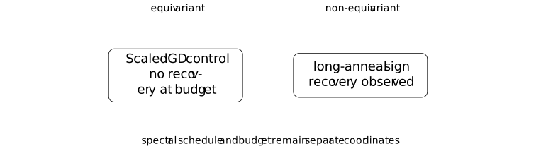
The controls are reported in Remark 4.7 and Appendix D.10 of The loss does not see the basis, but Adam does[singh2026lossbasis]. The source reports no tuned reproducibility baseline for the ScaledGD control. The diagram is not a convergence theorem.

4. Optimizer geometry in training interventions [ftip-00BS]

Equivalent parameterizations need not follow equivalent training trajectories. Their evolution also depends on the update geometry; the scalar loss and represented starting object do not always suffice.

Definition 4.1. Objective-equivalent parameterizations [ftip-00BT]

Two factor pairs $(U,V)$ and $(\widetilde U,\widetilde V)$ are objective-equivalent for $L=f\circ W$ when

\[ W(U,V)=W(\widetilde U,\widetilde V). \]

They then have the same scalar loss for every objective depending only on that represented matrix. Orthogonal gauge-related pairs are objective-equivalent by Lemma 1.3; objective equivalence need not imply membership in the same orthogonal orbit.

Definition 4.2. Parameterization-stable training intervention [ftip-00BU]

Fix a factorized objective, an update algorithm, hyperparameter schedule, randomness coupling, stopping rule, and initial optimizer state. The resulting training intervention is parameterization-stable on an orthogonal orbit when every two gauge-related initial states have identical represented trajectories:

\[ \widetilde U_t\widetilde V_t^{\mathsf T}=U_tV_t^{\mathsf T} \qquad \hbox {at every compared step }t. \]

This is a local stability property of a fully declared intervention. It does not say that arbitrary objective-equivalent pairs outside the orbit must agree.

proposition 4.3. Gauge equivariance gives parameterization stability [ftip-00BV]

Every gauge-equivariant optimizer is parameterization-stable on each orthogonal orbit, provided the remaining protocol coordinates are coupled as in Definition 4.2.

Proof.

Definition 1.8 gives $(\widetilde U_t,\widetilde V_t)=(U_tQ,V_tQ)$. Hence

\[ \widetilde U_t\widetilde V_t^{\mathsf T} =U_tQQ^{\mathsf T}V_t^{\mathsf T}=U_tV_t^{\mathsf T}. \]

This is a sufficient condition on a declared orbit, not a claim that equivariance is necessary for every possible equality of represented trajectories.

proposition 4.4. A first-step defect falsifies a loss-only protocol specification [ftip-00BW]

Suppose two orthogonally gauge-related initializations have equal represented object and scalar objective, but a declared update produces different represented objects after one step. Then the training intervention is not determined by the represented initialization and scalar objective alone.

Proof.

If those two objects determined the intervention, equal inputs would give the same represented next state. The witnessed inequality contradicts that factorization.

Proposition proposition 2.8 and Example 2.9 instantiate its premise for one factored quadratic and zero-state Adam. It proves underspecification, not a capability difference.

Example 4.5. The orthogonal gauge of an attention head [ftip-00BX]

For the row-vector attention weights of Definition [ftip-000P], let $W^Q,W^K\in \mathbb R^{d\times d_h}$ and $Q_h=XW^Q$, $K_h=XW^K$. Attention logits depend on these weights through

\[ Q_hK_h^{\mathsf T}=XW^Q(W^K)^{\mathsf T}X^{\mathsf T}. \]

For $A\in \mathrm O(d_h)$, the right action $(W^Q,W^K)\mapsto (W^QA,W^KA)$ preserves the middle product.

$\text{[math]}$

Section 6 of The loss does not see the basis, but Adam does[singh2026lossbasis] uses column-vector weights and the invariant $W_Q^{\mathsf T}W_K$. Transposition gives the row-vector invariant $W^Q(W^K)^{\mathsf T}$, with the action on the right as displayed.

Remark 4.6. What the attention-twin experiment observes [ftip-00BY]

Section 6 and Table 3 of The loss does not see the basis, but Adam does[singh2026lossbasis] compare two function-equivalent initializations of a two-layer, four-head transformer on modular addition. The reported relative logit distance after one Adam step is $3.6\times 10^{-3}$, versus $2.9\times 10^{-7}$ for a same-basis noise twin; the final per-head invariant distance is reported as 56 percent.

The exact first-step defect has an algebraic explanation, but later drift, scale robustness, and downstream behavior are empirical. The tested small transformers, precision, optimizer allocation, seeds, and task do not establish a frontier-wide law.

Example 4.7. One loss quotient and two optimizer trajectories [ftip-00BZ]

A loss-only description collapses a gauge orbit to one represented starting point. A basis-sensitive optimizer can split that quotient back into different represented trajectories.

$\text{[math]}$

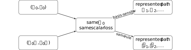
The right-hand split is possible only because the centre box omits the factor basis and optimizer geometry. An FTIP admissible protocol in Definition [ftip-005J] must retain those intervention coordinates when they affect the executable result.

Remark 4.8. Product symmetry and the scope of optimizer conclusions [ftip-00C0]

The relevant optimizer results appear in version 1 of [⧉], submitted 5 August 2026: Sections 3--4 and 6, Appendices B.1--B.6 and B.9, with limitations in Section 11.

The full product symmetry acts on the factors by

\[ (U,V)\longmapsto (UA,VA^{-\mathsf T}). \]

It does not use $(UA,VA)$. For row-vector attention weights, the corresponding action uses right multiplication, as in Example 4.5.

The general rectangular preconditioner representation need not have the square-case uniqueness. A probability-one full-rank claim additionally needs a law for the gradient; a generic full-rank observation does not specify one.

The coordinatewise theorem is a zero-state, memoryless obstruction. The clock theorem is continuous-time and excludes scalar-Adam's momentum. Experimental optimizer and attention results remain observations reported by the source. Equivariance is not identified with low-rank recovery.

Remark 4.9. Continuous-flow conclusions and discrete optimization [ftip-00C1]

The factored-model results prove that update geometry can be a genuine intervention coordinate even when objective and represented initialization are fixed. They do not prove transformer or RLVR convergence, practical optimizer superiority, a scaling law, or any change in reliable capability. Different represented trajectories are not by themselves an acquisition witness of Definition [ftip-005X].

The memoryless theorem does not describe Adam's full state, and the continuous-flow result does not supply discrete rates or finite-step bounds. The source also notes that fixed-rank LoRA changes the learned-rank mechanism; no LoRA transfer is made here.

A dynamic-compute comparison also depends on active research state, persistent harness state, retained history, evaluation configuration, and descendant and retry costs. One realized chain and an archive-best envelope are different outcomes, even at the same declared budget.

References

Reference. The loss does not see the basis, but Adam does [singh2026lossbasis]

@article{singh2026lossbasis,
  title = {The Loss Does Not See the Basis, but Adam Does},
  author = {Singh, Devender},
  year = {2026},
  url = {https://arxiv.org/abs/2608.05136v1},
  journal = {arXiv preprint arXiv:2608.05136}
}

Reference. Towards resolving the implicit bias of gradient descent for matrix factorization: Greedy low-rank learning [li2021greedy]

2021
Zhiyuan Li, Yuping Luo, Kaifeng Lyu
https://arxiv.org/abs/2012.09839v1

@inproceedings{li2021greedy,
  title = {Towards Resolving the Implicit Bias of Gradient Descent for Matrix Factorization: Greedy Low-Rank Learning},
  author = {Li, Zhiyuan and Luo, Yuping and Lyu, Kaifeng},
  booktitle = {International Conference on Learning Representations},
  year = {2021},
  url = {https://arxiv.org/abs/2012.09839v1}
}

Reference. Implicit regularization in deep matrix factorization [arora2019implicit]

2019
Sanjeev Arora, Nadav Cohen, Wei Hu, Yuping Luo
https://arxiv.org/abs/1905.13655v1

@inproceedings{arora2019implicit,
  title = {Implicit Regularization in Deep Matrix Factorization},
  author = {Arora, Sanjeev and Cohen, Nadav and Hu, Wei and Luo, Yuping},
  booktitle = {Advances in Neural Information Processing Systems},
  year = {2019},
  url = {https://arxiv.org/abs/1905.13655v1}
}

Reference. Implicit regularization in matrix factorization [gunasekar2017implicit]

2017
Suriya Gunasekar, Blake Woodworth, Srinadh Bhojanapalli, Behnam Neyshabur, Nathan Srebro
https://arxiv.org/abs/1705.09280v1

@inproceedings{gunasekar2017implicit,
  title = {Implicit Regularization in Matrix Factorization},
  author = {Gunasekar, Suriya and Woodworth, Blake and Bhojanapalli, Srinadh and Neyshabur, Behnam and Srebro, Nathan},
  booktitle = {Advances in Neural Information Processing Systems},
  year = {2017},
  url = {https://arxiv.org/abs/1705.09280v1}
}

Context

Architecture-conditioned potential and computation [ftip-00JC]

This chapter refines the evaluation framework for claims that depend on architecture, optimization geometry or a systems implementation. It begins with the decoder-only Transformer, then introduces architecture-indexed frontiers and matched-compute comparisons, and studies how an optimizer can depend on the representation of its parameters.

The reference architecture specifies how token probabilities are computed; it does not replace the shared task and evaluation interfaces. Readers whose question does not depend on an architecture or optimizer can continue directly to conceptual discovery. Changes to retained context and rollout computation are treated with agent state.

Decoder-only Transformer architecture [ftip-000K]

The continuation law in Definition [ftip-000I] specifies what probabilities a language model exposes. A decoder-only Transformer specifies how a sequence of token identifiers is transformed into those probabilities. This section introduces one component at a time, with dimensions fixed before the component formulas are used.

Notation. Tensor dimensions, positions, heads, and layers [ftip-000L]

Let $T$ be the maximum token positions processed together, $d$ the residual-stream width, $d_{\mathrm {ff}}$ a feed-forward hidden width, $H$ the number of attention heads, $d_h$ the query-key width of one head, and $L$ the number of decoder layers. Positions are indexed by $t,s\in \{1,\ldots ,T\}$, heads by $h\in \{1,\ldots ,H\}$, and layers by $\ell \in \{1,\ldots ,L\}$.

A batch of $B$ hidden-state sequences is a tensor in $\mathbb R^{B\times T\times d}$. When the batch coordinate is irrelevant, write $X\in \mathbb R^{T\times d}$ and let $X_t\in \mathbb R^d$ denote its row at position $t$. Matrix products act on the final coordinate.

Definition. Token embedding [vaswani2017attention, sec. 3.4, Embeddings and Softmax] [ftip-000M]

Let $\mathcal V$ be the vocabulary of Definition [ftip-000D] and $d$ the residual width of Notation [ftip-000L]. A token embedding matrix is a learned matrix $E\in \mathbb R^{|\mathcal V|\times d}$. The hidden vector assigned to token $a\in \mathcal V$ is the row $E_a\in \mathbb R^d$.

For a sequence $x_{1:n}$, embedding lookup produces the matrix $X^{\mathrm {tok}}\in \mathbb R^{n\times d}$ with row $X^{\mathrm {tok}}_t=E_{x_t}$. This operation maps token identifiers to vectors; it does not yet encode their positions.

Definition. Embedding-stage positional transformation [ftip-000N]

Using the dimensions of Notation [ftip-000L], an embedding-stage positional transformation is a specified family of position-dependent transformations $r_t:\mathbb R^d\to \mathbb R^d$, one for each $t\in \{1,\ldots ,T\}$. Applied after the token embedding of Definition [ftip-000M], it produces the initial hidden vector \[ X^{(0)}_t=r_t(E_{x_t}). \] The family $(r_t)_{t=1}^T$ is part of the architecture, even when it has no learned parameters.

Remark. Where positional information enters [ftip-000O]

Definition [ftip-000N] covers only mechanisms acting on the hidden vector at the embedding stage. The original Transformer adds a fixed or learned vector $p_t$ to the token embedding, so $r_t(z)=z+p_t$; see [vaswani2017attention, §3.5].

Relative-bias methods instead alter an attention score as a function of the displacement $t-s$. ALiBi gives one such construction in [press2021train, §3].

Rotary position embedding applies position-indexed rotations to queries and keys rather than adding a vector to the residual stream; see RoFormer, Section 3.2, equations (14)--(16) [⧉]. These mechanisms are not interchangeable choices of one tensor: they act at different points in the computation, so a model specification must name the mechanism and placement.

Definition. Query, key, and value projections [vaswani2017attention, sec. 3.2.1] [ftip-000P]

Let $X\in \mathbb R^{T\times d}$ use the notation of Notation [ftip-000L]. For attention head $h$, choose learned matrices \[ W_h^Q,W_h^K\in \mathbb R^{d\times d_h}, \qquad W_h^V\in \mathbb R^{d\times d_v}, \] where $d_v$ is the value width of one head. The query, key, and value matrices are \[ Q_h=XW_h^Q,\qquad K_h=XW_h^K,\qquad V_h=XW_h^V. \] Their rows associate a query, key, and value vector with each token position.

Definition. Scaled dot-product attention [vaswani2017attention, sec. 3.2.1, equation (1)] [ftip-000Q]

Using the head widths in Definition [ftip-000P], let $T_q,T_k\geq 1$ be query and key-value sequence lengths. For $Q\in \mathbb R^{T_q\times d_h}$, $K\in \mathbb R^{T_k\times d_h}$, and $V\in \mathbb R^{T_k\times d_v}$, scaled dot-product attention is \[ \operatorname {Att}(Q,K,V) =\operatorname {softmax}\left (\frac {QK^{\mathsf T}}{\sqrt {d_h}}\right )V. \] The softmax is applied across each row of the $T_q\times T_k$ score matrix, so every output row is a convex combination of the value rows.

Example. A two-token attention calculation [ftip-000R]

A scalar attention head on two positions makes the masked softmax and its resulting value average explicit.

$\text{[math]}$

Take head width $d_h=1$, so the scale $1/\sqrt {d_h}$ is one. At position two both keys are causally available. Therefore \[ \operatorname {softmax}(0,\log 3) =\frac {(1,3)}{1+3} =\left (\tfrac 14,\tfrac 34\right ), \qquad z_2=\tfrac 14\cdot 2+\tfrac 34\cdot 6=5. \]

Substitution into the scaled dot-product attention of Definition [ftip-000Q] produces the displayed value. Projection matrices, multiple heads, normalization, and residual connections remain outside this scalar calculation; it represents only one attention operation.

Definition. Causal attention mask [vaswani2017attention, sec. 3.2.3] [ftip-000S]

For a length-$T$ sequence, the causal attention mask is the matrix $M\in (\mathbb R\cup \{-\infty \})^{T\times T}$ with \[ M_{ts}= \begin {cases} 0,&s\leq t,\\ -\infty ,&s>t. \end {cases} \] Masked self-attention replaces the score matrix in Definition [ftip-000Q] by $QK^{\mathsf T}/\sqrt {d_h}+M$. Consequently, the output at position $t$ has zero attention weight on every later position $s>t$.

Example. A length-four causal mask [ftip-000T]

For four positions, a causal mask admits the current and earlier keys and excludes every future key.

$\text{[math]}$

Rows index querying positions and columns index key positions. In row three, the first three entries remain available and the fourth receives $-\infty $; after softmax the fourth token therefore contributes exactly zero.

The construction is the autoregressive mask of [vaswani2017attention, Section 3.2.3]. It enforces a dependency restriction. Effective use of the available earlier positions is a separate model property.

Definition. Multi-head self-attention [vaswani2017attention, sec. 3.2.2] [ftip-000U]

For each head $h\in \{1,\ldots ,H\}$, form $Q_h,K_h,V_h$ as in Definition [ftip-000P] from the same input $X$, and apply the masked attention of Definition [ftip-000S]: \[ Z_h=\operatorname {softmax}\left ( \frac {Q_hK_h^{\mathsf T}}{\sqrt {d_h}}+M \right )V_h. \] With $W^O\in \mathbb R^{H d_v\times d}$, multi-head self-attention is \[ \operatorname {MHA}(X) =\operatorname {Concat}(Z_1,\ldots ,Z_H)W^O. \] It returns one width-$d$ vector at every input position.

Remark. Multi-head, grouped-query, and compressed-attention variants [ftip-000V]

The multi-head construction in Definition [ftip-000U] stores a key and value projection per query head. Grouped-query attention instead partitions query heads into groups that share key and value heads; see Ainslie et al., Section 2 [⧉]. This changes parameter and cache shapes while preserving the query-key-value semantics.

Multi-head latent attention first compresses key-value information through a lower-dimensional latent representation and reconstructs head-specific quantities; see DeepSeek-V2, Section 2.1 [⧉]. DeepSeek-V3, Section 2.1, records a later use of that architecture [⧉]. These architectural differences do not establish that their post-training effects equal those of ordinary multi-head attention.

Definition. Positionwise feed-forward sublayer [vaswani2017attention, sec. 3.3, equation (2)] [ftip-000W]

With widths $d$ and $d_{\mathrm {ff}}$ from Notation [ftip-000L], a positionwise feed-forward sublayer is a map $F:\mathbb R^d\to \mathbb R^d$ of the form \[ F(z)=\phi (zW_1+b_1)W_2+b_2, \] where $W_1\in \mathbb R^{d\times d_{\mathrm {ff}}}$, $W_2\in \mathbb R^{d_{\mathrm {ff}}\times d}$, the vectors $b_1,b_2$ have the corresponding widths, and $\phi $ is applied coordinatewise. The same map is applied independently at each token position.

Definition. Sparse mixture-of-experts routing [ftip-000X]

Let $J\geq 1$ and $1\leq k\leq J$. Let $F_1,\ldots ,F_J:\mathbb R^d\to \mathbb R^d$ be feed-forward experts and let $g:\mathbb R^d\to \mathbb R^J$ be a router. For a hidden vector $z$, let $S_k(z)$ be the indices of the $k$ largest coordinates of $g(z)$, breaking equal scores by a fixed total order on expert indices. A sparse mixture-of-experts layer returns \[ F_{\mathrm {MoE}}(z) =\sum _{j\in S_k(z)}\alpha _j(z)F_j(z), \qquad \alpha _j(z)= \frac {\exp g_j(z)}{\sum _{i\in S_k(z)}\exp g_i(z)}. \] Only the selected experts are evaluated for that token.

Remark. Dense and routed feed-forward computation [ftip-000Y]

The dense sublayer in Definition [ftip-000W] evaluates one learned map for every token. The sparsely gated construction of Shazeer et al., Section 2, selects among multiple experts and introduces an additional routing and load-balancing problem [⧉]. The top-$k$ selection rule is described in Definition [ftip-000X].

Parameter count, active parameter count, and executed operations therefore need not agree. A post-training comparison involving routed models must state which quantity is held fixed and whether the router itself is updated.

Example. Top-k expert routing and its DeepSeek counterpart [ftip-000Z]

A routed mixture-of-experts layer uses router scores to activate only a declared subset of routed experts, then combines their outputs with any shared expert path.

$\text{[math]}$

The revision-pinned configuration [⧉] declares $256$ routed experts, $6$ experts selected per token, and one shared expert. This instantiates the selection interface while leaving the artifact's router scores, load-balancing mechanism, and expert outputs unspecified.

Definition. Residual connection [vaswani2017attention, sec. 3.1] [ftip-0010]

Using the sequence and residual dimensions of Notation [ftip-000L], let $F:\mathbb R^{T\times d}\to \mathbb R^{T\times d}$ be a sublayer whose input and output have the same shape. A residual connection forms \[ R_F(X)=X+F(X). \] The addition is coordinatewise. Shape equality is part of the construction; the residual path is not a concatenation of features.

Definition. Layer normalization [ba2016layer, sec. 3] [ftip-0011]

For the residual width $d$ of Notation [ftip-000L], a declared numerical stabilizer $\varepsilon _{\mathrm {LN}}>0$, and $z=(z_1,\ldots ,z_d)\in \mathbb R^d$, define $\mu (z)=d^{-1}\sum _i z_i$ and $\sigma ^2(z)=d^{-1}\sum _i(z_i-\mu (z))^2$. With learned vectors $\gamma ,\beta \in \mathbb R^d$, layer normalization is \[ \operatorname {LN}(z) =\gamma \odot \frac {z-\mu (z)\mathbf 1} {\sqrt {\sigma ^2(z)+\varepsilon _{\mathrm {LN}}}}+\beta . \] It is applied independently to the hidden vector at each token position. The declared stabilizer makes the numerical operator total on $\mathbb R^d$; the unstabilized expression is recovered where $\sigma ^2(z)>0$ by setting $\varepsilon _{\mathrm {LN}}=0$.

Definition. Normalization placement [ftip-006E]

For a residual stream $X$, a sublayer $F$, and a normalization operator $N$, post-normalization applies $N(X+F(X))$. In pre-normalization, the sublayer receives a normalized input and the residual update is $X+F(N(X))$.

Placement is an architecture coordinate, separate from the formula for $N$. Every decoder block must state which residual branches use which placement.

Definition. Root mean square layer normalization [zhang2019root, Section 4, equation (4)] [ftip-006F]

For $z\in \mathbb R^d$, learned scale $\gamma \in \mathbb R^d$, and a declared numerical stabilizer $\varepsilon _{\mathrm {RMS}}>0$, root mean square layer normalization is

\[ \operatorname {RMSNorm}(z) =\gamma \odot \frac {z}{\sqrt {d^{-1}\sum _{i=1}^{d}z_i^2+ \varepsilon _{\mathrm {RMS}}}}. \]

Unlike layer normalization in Definition [ftip-0011], this operator does not subtract the coordinate mean. The declared stabilizer makes it total at the zero vector; setting the stabilizer to zero recovers the source expression on nonzero inputs.

Remark. Normalization operator and placement are separate choices [ftip-006G]

Ba et al. define layer normalization in [ba2016layer, Section 3]. The original Transformer applies it after residual addition in [vaswani2017attention, Section 3.1]. Xiong et al. distinguish post-normalized and pre-normalized Transformers in [xiong2020layer, Section 3.3]. Either the normalization operator or its placement can change while the other is held fixed.

A later stability statement must therefore name both choices. A result about the normalization formula alone does not determine the residual path.

Definition. Decoder-only Transformer language model [phuong2022formal, sec. 6, Decoder-only transformers] [ftip-0012]

A decoder-only Transformer language model consists of:

the token interface in Definition [ftip-000E];
an initial representation from Definition [ftip-000M] and Definition [ftip-000N];
a stack of $L$ causal decoder layers built from the attention, feed-forward, residual, and normalization constructions in Definition [ftip-000S]--Definition [ftip-0011]; and
an output map from the final hidden vector to token logits.

If the final hidden vector at position $t$ is $h_t\in \mathbb R^d$, an output matrix $W_U\in \mathbb R^{|\mathcal V|\times d}$ and bias $b_U\in \mathbb R^{|\mathcal V|}$ give logits $z_t=W_Uh_t+b_U$. The softmax \[ \pi _\theta (a\mid x_{1:t}) =\frac {\exp (z_{t,a})} {\sum _{v\in \mathcal V}\exp (z_{t,v})} \] realizes the conditional next-token law of Definition [ftip-000H]. The parameter tuple $\theta $ contains every learned tensor named by this architecture.

Example. Decoder-only dataflow and a DeepSeek V4-Flash provenance overlay [ftip-0013]

A decoder pipeline maps token identifiers through hidden states to logits; the released model instance and family report provide different evidence about that pipeline.

$\text{[math]}$

The pinned configuration [⧉] declares 43 layers, hidden width 4096, 64 attention heads, and one key--value head. Section 2 of the family report [⧉] describes the preview architecture. Neither source identifies a complete 0731-specific architecture or training delta. The diagram records the interface, not a small copy of the released model.

Architecture-indexed ceilings and matched compute [ftip-00JF]

This optional section refines the architecture-neutral capability framework only when the question names an architecture, optimizer, or systems implementation. The general model/interface formulation remains available when these fields are unnecessary.

Architecture comparisons below are conditional on a declared task family, evaluation law, intervention class, and scalar cost. Toy bounds are finite results under their displayed assumptions and do not transfer to concrete model instances without verified interface, task, and cost assumptions.

Architecture, optimizer, and systems variables [ftip-00JG]

Architecture, optimizer, and systems fields refine the model/interface description. A comparison depends only on the fields named in its assumptions and conclusion.

Definition. Optional architecture refinement [ftip-00JH]

Let $M$ denote an existing model intervention. An architecture refinement is a record $A=(\mathcal X,\mathcal Y,\operatorname {Map}_A)$ whose map realizes the same declared input and output interface. Forgetting $A$ returns $M$; no architecture claim is made when the field is omitted.

Definition. Optimizer and systems records [ftip-00JI]

When needed, extend the record by $O$ for optimizer and state-update rules, and $S$ for kernels, precision, memory, cache, and scheduling. The triplet $(A,O,S)$ is descriptive; it is not a scalar intelligence score.

Definition. Architecture-indexed evaluation functional [ftip-00JJ]

Fix an architecture $A$, its base artifact, a declared intervention set $\mathfrak I_A$, and the common evaluation interface of Convention [ftip-005D]. Each $\eta \in \mathfrak I_A$ specifies a protocol $P_{A,\eta }=\operatorname {PostTrain}(A,\eta )$ in that measurable and absolutely integrable evaluation domain, with real performance $J_{\rm ev}(P_{A,\eta })$. Let $c_A(\eta )\in [0,+\infty ]$ be its scalar cost under the study's declared accounting rule: a fixed measured cost or an expected nonnegative cost, as specified. For a finite budget $C\in \mathbb R_{\geq 0}$, define \[ V_A(C)=\sup \left \{ J_{\rm ev}(P_{A,\eta }): \eta \in \mathfrak I_A,\ c_A(\eta )\leq C \right \}\in \overline {\mathbb R}. \] Infinite-cost interventions are infeasible at every such budget.

As in Definition [ftip-005M], the empty feasible set has value $-\infty $; an unbounded-above feasible score set has value $+\infty $. The value is real exactly when that set is nonempty and bounded above. Increasing $C$ enlarges the feasible set, so $V_A$ is nondecreasing. A finite supremum need not be attained by any intervention.

Frontier differences and derivatives are ordinary real operations only where the relevant values are finite, with differentiability additionally required for a derivative. Cost ratios use the domain in Definition [ftip-00JP]. The allowed intervention set, evaluation law, and accounting rule are part of the definition, so $V_A$ is not a universal intelligence function.

Remark. Architecture-neutral projection and gradual complexity [ftip-00JK]

A statement that depends only on the model/interface map is invariant under changes to architecture $A$, optimizer $O$, or systems $S$ that leave that map fixed. A conclusion about one of those fields instead requires assumptions that distinguish its possible values.

Definition. Three ceiling layers [ftip-00JL]

For fixed task and evaluation laws, distinguish the representational ceiling of $A$, the optimizer-reachable ceiling of $(A,O)$, and the systems-feasible frontier of $(A,O,S,C)$. Each layer is conditional on the objects named; none implies that the next layer attains it.

Remark. Architecture effects are comparative estimands [ftip-00JM]

A difference between two architectures is meaningful only after the task, data, post-training, inference, evaluation, and cost records identify which coordinates are held fixed and which are allowed to vary.

Depth reuse and latent recurrence [ftip-00KG]

Repeated depth, latent feedback, and recirculation change the computation performed at inference. Relative to the fixed reference autoregressive Transformer, their costs include any extra passes, state, and prefill work.

Definition. Computation-axis record [ftip-00KH]

For an architecture record $A$, distinguish token steps, feed-forward depth passes, recurrent passes, and latent-state updates. Let $d(A,r)$ be the declared number of depth passes in run $r$; it is a computation coordinate, not a synonym for parameter count or reasoning quality.

Remark. Looped Transformers as a source result [ftip-00KI]

Giannou et al. show that a fixed shallow Transformer placed in a loop can execute programmed iterative computations, including conditional branches and in-context algorithms, in Looped Transformers as Programmable Computers[giannou2023looped]. This is a source result under its program, state, and precision assumptions; it is not a universal claim about language-model capability.

Remark. Parameter sharing and width tradeoffs [ftip-00KJ]

Xue et al. report that depth sharing can reduce trainable parameters while limiting modeling capacity, and study width and mixture-of-experts remedies in Go Wider Instead of Deeper[xue2021wider]. The comparison is empirical and task-specific; it does not identify a depth-independent ceiling.

Remark. Virtual logical depth and scaling [ftip-00KK]

Zhu et al. vary virtual logical depth by reusing weights and report reasoning gains at nearly fixed parameter count in Beyond Parameters: Exploring Virtual Logic Depth for Scaling Laws[zhu2025virtualdepth]. Their results motivate a depth coordinate in a scaling study, while leaving knowledge capacity, optimization, and transfer dependent on the declared training and evaluation protocol.

Remark. Recirculation as an inference intervention [ftip-00KL]

Mozer et al. introduce inference-time recirculation that feeds latent states back through an off-the-shelf model and report task improvements in Recirculation[mozer2026recirculation]. The added serial prefill and adaptive tuning belong in the systems and inference records; the observation is not a proof of a new representational ceiling.

Remark. Latent feedback with a preserved Transformer interface [ftip-00KM]

Wang et al. widen the feedback channel between decoding steps with latent feedback while retaining a Transformer and language-modeling interface in Full-bandwidth transformer[wang2026fullbandwidth]. Any reported token or accuracy savings are conditional on the scheduled multi-pass training and measured decoding cost.

Remark. Latent prediction as a training intervention [ftip-00KN]

Teoh et al. add next-latent prediction to next-token training and report compact predictive states without changing the Transformer interface in Next-Latent Prediction Transformers Learn Compact World Models[teoh2025nextlatent]. This belongs to the training intervention record, not to an architecture-only comparison.

Example. Equal parameters do not fix effective depth [ftip-00KO]

Two runs can share parameter count while using different numbers of recurrent or latent-feedback passes. A matched study must therefore report the computation-axis record and cannot infer an architecture ceiling from parameters alone.

Definition. Depth-reuse model-instance record [ftip-00KP]

For a depth-reuse comparison, record shared weights, pass count, stopping rule, recurrent state, training objective, token and pass FLOPs, prefill and decode latency, memory, and evaluation seeds. A pass-count change is an intervention even when the parameter tensor is unchanged.

Example. Fixed-recipe depth comparison [ftip-00KQ]

In a fixed-recipe arm, hold data, optimizer, feedback, stopping rule, and evaluation law fixed while varying only the declared depth-reuse intervention. The resulting difference is an estimand for that recipe, not a best-achievable comparison.

Remark. Scaling surfaces rather than a single law [ftip-00KR]

A depth-reuse study may fit a surface over parameters, tokens, passes, and cost. The fit is an empirical summary over its measured range; it does not establish an asymptotic law or a universal saturation point.

Remark. Architecture and training are separable records [ftip-00KS]

Weight sharing, latent objectives, and recirculation can alter optimization without changing the declared external interface. The comparison must retain architecture, training intervention, and systems coordinates separately.

Remark. Depth reuse across passes, parameters, and tasks [ftip-00KT]

The cited looped, virtual-depth, latent-feedback, and recirculation results do not show that more passes always improve capability, that parameter sharing dominates added parameters, or that inference-time gains transfer to training or to another task family. Each transfer requires a matched model-instance record.

Ceilings, frontiers, and saturation [ftip-00JN]

Definition. Fixed-recipe and tuned frontiers [ftip-00JO]

The fixed-recipe frontier evaluates one common $\eta $. The equal-tuning frontier permits architecture-specific choices from a predeclared trial set with the same tuning data and budget. The restricted envelope permits a predeclared class of interventions under $C$. These are distinct estimands.

Definition. Iso-quality cost ratio [ftip-00JP]

For a finite real target $q\in \mathbb R$ and the frontier of Definition [ftip-00JJ], define the inverse cost \[ C_A(q)=\inf \{C\in \mathbb R_{\geq 0}:V_A(C)\geq q\} \in [0,+\infty ], \qquad \inf \varnothing =+\infty . \] The iso-quality ratio is defined only on the domain \[ \rho _{A/B}(q)=\frac {C_A(q)}{C_B(q)}, \qquad 0\leq C_A(q)<+\infty , \quad 0<C_B(q)<+\infty . \] The architectures must use the same target, evaluation interface, cost units, and comparison arm. The ratio compares efficiency under these choices.

An inverse cost is a threshold infimum, not an executable minimum. The infimum over budgets may be unattained; even if a budget satisfies $V_A(C)\geq q$, its performance supremum may be unattained at $q$. An actual target-achieving intervention requires a separate witness.

Positive individual costs do not guarantee a positive inverse cost. For interventions $\eta _n$, $n\geq 1$, with score $1$ and cost $1/n$, the target $q=1$ has $C_A(1)=0$, although every intervention costs more than zero. If both architectures have this family, the putative ratio is $0/0$ and is excluded by the displayed domain.

Definition. Operational cost vector and scalarization [ftip-00JQ]

Record training FLOPs, inference FLOPs, wall time, memory, energy, and hardware separately as $\mathbf c$. A scalar cost $C=w\cdot \mathbf c$ is a declared study choice with nonnegative units $w$; changing $w$ changes the frontier and must not be hidden as architecture quality.

Theorem. Finite-window representational obstruction [ftip-00JR]

Consider a causal system whose state after each prefix has at most $K$ distinct values, and a task with $K+1$ prefixes requiring pairwise distinct continuation labels. By the pigeonhole principle two prefixes share a state, so at least one continuation label is wrong. This is a finite toy obstruction only; it does not bound a concrete Transformer or KDA instance without a proved reduction to this state model.

Theorem. A conditional saturation certificate [ftip-00JS]

Let $V_A$ be the nondecreasing frontier of Definition [ftip-00JJ], bounded above by a finite $U\in \mathbb R$. If an intervention reaches a real target $q<U$ at a finite cost $C_q\geq 0$, then at every finite $C\geq C_q$, $q\leq V_A(C)\leq U$. In particular $V_A(C)$ is real and $0\leq U-V_A(C)\leq U-q$. This elementary certificate is conditional on the bound $U$; it does not assert that real intelligence saturates.

Example. Equal scalar cost does not identify architecture [ftip-00JT]

Two systems can have the same scalar $C$ while differing in memory, latency, and training allocation. A cost-weight change can reverse their ordering without changing either system. Thus a one-factor comparison needs a fixed scalarization and a reported cost vector; no architecture effect follows from equal $C$ alone.

Matched-compute comparison protocol [ftip-00JU]

Definition. Common-recipe comparison arm [ftip-00JV]

A common-recipe arm fixes training data, optimizer family, schedule, post-training procedure and feedback, training and post-training budgets, inference budget, and evaluation protocol and draws. Interface-compatible parameter choices are declared in advance as part of each permitted architecture package. The comparison varies that package under the common recipe; any further deviation is recorded as a separate comparison coordinate. Its score difference measures performance under this recipe, not the best attainable result for either architecture.

Definition. Equal-tuning-budget comparison arm [ftip-00JW]

An equal-tuning-budget arm permits architecture-specific tuning under a predeclared protocol that fixes the tuning data and its volume, trial count, selection rule, stopping rule, and tuning cost for both architectures. The cost uses the same declared accounting rule. The resulting comparison measures practical performance under this equal optimization effort; it does not determine best possible training or a representation-only limit.

Definition. Restricted-envelope comparison arm [ftip-00JX]

A restricted-envelope arm declares an allowed intervention class $\mathcal E_A\subseteq \mathfrak I_A$ for each architecture, specifying the permitted training, post-training, and inference procedures. The classes expose exclusions, search budgets, seeds, and stopping rules. Restrict the evaluation functional of Definition [ftip-00JJ] to $\mathcal E_A$ and compare the resulting suprema under the same finite cost cap $C\geq 0$, common evaluation law, and common declared cost accounting.

The measurable, integrable evaluation domain and extended-real conventions of Definition [ftip-00JJ] apply: an empty feasible class has value $-\infty $, an unbounded-above feasible score set has value $+\infty $, and a finite supremum need not be attained. The allowed class is part of the comparison, so its envelope is a restriction-dependent quantity, not an unrestricted architectural ceiling.

Definition. Model-instance comparison evidence record [ftip-00JY]

A model-instance record contains architecture/checkpoint identity, parameter count, data and post-training recipe, optimizer, precision, hardware, cache policy, training and inference cost vectors, task suite, and independent evaluation seed. A missing field makes an architecture attribution unknown.

Remark. Systems optimizations are measured interventions [ftip-00JZ]

FlashAttention, KV-cache layouts, quantization, batching, and kernels can change feasible cost. If they approximate, truncate, or alter precision of the mathematical computation, the record must mark that as a systems intervention rather than as a pure architecture comparison.

Theorem. Matched-protocol difference is an estimand [ftip-00K0]

Given $n\geq 1$ evaluation draws, let $\widehat V_A(C)$ be the sample mean of finite real evaluation scores for architecture $A$ at a finite cost cap $C\geq 0$. Under a fixed evaluation law and common-recipe arm, the finite difference $\widehat V_A(C)-\widehat V_B(C)$ is a well-defined empirical estimand.

It does not identify a causal architecture effect when data, tuning, or systems coordinates differ. The conclusion follows directly from the declared record.

Remark. Conditions for applying a toy model [ftip-00K1]

A toy theorem applies to a concrete model only if an explicit map from its state and interface to the model preserves the theorem's assumptions, including its cost accounting. Without such a map, the conclusion concerns only the abstract model; its validity for the concrete system is unknown.

Kimi Delta Attention versus Transformer [ftip-00K2]

Definition. KDA model-instance record [ftip-00K3]

For a Kimi Delta Attention (KDA) versus full-attention baseline study, record the exact Kimi Linear checkpoint, layer mix, context length, hardware, kernel, precision, batch, and decoding workload. The paper describes KDA as a fine-grained gated delta-rule module in a hybrid architecture; those are source observations from Kimi Linear: An Expressive, Efficient Attention Architecture[kimi2025linear], not universal theorems.

If the baseline is called a Transformer, record whether it is the paper's MLA baseline or another full-attention implementation; the label alone does not identify a common architecture or cost.

Example. Matched-cost KDA and Transformer comparison [ftip-00K4]

A matched comparison uses the same task prompts, post-training data and feedback, optimizer family, evaluation protocol, and quality target. The corresponding measurements include parameter count, training FLOPs, inference FLOPs, wall time, memory, KV-cache bytes, and context length for each architecture. A reported speed or quality difference is conditional on these experimental conditions and measurements.

Remark. What the Kimi Linear paper establishes [ftip-00K5]

Kimi Linear reports a hybrid KDA/MLA model and fair-comparison experiments in Sections 3--5, with setup in Section 5.4 and efficiency comparisons in Sections 5.5--5.6 of Kimi Linear: An Expressive, Efficient Attention Architecture[kimi2025linear]. These include long-context efficiency.

The reported throughput and quality are empirical under its training recipe and hardware; they are lower bounds on demonstrated performance, not an architecture-independent ceiling.

Example. Parameter matching is not cost matching [ftip-00K6]

Two models with equal parameter count can have different attention FLOPs, KV-cache memory, kernel utilization, and attainable context. Conversely, equal wall time can hide different hardware and precision. Therefore a parameter-matched result cannot by itself identify a compute frontier.

Remark. Cache, throughput, and quality in KDA comparisons [ftip-00K7]

The KDA example does not prove that every linear-attention model beats every Transformer, that cache savings imply equal quality, or that a measured throughput gain is a capability gain. Any such statement requires a new matched study with the evidence record of Definition [ftip-00JY].

Definition. Model-instance comparison decision rule [ftip-00K8]

Call architecture A more cost-efficient than B at quality $q$ only when the compared threshold costs use the same declared protocol, the confidence procedure and stopping rule are fixed, and all cost-vector coordinates needed by the claim are present. A ratio additionally requires finite costs and a strictly positive denominator as in Definition [ftip-00JP]. State whether the costs are measured target-achieving witnesses or justified inverse-frontier values $C_A(q)$ and $C_B(q)$; observing one successful run does not identify those infima. Otherwise the comparison is descriptive or unknown.

Interface boundaries for alternative architectures [ftip-00K9]

Definition. JEPA comparability interface [ftip-00KA]

A JEPA-like architecture is comparable to an autoregressive model only after fixing the predictor, target representation, decoder or downstream interface, training objective, inference procedure, and evaluation law. A parameter-count match alone is not a typed comparison.

Remark. Representation and task interface are separate [ftip-00KB]

A latent predictor can be excellent under one decoder and unusable under another. The evaluation record must therefore include the interface that maps the representation to the declared task output.

Theorem. Interface-preserving architecture reduction [ftip-00KC]

If two architecture records induce the same conditional output law on a fixed task and evaluation interface, every evaluation functional $J$ gives the same value. This is an immediate pushforward identity under the stated output-law and interface assumptions. It does not imply that distinct architectures are generally equivalent.

Example. Equal benchmark score can hide different ceilings [ftip-00KD]

Two architectures may tie on a finite benchmark while differing on an unmeasured task slice or longer context. Thus a single score cannot establish equal representational ceilings; the task family and evaluation coverage must be declared.

Remark. Architecture-independent model interfaces [ftip-00KE]

A result stated solely in terms of a model/interface map applies to every architecture realizing that map and satisfying its hypotheses. An architecture-specific conclusion can require further assumptions, as in Remark [ftip-00JK].

Remark. Open model-instance questions [ftip-00KF]

The relative capability and cost of KDA, full attention, and JEPA candidates remain empirical questions. A reproducible comparison requires identified checkpoints or reproducible training, fixed evaluation seeds, and measured cost vectors. Architecture-specific ceilings remain estimands and hypotheses rather than established constants.

Published hybrid-attention comparison [ftip-00KU]

Kimi Linear combines recurrent KDA layers with periodic full MLA attention. Its published comparison shows task-dependent score changes and lower long-context decoding times. The selected scores in Example [ftip-00LC], the memory estimate in Example [ftip-00KY], and the discovery calculation in Example [ftip-00L3] connect these observations to a post-training question: when can a cheaper attempt compensate for a possible lower per-attempt success probability?

Example. Published Kimi Linear operating point [ftip-00KV]

The Kimi Linear report compares experimental models pretrained on 1.4 trillion tokens, each with 48 billion total and 3 billion active parameters. Kimi Linear uses three Kimi Delta Attention layers for each full Multi-head Latent Attention layer, with no positional encoding (NoPE) in its MLA layers; the reference uses full MLA attention [kimi2025linear, Sections 4 and 5.4]. These are properties of the reported hybrid architecture.

These experimental models are distinct from the released Kimi Linear model, pretrained on 5.7 trillion tokens and supporting up to one million tokens of context. Appendix D compares that release with Moonlight, which has 16 billion total and 3 billion active parameters [kimi2025linear, Section 5.4.1 and Appendix D].

Example. Published efficiency observations [ftip-00KW]

For batch size one at one million tokens, Figure 7 labels a $2.9\times $ prefill speedup and a $2.2\times $ decoding speedup for Kimi Linear against MLA. Section 6.3 gives $2.3\times $ for the latter point, so the graphic and prose differ slightly [kimi2025linear, Figure 7 and Sections 5.6 and 6.3].

The larger-batch comparison in Figure 1(b) gives decoding time per output token of 1.84 milliseconds for Kimi Linear and 11.48 milliseconds for MLA, with a reported $6.3\times $ speedup. Section 6.3 describes this as a theoretical speedup from reallocating saved KV-cache memory to larger batches. It illustrates a different use of the memory saving from the batch-one latency result [kimi2025linear, Figure 1(b) and Section 6.3].

Figure 1(a) reports RULER scores of 84.3 for Kimi Linear and 81.3 for MLA at 128k context, with $3.98\times $ decoding acceleration [kimi2025linear, Figure 1(a)]. The report also gives a reduction of up to 75 percent in KV-cache use [kimi2025linear, Abstract]. Together these observations motivate studying context length and batch size as separate cost coordinates. The unequal RULER scores and different timing regimes are retained when interpreting those points.

Definition. Quality target and cost measurement [ftip-00KX]

For a reported benchmark score q, use the same task, prompt law, scoring rule, and post-training condition for both systems. The comparison records the smallest measured cost at which each system reaches q, when such a measurement exists. A throughput or cache ratio is not substituted for this iso-quality cost.

Example. A cache-memory estimate for hybrid attention [ftip-00KY]

The cited FLA KDA implementation at commit 6b6f546f stores one active recurrent state per sequence, with dimensions determined by the value heads and key/value dimensions rather than accumulated context length. Its newly allocated state uses float32 [⧉]. The optional short-convolution state has one fixed-width kernel buffer per channel and sequence [⧉]. This supplies a concrete implementation model for the recurrent part of the 3:1 mixture in Example [ftip-00KV].

Consider a stylized comparison with $4\ell $ layers, batch size $b$, and context length $T$, where $\ell ,b,T$ are positive integers. Assume each MLA layer stores $\kappa T$ bytes per sequence, with the same $\kappa >0$ in both designs, and each KDA layer stores one terminal recurrent-plus-convolution state of $\sigma >0$ bytes. The active attention-state memories are

\[ M_{\rm MLA}=4b\ell \kappa T,\qquad M_{\rm hybrid}=b\ell (\kappa T+3\sigma ),\qquad \frac {M_{\rm hybrid}}{M_{\rm MLA}} =\frac {1}{4}+\frac {3\sigma }{4\kappa T}. \]

The hybrid uses less active state exactly when $T>\frac {\sigma }{\kappa }$, and the ratio tends to $1/4$ as context grows. This explains why replacing three quarters of the growing caches can approach a 75-percent saving, while fixed recurrent-state overhead can erase the advantage at short contexts. The retained MLA layers keep the hybrid's state memory linear in $T$; the whole model is not a fixed-memory recurrent system.

Weights, training activations, workspaces, allocator padding and saved prefix states are outside this active-state calculation. At a fixed device memory budget, the estimate predicts more room for simultaneous or longer rollouts when attention state dominates. It does not predict a fourfold speedup. Training and decoding also use different execution paths: FLA selects chunk kernels for gradient-enabled computation and fused recurrence for short inference calls [⧉]. The fixed-state estimate is therefore a useful serving hypothesis, not a training-memory or training-speed formula.

Example. Common-recipe reading of the Kimi result [ftip-00KZ]

The report holds its stated pretraining and SFT recipes common across the experimental models [kimi2025linear, Sections 5.4--5.5 and Table 4]. The selected observations in Example [ftip-00LC] compare the resulting trained designs, including the hybrid's 3:1 KDA/MLA pattern and NoPE choice. The mixed score directions suggest a task-dependent tradeoff rather than one ordering of the two architectures.

The theoretical mechanism is a change in the cost of maintaining and using the prefix: recurrent layers compress it into state, while the retained MLA layers preserve growing attention caches. The model in Example [ftip-00KY] predicts the largest memory advantage at long contexts. If this advantage reduces the cost of generating useful candidates, Example [ftip-00L3] predicts when more attempts can offset a reduction in per-attempt quality. This is a conditional explanation to test through rollout costs and verified success rates; it does not require attributing the whole result to KDA alone.

Example. Measured iso-quality cost ratio [ftip-00L0]

Let $c_K(q)$ and $c_T(q)$ be measured inference costs for Kimi Linear and the Transformer reference at the same finite real score $q$ and context length, under one accounting rule. If $0\leq c_K(q)<+\infty $ and $0<c_T(q)<+\infty $, the measured ratio $\widehat \rho _{K/T}(q)=c_K(q)/c_T(q)$ is reported together with the full cost vectors. These measured costs need not be the inverse frontier infima of Definition [ftip-00JP]. If either threshold is unmeasured or the denominator is zero, the ratio is left undefined rather than inferred from the paper's speedup plot.

Remark. Hybrid attention is not pure linear attention [ftip-00L1]

Kimi Linear combines KDA with periodic full-attention layers. A measured advantage therefore identifies the reported hybrid intervention, not a claim that a purely linear recurrent architecture has the same quality or ceiling. The layer pattern belongs in the architecture record.

Remark. Demonstrated performance is a lower bound [ftip-00L2]

The published benchmark scores demonstrate attainable points for the reported checkpoints and protocol. They do not establish a representational ceiling, a universal scaling law, or a claim that additional cost cannot improve either architecture.

Example. When cheaper attempts compensate for lower success [ftip-00L3]

Smaller caches can support more concurrent requests or avoid preemption and recomputation. These are actual serving mechanisms in vLLM's memory and scheduling guidance [⧉]. For post-training, the useful prediction is therefore about completed candidate attempts under a budget, including verification and optimization costs, rather than decoding speed alone.

Use the following cost model on the same hardware. One baseline attempt costs $c>0$; generation accounts for a fraction $f\in [0,1]$. Suppose generation becomes $s_{\rm gen}>0$ times as fast while all other cost per attempt stays fixed. The new cost and total attempt-throughput factor are

\[ c_K=c\left (1-f+\frac {f}{s_{\rm gen}}\right ),\qquad S=\frac {c}{c_K} =\frac {1}{1-f+f/s_{\rm gen}}. \]

For a fixed budget $B\geq 0$, this model permits $N_M=\lfloor B/c\rfloor $ baseline attempts and $N_K=\lfloor B/c_K\rfloor $ hybrid attempts. Assume $N_M,N_K\geq 1$ and verified-success events independent within each set of attempts, with respective probabilities $p_M,p_K\in [0,1]$. Then Theorem [ftip-0078] gives discovery probabilities $1-(1-p_M)^{N_M}$ and $1-(1-p_K)^{N_K}$. The hybrid matches or exceeds baseline discovery exactly when

\[ p_K\geq 1-(1-p_M)^{N_M/N_K}. \]

This follows by comparing the two failure probabilities and taking the nonnegative $N_K$-th root.

For an illustrative estimate, suppose generation consumes 80 percent of the baseline cost and use $s_{\rm gen}=2.2$, motivated by the batch-one decode figure in Example [ftip-00KW]. Applying that decode factor to the whole generation stage is a working approximation, not a measured rollout result. Then $S\approx 1.774$; a budget of $B=10c$ buys 10 baseline attempts or 17 hybrid attempts. If $p_M=0.10$ and $p_K=0.08$, the discovery probabilities are approximately $0.651$ and $0.758$. The break-even hybrid probability is about $0.0601$. Thus this model predicts that more attempts can outweigh a moderate per-attempt quality loss. The assumed probabilities are illustrative verified-success rates, not conversions of the benchmark scores in Example [ftip-00LC].

The prediction is strongest for long-context, generation-heavy work whose saved memory becomes usable rollout capacity. As verification or optimization dominates, $f$ shrinks and $S$ approaches one. Correlated attempts require the joint-law analysis of Convention [ftip-0077] instead of the independent product. Measure completed attempts, verified-success rates and total cost under a fixed prompt, decoding and verifier protocol to test the tradeoff. In the RLVR round of Example [ftip-004M], additional successful candidates can improve the available feedback; whether they produce useful accepted updates is a further optimizer-and-evaluation question, as Example [ftip-0085] demonstrates.

Paired measurements for model comparison [ftip-00L4]

A paired measurement specifies both model instances and their task, intervention, evaluation, and cost coordinates. These conditions determine the meaning of each point in the measured frontier.

Definition. Comparison pair identity [ftip-00L5]

A paired comparison identifies the two systems, exact checkpoint or training commit, architecture variant, parameter counts, tokenizer, and context limit. A label such as ``Transformer'' is insufficient when attention, cache, or layer patterns differ.

Definition. Common task and evaluation conditions [ftip-00L6]

Both systems use the same task family, prompt and data law, scoring rule, sampling seeds, stopping rule, and evaluator version. Any exception is a separate comparison arm, not an unrecorded architecture effect.

Definition. Training and post-training coordinates [ftip-00L7]

Record data volume, token order policy, optimizer and schedule, supervised tuning, feedback or reinforcement procedure, update count, and selection rule. The common-recipe arm fixes these coordinates; the equal-tuning arm allows predeclared alternatives with equal search resources.

Definition. Inference and systems coordinates [ftip-00L8]

Record hardware, software and kernel versions, precision, batch, cache policy, sequence lengths, warm-up procedure, concurrency, and decoding settings. A kernel or cache change that alters numerical computation is marked as an intervention rather than hidden as an implementation detail.

Definition. Per-system cost vector [ftip-00L9]

For each system, the cost vector $\mathbf c$ contains training FLOPs, inference FLOPs, wall time, memory, energy when available, and context length. The primary scalar $C$ and its weights are declared beside the vector; omitted coordinates are marked unknown.

Definition. Repeated measurement rule [ftip-00LA]

For each fixed workload and system, record warm-up runs, repetition count, random seeds, and the aggregation rule. Report mean and dispersion for time, memory, and score; a single fastest run cannot define a cost frontier.

Definition. Paired uncertainty estimates [ftip-00LB]

When the same evaluation items are used, report paired score differences and an uncertainty procedure fixed before inspecting the result. Confidence intervals quantify sampling variation; they do not repair unmatched training, systems, or task coordinates.

Example. Published Kimi Linear comparison [ftip-00LC]

Table 4 of the Kimi Linear report compares the experimental models pretrained on 1.4 trillion tokens in Example [ftip-00KV], after the same supervised fine-tuning (SFT) recipe. Both have 48 billion total and 3 billion active parameters. Three selected benchmark scores are [kimi2025linear, Sections 4 and 5.4 and Table 4]:

Arm	MMLU-Pro	LiveBench	EvalPlus
Kimi Linear	67.4	45.2	61.0
Full MLA	65.7	45.7	62.6

The entries use the paper's score units, with larger values better on each selected benchmark; LiveBench is reported as Pass@1. Kimi Linear is higher on MMLU-Pro and lower on LiveBench and EvalPlus in these observations. These are reported point estimates on different tasks, not a single capability score; the table supplies no uncertainty estimate.

The common recipe uses the K2 pretraining corpus, MuonClip and a shared training schedule. SFT proceeds from broad instruction data to targeted reasoning tasks; evaluation uses temperature 1.0 and an internal framework derived from LM-Harness [kimi2025linear, Section 5.4]. Thus the scores provide a concrete example of how the trained hybrid and full-MLA designs respond to the same recipe. The cost mechanism and its possible post-training consequences are developed in Example [ftip-00KZ].

Remark. Measured and assumed costs [ftip-00LD]

A useful cost model can combine measurements with assumptions justified by the architecture and its implementation. In Example [ftip-00L3], the generation share $f$ and speed factor $s_{\rm gen}$ determine a predicted attempt-throughput factor. Their assumed values can be varied without pretending they were measured in the original experiment.

For fixed $f\in [0,1]$, write $S(s)=1/(1-f+f/s)$ for $s>0$. This function is nondecreasing. An interval $s_{\rm gen}\in [s_-,s_+]$, with $0<s_-\leq s_+$, therefore gives the conditional range $S\in [S(s_-),S(s_+)]$. This is sensitivity to a chosen assumption range; it is a statistical confidence interval only if a sampling argument supplies that interpretation.

Definition. Measured contrasts and conditional predictions [ftip-00LE]

A measured paired contrast evaluates the same declared quantity for two observed model instances under a specified task, protocol and cost accounting. The common-recipe scores in Example [ftip-00LC] are one example. A confirmatory comparison fixes its matching and selection rules before examining the scores.

A conditional paired prediction instead uses an explicit model to supply one or more cost or response quantities, then derives the comparison under those assumptions. The discovery probabilities in Example [ftip-00L3] are an example. Such a prediction can be motivated by existing observations and guide a later experiment; its unmeasured inputs remain assumptions, and agreement with new matched measurements tests the model.

Example. How generation share changes the predicted gain [ftip-00LF]

Keep the illustrative generation factor $s_{\rm gen}=2.2$ from Example [ftip-00L3] and vary the baseline generation share $f$. Its cost model gives the following total attempt-throughput factors:

Generation share	Predicted throughput factor
20 percent	1.122
50 percent	1.375
80 percent	1.774
100 percent	2.200

These calculated values show why the same decoding improvement can matter much more for generation-heavy search than for a verifier- or optimizer-dominated workload. They suggest measuring the time spent in generation, verification and updates before selecting where to invest systems effort. A change in the bottleneck changes the useful intervention, even when the attention architecture stays fixed.

Remark. Testing the predicted architecture tradeoff [ftip-00LG]

The memory and discovery models predict the strongest benefit when long prefixes make attention state expensive, saved capacity improves useful rollout throughput, and per-attempt success remains above the break-even threshold. Short contexts, expensive verification, or strongly correlated attempts can weaken that benefit. These are distinct mechanisms to test, rather than a universal ranking of KDA and full attention.

A comparison across implementations can retain this reasoning while re-estimating state sizes, generation share and success probabilities for the new system. Report both the prediction and the matched measurements: their agreement or disagreement identifies which mechanism or assumption needs revision.

Conditional frontier and saturation analysis [ftip-00LH]

A finite matched study measures capability at selected values of one declared cost. Its frontier and saturation target are conditional on that protocol; they do not establish a universal intelligence law.

Definition. Finite cost grid [ftip-00LI]

Choose a finite ordered grid $0<C_1<\cdots <C_m$ and evaluate each architecture at every declared grid point under the same task and protocol. The resulting values $\widehat V_A(C_i)$ are observations of the restricted frontier, not its values between grid points.

Definition. Observed upper envelope [ftip-00LJ]

For an observed score $s_A(C_i)$ define the discrete upper envelope $U_A(C_i)=\max _{j\leq i}s_A(C_j)$. It is a descriptive monotone summary of the measured points; it is not evidence that unmeasured costs attain the envelope or that extra cost cannot reduce score.

Definition. Uncertainty bands on the frontier [ftip-00LK]

Attach a predeclared uncertainty interval $I_A(C_i)$ to each score and carry those intervals through score differences and threshold crossings. A finite band describes sampling and measurement variation; it does not cover unmeasured training procedures or architectures.

Definition. Declared saturation target [ftip-00LL]

Fix a quality target $q\in \mathbb R$, tolerance and cost increment $\varepsilon ,\delta \in (0,+\infty )$, and a budget $C\in \mathbb R_{\geq 0}$. Require both $V_A(C)$ and $V_A(C+\delta )$ to be finite real values. A study calls an architecture $\varepsilon $-saturated at $C$ only relative to its allowed intervention class when the restricted frontier has certified gain $V_A(C+\delta )-V_A(C)\leq \varepsilon $.

Theorem. Conditional saturation certificate [ftip-00LM]

Take finite real $U$, $C\geq 0$, $\delta \geq 0$, and $\varepsilon \geq 0$, with the nondecreasing frontier of Definition [ftip-00JJ]. If a justified upper bound gives $V_A(C+\delta )\leq U$ and a justified lower bound gives $V_A(C)\geq U-\varepsilon $, then $U-\varepsilon \leq V_A(C)\leq V_A(C+\delta )\leq U$. Both endpoint values are therefore finite real, and $0\leq V_A(C+\delta )-V_A(C)\leq \varepsilon $. This is a conditional bound for the named frontier; it proves no universal saturation of intelligence.

For the finite controller class with hard resource admission, Corollary [ftip-00MC] obtains the required bounds from a feasible controller and a uniform Bellman certificate.

Example. Finite observations need not identify a frontier [ftip-00LN]

Let $S\subset \mathbb R_{\geq 0}$ be a finite set of measured costs, and choose $C_0>0$ larger than every element of $S$. Suppose the exact frontier value observed at each cost in $S$ is zero. For finite budgets $C\geq 0$, suppose the declared class of possible frontiers permits both \[ V_0(C)=0, \qquad V_1(C)= \begin {cases} 0,&0\leq C<C_0,\\ 1,&C\geq C_0. \end {cases} \] These nondecreasing frontiers with scores in $[0,1]$ agree on every observed cost and differ at $C_0$. The observations alone do not distinguish them.

Both possibilities have finite realizations in the framework of Definition [ftip-00JJ]: allow two interventions with costs $0$ and $C_0$. Give the first score zero and the second score $\theta \in \{0,1\}$. For example, on a single deterministic evaluation task with utility equal to the output bit, let the two resulting protocols return $0$ and $\theta $. The two possible choices of $\theta $ give $V_0$ and $V_1$, respectively, under the same intervention and cost specification. Every score is finite, and the feasible score maximum is attained at each budget.

This example does not supply a strictly better agreeing frontier for every possible data set or every admissible class. If a proved global score bound is $1$ and an intervention attains it at a finite cost $C_*\geq 0$, monotonicity forces $V_A(C)=1$ for every $C\geq C_*$; no higher value is admissible. A singleton class of possible frontiers can also identify the frontier without such an alternative. A conditional certificate such as Theorem [ftip-00LM] therefore requires its stated upper-bound evidence; that evidence does not follow merely from the absence of an observed improvement.

Definition. One-factor cost interpretation [ftip-00LO]

The primary cost $C$ is a declared scalarization of the recorded cost vector. A frontier statement is conditional on its units and weights; the same paired measurements may produce a different ordering under a different scalarization.

Example. Crossing architecture frontiers [ftip-00LP]

Two architectures may alternate in the observed ordering across costs: one can score higher at small $C$ while the other catches up at larger $C$. Thus a single comparison point cannot establish a global ordering or a common ceiling.

Example. Frontier report for the KDA study [ftip-00LQ]

A Kimi Delta Attention versus Transformer study should publish the cost grid, paired scores, uncertainty intervals, scalarization weights, and the exact identities and configurations of the compared models. The report may then state which measured points are Pareto or iso-quality comparisons under that protocol.

Remark. Frontiers depend on the intervention and evaluation [ftip-00LR]

The conditional frontier is indexed by architecture, intervention class, task family, evaluation law, and cost scalarization. Changing any of these coordinates creates a new estimand; no ordering transfers automatically to a new checkpoint, optimizer, hardware stack, or task family.

Study design for comparisons across model instances [ftip-00LS]

This subsection specifies how a conditional architecture comparison may be instantiated without changing the architecture-neutral formulation. It is a study design, not a universal ranking of architectures.

Definition. Matched model-instance record [ftip-00LT]

A model-instance record names the architecture, parameterization or checkpoint, training and post-training recipe, optimizer, execution stack, inference budget, task family, evaluation law, and recorded cost vector. Two records are comparable only after the fields held fixed and the fields allowed to vary are declared.

Definition. Pair identity and comparison unit [ftip-00LU]

A comparison unit is a pair of model-instance records evaluated on the same task family and evaluation law, together with a declared cost scalarization. A Transformer reference and a Kimi Delta Attention instance may form such a pair only when the remaining coordinates are documented.

Remark. Paired responses to a common recipe [ftip-00LV]

For a pair of matched model-instance records, the common-recipe arm measures how the permitted architecture packages respond to one recipe. A score advantage in this comparison need not persist after either package is retuned.

Remark. Different recipes under equal tuning effort [ftip-00LW]

Under the equal-tuning-budget arm, the two selected model instances may use different recipes. That difference is compatible with equal predeclared tuning effort; forcing the selected recipes to match would answer a different comparison question.

Remark. How an allowed class changes its envelope [ftip-00LX]

In the restricted-envelope arm, enlarging an allowed intervention class at fixed evaluation law, cost accounting, and budget can raise its envelope and cannot lower it. A finite search over feasible interventions supplies a lower bound from the scores it attains. It certifies the supremum only if it covers every feasible intervention or is accompanied by a matching upper-bound argument.

Remark. Coordinate-change rule [ftip-00LY]

Changing the optimizer, post-training method, hardware or kernel, precision, context policy, or evaluation law changes a comparison coordinate. A score difference after such a change belongs to the new intervention, unless the study explicitly estimates the interaction.

Definition. Architecture-family transfer matrix [ftip-00LZ]

A transfer matrix records which interfaces and budgets permit a comparison among a Transformer reference, Kimi Delta Attention, looped or depth-reused variants, and JEPA-like systems. A blank or incompatible cell is an incomparability finding, not a missing score to be imputed.

Remark. Applying a finite model to an architecture [ftip-00M0]

A toy representation or recurrence result may motivate a hypothesis, but it is not transferred to a model instance until its interface, task, cost accounting, numerical regime, and evaluation protocol are instantiated and checked. If any required assumption is unverified, applicability to the model instance remains unestablished.

Definition. Negative-result and stopping report [ftip-00M1]

A completed comparison reports the tested cost grid, excluded configurations, stopping rule, uncertainty, and negative results. Stopping without a detected difference is evidence about the declared study, not proof that the architectures have equal potential.

Remark. Open comparison questions [ftip-00M2]

The remaining questions are whether a declared interface supports a fair Kimi Delta Attention--Transformer comparison, how looped computation changes the frontier under matched budgets, and which JEPA interface can be fixed without silently changing the task. None is settled by the study design alone.

Optimizer geometry and representation dependence [ftip-00AU]
✍️source

Factored objectives and gauge symmetry [ftip-00AV]

We first separate a represented matrix from a choice of factors and then separate its full product-preserving symmetry from the orthogonal subgroup that preserves the Euclidean parameter metric.

Notation. Factored objective and represented matrix [ftip-00AW]

Fix integers $d_1,d_2,k\geq 1$. Let $U\in \mathbb R^{d_1\times k}$ and $V\in \mathbb R^{d_2\times k}$ be factors, let

\[ W(U,V)=UV^{\mathsf T}\in \mathbb R^{d_1\times d_2}, \]

Definition. General linear gauge action [ftip-00AX]

For $A\in \mathrm {GL}(k)$, define the general linear gauge action by

\[ \gamma _A(U,V)=(UA,VA^{-\mathsf T}). \]

The inverse transpose on the second factor is essential for a general invertible $A$. When $A=Q\in \mathrm O(k)$, one has $Q^{-\mathsf T}=Q$, and the action becomes $(UQ,VQ)$.

Lemma. The gauge action preserves the product and loss [ftip-00AY]

For every $A\in \mathrm {GL}(k)$,

\[ W(UA,VA^{-\mathsf T})=UV^{\mathsf T} \quad \hbox {and}\quad L(UA,VA^{-\mathsf T})=L(U,V). \]

Proof.

Since $(VA^{-\mathsf T})^{\mathsf T}=A^{-1}V^{\mathsf T}$, the first identity is $UAA^{-1}V^{\mathsf T}=UV^{\mathsf T}$. Applying $f$ gives the second.

This is the factored-model calculation in Section 3 of The loss does not see the basis, but Adam does[singh2026lossbasis].

Definition. Orthogonal gauge orbit [ftip-00AZ]

The orthogonal gauge orbit of $(U,V)$ is

\[ \mathcal O(U,V)=\{(UQ,VQ):Q\in \mathrm O(k)\}. \]

Lemma. The orthogonal gauge is the maximal isometric subgroup [ftip-00B0]

The action $\gamma _A$ preserves $\lVert U\rVert _F^2+\lVert V\rVert _F^2$ for every pair $(U,V)$ if and only if $A\in \mathrm O(k)$.

Proof.

See Lemma 3.2 and its proof in Appendix B.1 of The loss does not see the basis, but Adam does[singh2026lossbasis].

Lemma. Gradients transform covariantly along an orthogonal orbit [ftip-00B1]

For $Q\in \mathrm O(k)$,

\[ \nabla _U L(UQ,VQ)=\nabla _U L(U,V)Q, \qquad \nabla _V L(UQ,VQ)=\nabla _V L(U,V)Q. \]

Proof.

Put $G=\nabla f(W)$. Then $\nabla _U L=GV$ and $\nabla _V L=G^{\mathsf T}U$. The represented matrix, and hence $G$, is unchanged along the orbit. Substitution gives both identities.

See Lemma 4.1 and its proof in Appendix B.2 of The loss does not see the basis, but Adam does[singh2026lossbasis].

Definition. Optimizer state action [ftip-00B2]

Definition. Gauge-equivariant optimizer [ftip-00B3]

\[ (\widetilde U_t,\widetilde V_t,\widetilde s_t) =(U_tQ,V_tQ,\sigma _Q(s_t)) \qquad (t\geq 0). \]

Example. A commuting optimizer square [ftip-00B4]

One update of a gauge-equivariant optimizer makes the following square commute. The vertical arrows change factor basis and the horizontal arrows apply the same declared update.

$\text{[math]}$

Commutation is stronger than equality of the scalar losses before the step. It states equality of the represented product trajectory after aligning the parameter bases.

Remark. Product symmetry is larger than the isometric gauge [ftip-00B5]

The full $\mathrm {GL}(k)$ action in Definition [ftip-00AX] preserves $W$, but ordinary Euclidean gradients are covariant under the orthogonal specialization used in Lemma [ftip-00B1]. A theorem for $(UQ,VQ)$ must therefore not be silently promoted to every product-preserving reparameterization.

Equivariant and basis-sensitive update rules [ftip-00B6]

Definition. Memoryless right-equivariant update [ftip-00B7]

\[ \Phi (GQ)=\Phi (G)Q \qquad (G\in \mathbb R^{n\times k},\ Q\in \mathrm O(k)). \]

This local definition is the input of Theorem 4.5 in The loss does not see the basis, but Adam does[singh2026lossbasis]. It does not classify stateful optimizers such as Adam.

proposition. Gradient descent and momentum preserve the orthogonal gauge [ftip-00B8]

Gradient descent and Polyak or Nesterov momentum are gauge-equivariant when their factor gradients, momentum buffers, schedules, and look-ahead points are transformed consistently.

Proof.

By Lemma [ftip-00B1], $G_t$ becomes $G_tQ$. Gradient descent therefore sends $U_tQ$ to $(U_t-\eta _tG_t)Q$. A momentum buffer initialized at zero and formed by linear combinations of covariant gradients transforms as $M_tQ$; a Nesterov look-ahead point is likewise the reference look-ahead right-multiplied by $Q$. Induction proves the claim.

Proposition 4.2(1) and its proof are in Appendix B.3 of The loss does not see the basis, but Adam does[singh2026lossbasis].

proposition. A shared scalar second moment preserves the orthogonal gauge [ftip-00B9]

Proof.

Proposition 4.2(2) and its proof are in Appendix B.3 of The loss does not see the basis, but Adam does[singh2026lossbasis]. The result concerns this declared shared-scalar variant, not stock Adam.

proposition. Full-matrix Muon and Shampoo preserve the orthogonal gauge [ftip-00BA]

Proof.

By Lemma [ftip-00B1], the primed gradient is $G'_t=G_tQ$. Starting from $M'_{-1}=M_{-1}Q=0$, induction through the linear momentum update gives $M'_t=M_tQ$. If $M_t=A\Sigma B^{\mathsf T}$ is a compact singular-value decomposition, then $M_tQ=A\Sigma (Q^{\mathsf T}B)^{\mathsf T}$, so $\operatorname {msign}(M_tQ)=\operatorname {msign}(M_t)Q$. For $\epsilon _{\rm NS}>0$, the Newton--Schulz initialization $X_0=M_t/(\lVert M_t\rVert _F+\epsilon _{\rm NS})$ is covariant because its Frobenius normalization is invariant; each polynomial iterate formed from $X_j$ and $X_jX_j^{\mathsf T}$ preserves the same covariance. For Shampoo, the left accumulator is invariant while the right accumulator transforms by $R_t\mapsto Q^{\mathsf T} R_t Q$. Orthogonal functional calculus conjugates the right matrix function, so the transformed update is the original update right-multiplied by $Q$.

proposition. Coordinatewise equivariance forces linearity [ftip-00BB]

Proof.

Proposition 4.3 and its proof are in Appendix B.4 of The loss does not see the basis, but Adam does[singh2026lossbasis]. No continuity assumption is needed.

Corollary. Fixed nonlinear coordinatewise updates break the gauge [ftip-00BC]

A nonlinear fixed entrywise update applied at a zero optimizer state is not gauge-equivariant when $k\geq 2$. In particular, the source applies proposition [ftip-00BB] to the first-step maps of Adam, RMSProp, signSGD, and Lion; it checks Adafactor separately because its factored statistics are not an entrywise map.

This is a first-step obstruction. It suffices to disprove equivariance of the full run, but it does not classify every later state or say that such an optimizer cannot reach a particular solution.

Definition. First-step Adam map and gauge defect [ftip-00BD]

Fix $\epsilon >0$. For zero-state, bias-corrected Adam define the entrywise first-step direction

\[ D_\epsilon (G)=G\mathbin {\oslash }(|G|+\epsilon ) \]

and, for $Q\in \mathrm O(k)$, define its gauge-aligned defect by

\[ E_Q(G)=D_\epsilon (GQ)Q^{\mathsf T}-D_\epsilon (G). \]

proposition. Exact represented-matrix defect after one Adam step [ftip-00BE]

Proof.

Proposition 4.4 and its proof are in Appendix B.5 of The loss does not see the basis, but Adam does[singh2026lossbasis].

Example. A two-coordinate Adam defect witness [ftip-00BF]

Take $d_1=d_2=1$, $k=2$, $f(w)=w^2/2$, $U_0=V_0=(1,0)$, and

\[ Q=2^{-1/2}\begin {pmatrix}1&1\\-1&1\end {pmatrix}. \]

The original and rotated products after one zero-state Adam step are

\[ W_1=\left (1-\frac {\eta }{1+\epsilon }\right )^2, \qquad \widetilde W_1=\left (1-\frac {\eta }{2^{-1/2}+\epsilon }\right )^2. \] $\text{[math]}$

Example. A rotated sign update fails to commute [ftip-00BG]

For $G=(1,1)$ and the 45-degree rotation matrix $Q$ of Example [ftip-00BF], one has $GQ=(0,\sqrt 2)$. With $\operatorname {sign}(0)=0$,

\[ \operatorname {sign}(GQ)=(0,1), \qquad \operatorname {sign}(G)Q=(0,\sqrt 2). \]

Thus even this two-coordinate update violates the commuting equation in Definition [ftip-00B7]. The calculation is the explicit Appendix B.4 witness of The loss does not see the basis, but Adam does[singh2026lossbasis].

Theorem. Full-rank memoryless equivariant rules are Gram-determined [ftip-00BH]

\[ \Phi (G)=H(GG^{\mathsf T})G. \]

Proof.

See Theorem 4.5 and its proof in Appendix B.6 of The loss does not see the basis, but Adam does[singh2026lossbasis]. It classifies the full-rank stratum only.

Corollary. The square invertible preconditioner representation [ftip-00BI]

In the specialization $k=n$ with $G$ invertible, let $P^{1/2}$ denote the unique positive-definite square root of $P$. The function in Theorem [ftip-00BH] has the unique canonical representative

\[ H(P)=\Phi (P^{1/2})P^{-1/2}, \qquad P=GG^{\mathsf T}>0. \]

Proof.

The polar decomposition writes $G=P^{1/2}Q$. Equivariance gives $\Phi (G)=\Phi (P^{1/2})Q=H(P)G$. Evaluating at $G=P^{1/2}$ proves uniqueness in this square invertible case.

Remark. What the structure theorem leaves unresolved at rank deficiency [ftip-00BJ]

Theorem [ftip-00BH] therefore makes no classification claim on a general rank-deficient stratum. Equivariance still constrains values within each orthogonal orbit, and it forces $\Phi (0)=0$, but it does not determine the rule there by continuity unless continuity is separately assumed. The source's generic-rank discussion therefore does not establish a classification at rank deficiency.

Common-scalar flows, clock changes, and momentum [ftip-00BK]

Definition. Common-scalar preconditioned flow [ftip-00BL]

Let $\theta =(U,V)$ and let $a(t)>0$ be measurable with $1/a$ locally integrable. A common-scalar preconditioned flow is a locally absolutely continuous trajectory satisfying

\[ \dot \theta (t)=-\frac {\nabla L(\theta (t))}{a(t)} \]

Definition. Effective optimizer clock [ftip-00BM]

For the flow of Definition [ftip-00BL], define the effective optimizer clock

\[ \tau (t)=\int _0^t\frac {du}{a(u)}, \qquad \tau _{\max }=\int _0^\infty \frac {du}{a(u)}, \qquad 0<\tau _{\max }\leq \infty . \]

The clock is strictly increasing on its domain. If $\tau _{\max }=\infty $, it reaches every gradient-flow time; otherwise it traverses only the prefix with effective time below $\tau _{\max }$.

Theorem. Common-scalar flow is a time-reparameterized gradient flow [ftip-00BN]

Let $\theta (t)$ satisfy Definition [ftip-00BL], let $t(\tau )$ be the inverse of the clock in Definition [ftip-00BM], and put $\widetilde \theta (\tau )=\theta (t(\tau ))$. Then, for almost every $\tau $,

\[ \widetilde \theta '(\tau )=-\nabla L(\widetilde \theta (\tau )). \]

Proof.

Corollary. Transfer of path and limit properties [ftip-00BO]

Those conclusions transfer only when both this clock theorem and every hypothesis of the original result hold. This corollary supplies no missing matrix-sensing assumption.

Remark. Rates and hitting times do not survive time reparameterization [ftip-00BP]

Two flows can traverse the same curve with arbitrarily different physical clocks. A convergence rate, finite-step budget, or hitting time stated in $t$ therefore does not transfer through Theorem [ftip-00BN] without quantitative bounds on $a$ and its integral. If $\tau _{\max }<\infty $, even the tail and limit of the gradient-flow path are not reached.

Remark. Scalar-Adam is outside the common-scalar flow theorem [ftip-00BQ]

The shared-scalar Adam variant in proposition [ftip-00B9] retains a first-moment exponential moving average. It is stateful and is not the memoryless flow in Definition [ftip-00BL]. Remark 4.7 of The loss does not see the basis, but Adam does[singh2026lossbasis] treats its agreement with gradient flow as empirical rather than as a consequence of Theorem 4.6.

The theorem likewise does not apply to discrete Adam, PPO, RLVR update loops, clipping, weight decay, and mixed optimizers. Gauge equivariance and time reparameterization are separate properties.

Example. Equivariance neither guarantees nor precludes recovery [ftip-00BR]

$\text{[math]}$

Optimizer geometry in training interventions [ftip-00BS]

Definition. Objective-equivalent parameterizations [ftip-00BT]

Two factor pairs $(U,V)$ and $(\widetilde U,\widetilde V)$ are objective-equivalent for $L=f\circ W$ when

\[ W(U,V)=W(\widetilde U,\widetilde V). \]

They then have the same scalar loss for every objective depending only on that represented matrix. Orthogonal gauge-related pairs are objective-equivalent by Lemma [ftip-00AY]; objective equivalence need not imply membership in the same orthogonal orbit.

Definition. Parameterization-stable training intervention [ftip-00BU]

\[ \widetilde U_t\widetilde V_t^{\mathsf T}=U_tV_t^{\mathsf T} \qquad \hbox {at every compared step }t. \]

This is a local stability property of a fully declared intervention. It does not say that arbitrary objective-equivalent pairs outside the orbit must agree.

proposition. Gauge equivariance gives parameterization stability [ftip-00BV]

Every gauge-equivariant optimizer is parameterization-stable on each orthogonal orbit, provided the remaining protocol coordinates are coupled as in Definition [ftip-00BU].

Proof.

Definition [ftip-00B3] gives $(\widetilde U_t,\widetilde V_t)=(U_tQ,V_tQ)$. Hence

\[ \widetilde U_t\widetilde V_t^{\mathsf T} =U_tQQ^{\mathsf T}V_t^{\mathsf T}=U_tV_t^{\mathsf T}. \]

This is a sufficient condition on a declared orbit, not a claim that equivariance is necessary for every possible equality of represented trajectories.

proposition. A first-step defect falsifies a loss-only protocol specification [ftip-00BW]

Proof.

If those two objects determined the intervention, equal inputs would give the same represented next state. The witnessed inequality contradicts that factorization.

Proposition proposition [ftip-00BE] and Example [ftip-00BF] instantiate its premise for one factored quadratic and zero-state Adam. It proves underspecification, not a capability difference.

Example. The orthogonal gauge of an attention head [ftip-00BX]

For the row-vector attention weights of Definition [ftip-000P], let $W^Q,W^K\in \mathbb R^{d\times d_h}$ and $Q_h=XW^Q$, $K_h=XW^K$. Attention logits depend on these weights through

\[ Q_hK_h^{\mathsf T}=XW^Q(W^K)^{\mathsf T}X^{\mathsf T}. \]

For $A\in \mathrm O(d_h)$, the right action $(W^Q,W^K)\mapsto (W^QA,W^KA)$ preserves the middle product.

$\text{[math]}$

Remark. What the attention-twin experiment observes [ftip-00BY]

Example. One loss quotient and two optimizer trajectories [ftip-00BZ]

A loss-only description collapses a gauge orbit to one represented starting point. A basis-sensitive optimizer can split that quotient back into different represented trajectories.

$\text{[math]}$

Remark. Product symmetry and the scope of optimizer conclusions [ftip-00C0]

The relevant optimizer results appear in version 1 of [⧉], submitted 5 August 2026: Sections 3--4 and 6, Appendices B.1--B.6 and B.9, with limitations in Section 11.

The full product symmetry acts on the factors by

\[ (U,V)\longmapsto (UA,VA^{-\mathsf T}). \]

It does not use $(UA,VA)$. For row-vector attention weights, the corresponding action uses right multiplication, as in Example [ftip-00BX].

Remark. Continuous-flow conclusions and discrete optimization [ftip-00C1]