Finite consequences and obstructions [ftip-0075]
✍️source

This section turns parts of the preceding setup into finite mathematical statements. The results concern declared probability spaces, finite decision sets, recorded feedback, or explicitly stated matrix models. They do not by themselves establish a scaling law for language-model capability.

We begin with discovery and support, then study proxy rewards and verifiers. The third subsection asks what can be learned from a fixed feedback transcript. The last subsection studies the DGG inequalities before introducing trajectory-compression diagnostics and counterexamples.

1. Finite discovery and support [ftip-0076]

A successful continuation can have positive probability and still be difficult to observe within a finite rollout budget. This subsection separates the probability of observing a success from support, coverage, and capability acquisition.

Convention 1.1. Repeated attempts and the discovery event [ftip-0077]

Fix a task instance, evaluator, success threshold, and a joint law for $B\geq 1$ attempts. Let $E_i$ be the event that attempt $i$ succeeds. The discovery event by attempt $B$ is

\[ D_B=\bigcup _{i=1}^{B}E_i. \]

Write $p_i=\Pr (E_i)$. Independence is an additional property of the declared joint law; it is not implied by repeated decoding, a shared model, or a common environment. In the independent and identically distributed case, write $p_i=p$. When the attempt law is the one fixed in Definition [ftip-005U], this $p$ is the corresponding successful-support probability.

Theorem 1.2. Discovery under independent attempts [ftip-0078]

Assume the events $E_1,\ldots ,E_B$ of Convention 1.1 are independent. Then

\[ \Pr (D_B)=1-\prod _{i=1}^{B}(1-p_i). \]

In particular, independent attempts with a common success probability $p$ satisfy

\[ \Pr (D_B)=1-(1-p)^B. \]

Proof.

The complement of discovery is $D_B^{\mathsf c}=\bigcap _{i=1}^{B}E_i^{\mathsf c}$. Independence gives $\Pr (D_B^{\mathsf c})=\prod _i\Pr (E_i^{\mathsf c}) =\prod _i(1-p_i)$. Taking complements proves the first identity; substituting $p_i=p$ proves the specialization.

This finite statement follows from the displayed hypotheses. The calculation in Example [ftip-0067] is its ten-attempt numerical preview.

Corollary 1.3. A rollout budget for target discovery probability [ftip-0079]

This is a finite corollary of Theorem 1.2, obtained from its displayed hypotheses.

Let $0<\delta <1$. Under the independent and identically distributed setup of Theorem 1.2, suppose first that $0<p<1$. The least positive integer budget whose discovery failure probability is at most $\delta $ is

\[ B_{\min } =\left \lceil \frac {\log \delta }{\log (1-p)}\right \rceil . \]

If $p=0$, no finite positive budget reaches failure probability below one. If $p=1$, one attempt suffices.

Proof.

For $0<p<1$, Theorem 1.2 gives failure probability $(1-p)^B$. The inequality $(1-p)^B\leq \delta $ is equivalent to $B\geq \frac {\log \delta }{\log (1-p)}$ because both logarithms are negative. The least integer solution is the displayed ceiling. The two boundary cases follow directly from $(1-p)^B$.

Lemma 1.4. Discovery bounds from conditional success rates [ftip-007A]

Put $D_0=\varnothing $. Whenever $\Pr (D_{i-1}^{\mathsf c})>0$, define the surviving conditional success rate

\[ q_i=\Pr (E_i\mid D_{i-1}^{\mathsf c}). \]

If these rates are defined through step $B$, then

\[ \Pr (D_B^{\mathsf c})=\prod _{i=1}^{B}(1-q_i). \]

Consequently, if $0\leq \underline q\leq q_i\leq \overline q\leq 1$ for every surviving step, then

\[ 1-(1-\underline q)^B \leq \Pr (D_B) \leq 1-(1-\overline q)^B. \]

Proof.

The chain rule gives $\Pr (D_i^{\mathsf c})=\Pr (D_{i-1}^{\mathsf c})(1-q_i)$. Iteration proves the product identity, and the coordinatewise bounds on $1-q_i$ give the two discovery bounds.

No independence assumption is used. The conditional rates may change with the earlier failures, an adaptive decoder, or a changing environment state.

This finite statement follows from the displayed hypotheses.

Remark 1.5. Discovery is neither acquisition nor coverage [ftip-007B]

The discovery event concerns whether a declared sampling procedure observes at least one success. Increasing its probability can be an elicitation effect in the sense of Definition [ftip-0005]: more attempts expose behaviour that already had positive probability. It is not by itself the independent before--after comparison required by Definition [ftip-0007].

Successful-support coverage in Definition [ftip-005V] integrates an instance-level threshold over a task law. A large discovery probability on one instance therefore does not establish broad coverage or the uniform task-family witness of Definition [ftip-005X].

Theorem 1.6. Finite exponential tilting preserves support [ftip-007C]

Fix a prompt $x$, a finite response set $\mathcal Y$, a reference policy $\pi _{\mathrm {ref}}$, a finite real reward $r(x,y)$, and $\beta >0$. Let $\pi _r$ be the normalized exponential tilt of Definition [ftip-003O]. Then, for every $y\in \mathcal Y$,

\[ \pi _r(y\mid x)>0 \quad \Longleftrightarrow \quad \pi _{\mathrm {ref}}(y\mid x)>0. \]

Proof.

The multiplier $\exp (r(x,y)/\beta )$ is finite and strictly positive. The finite normalizer $Z_r(x)$ is also strictly positive. Multiplication by the first quantity and division by the second therefore preserve whether the reference mass is zero or positive.

The source policy form appears as equation (4) in [rafailov2023direct, Section 4]; the displayed result is the finite corollary derived here. Infinite rewards, non-normalizable response spaces, approximate optimization, and changes to the generation mechanism lie outside the statement.

Remark 1.7. Formal support and operational discoverability [ftip-007D]

Support preservation is a statement about exact positive probability. A response can remain in mathematical support while its mass becomes too small to observe within the available rollout budget. The identities in Theorem 1.2 and Corollary 1.3 quantify this distinction for declared independent attempts.

Top-$k$ truncation, nucleus sampling, finite numerical precision, context limits, and parser constraints can also remove an operational route even when the underlying softmax law assigns it positive mass. Claims about elicitation must therefore name both the policy law and the executable inference procedure.

Example 1.8. Counterexample: Equal one-shot success, unequal successful coverage [ftip-007E]

Let the evaluation law be uniform on two instances $x_1,x_2$. Consider protocols $P$ and $P'$ with successful-support probabilities

\[ \bigl (p_P(x_1),p_P(x_2)\bigr ) =\left (\frac 12,\frac 12\right ), \qquad \bigl (p_{P'}(x_1),p_{P'}(x_2)\bigr ) =(1,0). \]

Both protocols have mean one-shot success $1/2$. At threshold $\alpha =1/2$, however, Definition [ftip-005V] gives

\[ \operatorname {Cov}_{1/2}(P)=1, \qquad \operatorname {Cov}_{1/2}(P')=\frac 12. \]

Thus average success does not determine successful-support coverage. The example is finite and uses the same task law and threshold for both protocols; it does not compare their training costs or establish acquisition.

2. Proxy reward and verifier fidelity [ftip-007F]

A proxy can guide an update or rank sampled candidates without agreeing with the independently declared utility of the resulting output. This subsection separates pointwise proxy error from average error under a shifted law. It then distinguishes repeated false-accept events from the output of a candidate selector. Pointwise approximation and explicit probability assumptions support different guarantees; an average audit number alone supplies neither.

Definition 2.1. Uniform proxy approximation [ftip-007G]

Let $\mathcal Y_0$ be a nonempty finite set of candidate outcomes. Let $U:\mathcal Y_0\to \mathbb R$ be an independently declared utility and $\widehat U:\mathcal Y_0\to \mathbb R$ a proxy score. The proxy is a uniform approximation to $U$ on $\mathcal Y_0$ with error $\varepsilon $ when $\varepsilon \geq 0$ and

\[ \sup _{y\in \mathcal Y_0}\lvert \widehat U(y)-U(y)\rvert \leq \varepsilon . \]

The candidate set is part of the claim. Approximation on training outcomes, on one policy's support, or in expectation is not uniform approximation on a larger set reached after optimization.

Theorem 2.2. Uniform proxy error gives two-epsilon selection regret [ftip-007H]

Under the conditions of Definition 2.1, choose

\[ y^\star \in \operatorname *{arg\,max}_{y\in \mathcal Y_0}U(y), \qquad \widehat y\in \operatorname *{arg\,max}_{y\in \mathcal Y_0}\widehat U(y). \]

Then the utility regret of selecting by the proxy satisfies

\[ 0\leq U(y^\star )-U(\widehat y)\leq 2\varepsilon . \]

Proof.

Optimality of $\widehat y$ for the proxy and the two pointwise error bounds give

\[ \begin {aligned} U(y^\star ) &\leq \widehat U(y^\star )+\varepsilon \\ &\leq \widehat U(\widehat y)+\varepsilon \\ &\leq U(\widehat y)+2\varepsilon . \end {aligned} \]

Optimality of $y^\star $ for $U$ gives the lower bound.

This finite statement follows from the displayed hypotheses.

Remark 2.3. The two-epsilon theorem is a decision bound [ftip-007I]

The bound in Theorem 2.2 follows directly from the uniform approximation condition. It compares two maximizers on one fixed finite candidate set. It does not describe how either score was learned or how a policy changes when that score becomes a training objective.

The result is useful because its transfer assumption is visible. To apply it after an update or a larger search, the uniform bound must hold on the outcomes that the new procedure can actually select. The verifier evidence of Definition [ftip-0047] can support such an audit, but reproducible evidence alone does not establish the bound.

Example 2.4. Counterexample: Small average proxy error fails after distribution shift [ftip-007J]

Let the finite decision set be $\mathcal Y_0=\{y_{\rm safe},y_{\rm exploit}\}$. Define its utility and proxy utility by the following table.

\[ \begin {array}{c|cc} &y_{\rm safe}&y_{\rm exploit}\\ \hline U&1&0\\ \widehat U&1&2. \end {array} \]

For $0<\delta <1$, let a reference law $P_\delta $ assign probability $\delta $ to $y_{\rm exploit}$. Its mean absolute proxy error is

\[ \mathbb E_{P_\delta }\lvert \widehat U-U\rvert =2\delta , \]

which tends to zero with $\delta $. Nevertheless, proxy maximization selects $y_{\rm exploit}$ and incurs utility regret $1$. Under the shifted law concentrated on that selected outcome, the mean error is $2$. Thus no vanishing selection-regret bound can depend only on average error under the reference law.

This two-outcome construction isolates the distribution-shift warning in Remark [ftip-0061]. It does not claim that a particular learned verifier has this error profile; Example [ftip-0060] gives a source-linked checker instance with the same proxy-versus-utility separation.

Definition 2.5. Repeated verifier audit [ftip-007K]

A repeated verifier audit of size $N\geq 1$ records pairs $(S_i,A_i)\in \{0,1\}^2$ for candidates $1\leq i\leq N$. Here $S_i$ is an independently defined success label and $A_i$ is the verifier decision, as in Definition [ftip-005Z]. Define

\[ C_i^{\rm fa}=\{S_i=0,\ A_i=1\}, \qquad \mathcal E_N^{\rm fa}=\bigcup _{i=1}^N C_i^{\rm fa}. \]

The event $\mathcal E_N^{\rm fa}$ says that at least one invalid candidate was accepted. It does not say which candidate a downstream selector returns. Write $\phi _i=\Pr (C_i^{\rm fa})$. When $\iota _i=\Pr (S_i=0)>0$, the conditional false-accept rate $\eta _{+,i}=\Pr (A_i=1\mid S_i=0)$ is defined and $\phi _i=\iota _i\eta _{+,i}$.

Theorem 2.6. Independent false accepts amplify with candidate count [ftip-007L]

In the repeated audit of Definition 2.5, suppose the pairs $(S_i,A_i)$ are independent and identically distributed. Assume

\[ \iota =\Pr (S_i=0)>0, \qquad \eta _+=\Pr (A_i=1\mid S_i=0). \]

Then the probability that at least one accepted invalid candidate exists among the $N$ audited candidates is

\[ \Pr (\mathcal E_N^{\rm fa})=1-(1-\iota \eta _+)^N. \]

It is strictly increasing in $N$ when $0<\iota \eta _+<1$, and it converges to $1$ when $\iota \eta _+>0$.

Proof.

Each $C_i^{\rm fa}$ has probability $\iota \eta _+$. Independence of the audited pairs makes the events $C_i^{\rm fa}$ independent. Therefore

\[ \Pr \left ((\mathcal E_N^{\rm fa})^c\right ) =\Pr \left (\bigcap _{i=1}^N (C_i^{\rm fa})^c\right ) =\prod _{i=1}^N(1-\iota \eta _+) =(1-\iota \eta _+)^N. \]

Taking complements gives the equality. The monotonicity and limit follow from the elementary powers of $1-\iota \eta _+$.

This finite statement follows from the displayed hypotheses.

Theorem 2.7. A false-accept union bound without independence [ftip-007M]

For any joint law of a repeated verifier audit,

\[ \Pr (\mathcal E_N^{\rm fa})\leq \sum _{i=1}^N \phi _i. \]

If $\iota _i=\Pr (S_i=0)>0$ for every $i$, this becomes

\[ \Pr (\mathcal E_N^{\rm fa})\leq \sum _{i=1}^N \iota _i\eta _{+,i}. \]

Proof.

Apply the union bound to $\mathcal E_N^{\rm fa}=\bigcup _i C_i^{\rm fa}$. The factorization $\phi _i=\iota _i\eta _{+,i}$ follows from conditional probability whenever $\iota _i>0$. If $\iota _i=0$, then $\phi _i=0$ while the corresponding conditional rate is undefined, so the first display remains the unconditional statement.

Without a dependence assumption, matching marginal error rates do not give the equality in Theorem 2.6; the events $C_i^{\rm fa}$ could coincide.

This finite statement follows from the displayed hypotheses.

Example 2.8. Weight updates and candidate selection are different proxy operators [ftip-007N]

A proxy score can enter a training operator or a selection operator. In the first route it changes the policy; in the second it ranks a finite sample from a policy whose weights remain fixed.

$\text{[math]}$

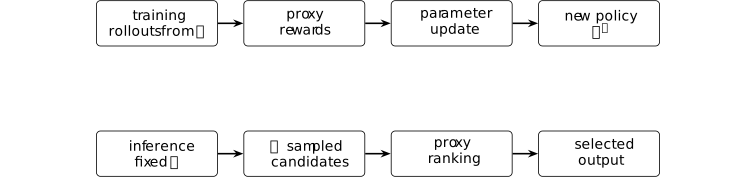
The lifecycle accounting of Definition [ftip-005H] places the first route's rollout and update work in separate coordinates. The second route incurs rollout and evaluation work but no parameter update. Consequently, the event $\mathcal E_N^{\rm fa}$ in Definition 2.5 concerns the candidate set presented to selection; it is not a claim about the selected output or a training-time policy change.

Remark 2.9. What verifier error rates do not identify [ftip-007O]

The rates in Definition [ftip-005Z] are properties of a declared audit law. They do not identify where errors occur within the task family, how error events depend across repeated candidates, or which accepted candidate a selector returns. Theorem 2.6 adds identical marginals and independence; Theorem 2.7 retains only the union bound.

Nor do these rates determine the effect of optimizing against the verifier. That effect depends on how the induced policy or selection law moves mass toward particular outcomes. The incomplete-checker example Example [ftip-0060] demonstrates one such movement, while Example 2.4 shows why an average reference-law error cannot rule it out. These are local finite statements. Any claim about a named verifier still requires its own audit distribution, evidence, and transfer argument.

The deterministic regret lemma Theorem 2.2, the independent-audit identity Theorem 2.6, and the union bound Theorem 2.7 follow from uniform approximation, independent trials, and subadditivity, respectively. Their hypotheses need not hold for a verifier chosen only for its empirical performance.

3. Feedback identifiability and fixed records [ftip-007P]

A training protocol can respond only to distinctions present in its observations. The following finite setup makes that restriction precise before considering stronger, model-specific limits on preference data.

Definition 3.1. Finite declared feedback protocol [ftip-007Q]

Fix a horizon $N\geq 0$, finite action sets $\mathcal A_n$, finite feedback sets $\mathcal F_n$, and a finite internal-seed set $\mathcal U$ with a declared law $\lambda $. A finite declared protocol $\mathsf P$ consists of selection maps

\[ a_n:\mathcal U\times \prod _{j<n}(\mathcal A_j\times \mathcal F_j) \longrightarrow \mathcal A_n \qquad (0\leq n<N). \]

An action may specify the task, rollout record, feedback request, or sampling choice made at that round. The protocol can depend on earlier exposed feedback and its declared seed, but it cannot depend on a latent world field that has not entered those arguments.

Definition 3.2. Finite feedback world [ftip-008C]

For the action and feedback sets of Definition 3.1, a finite feedback world $w$ supplies, for each round $0\leq n<N$, a probability kernel $K_{n,w}$ from a generic action--feedback history $(a_0,f_0,\ldots ,a_n)$ ending in $a_n\in \mathcal A_n$ to $\mathcal F_n$. Thus, whenever $a_j\in \mathcal A_j$ and $f_j\in \mathcal F_j$,

\[ K_{n,w}(\,\cdot \mid a_0,f_0,\ldots ,a_n) \in \Delta (\mathcal F_n). \]

Two worlds may agree on every feedback kernel queried by a protocol while differing in latent utility, unrequested labels, or unobserved environment facts. Those latent fields are not feedback until a declared query exposes them.

Definition 3.3. Observed feedback transcript [ftip-008D]

Fix a finite declared protocol $\mathsf P$ from Definition 3.1 and a finite feedback world $w$ from Definition 3.2. Draw $U\sim \lambda $ and, for $0\leq n<N$, set

\[ \begin {aligned} A_n&=a_n(U,A_0,F_0,\ldots ,A_{n-1},F_{n-1}),\\ F_n&\sim K_{n,w}(\,\cdot \mid A_0,F_0,\ldots ,A_n). \end {aligned} \]

The resulting observed feedback transcript is

\[ T_w^{\mathsf P}=(U,A_0,F_0,\ldots ,A_{N-1},F_{N-1}). \]

All protocol randomness is included in $U$. Immutable rollout records and typed feedback events may be components of the finite action and feedback sets, as in Definition [ftip-0051] and Definition [ftip-0053].

Definition 3.4. Observational equivalence for a declared protocol [ftip-007R]

Let $\mathcal T_{\mathsf P}$ be the finite set of possible transcripts for a declared protocol $\mathsf P$. Two feedback worlds $w_0,w_1$ are observationally equivalent for $\mathsf P$, written $w_0\equiv _{\mathsf P}w_1$, when

\[ \Pr (T_{w_0}^{\mathsf P}=t)=\Pr (T_{w_1}^{\mathsf P}=t) \qquad \text {for every }t\in \mathcal T_{\mathsf P}. \]

The relation is protocol-relative. Another protocol may issue a different feedback request and thereby separate the same worlds. Equality only on the realized transcript is weaker than this definition, which compares the whole finite transcript law.

Theorem 3.5. Post-training cannot distinguish observationally equivalent worlds [ftip-007S]

For a finite random variable $X$, write $\operatorname {Law}(X)$ for its probability law. If $h$ maps the value space of $X$ to a finite set $\mathcal Y$, its pushforward law $h_{\#}\operatorname {Law}(X)$ is characterized by \[ \bigl (h_{\#}\operatorname {Law}(X)\bigr )(\{y\}) =\Pr (h(X)=y),\qquad y\in \mathcal Y. \]

Let $w_0\equiv _{\mathsf P}w_1$. For any finite output set $\mathcal Y$ and any readout $h:\mathcal T_{\mathsf P}\to \mathcal Y$,

\[ h_{\#}\operatorname {Law}(T_{w_0}^{\mathsf P}) =h_{\#}\operatorname {Law}(T_{w_1}^{\mathsf P}). \]

Thus a final artifact stamp, update decision, or test chosen solely from the declared protocol's transcript has the same distribution in both worlds.

Proof.

For every $y\in \mathcal Y$, finiteness gives

\[ \begin {aligned} \Pr \left (h(T_{w_0}^{\mathsf P})=y\right ) &=\sum _{\substack {t\in \mathcal T_{\mathsf P}\\h(t)=y}} \Pr (T_{w_0}^{\mathsf P}=t)\\ &=\sum _{\substack {t\in \mathcal T_{\mathsf P}\\h(t)=y}} \Pr (T_{w_1}^{\mathsf P}=t) =\Pr \left (h(T_{w_1}^{\mathsf P})=y\right ). \end {aligned} \]

The middle equality is observational equivalence from Definition 3.4. These point probabilities determine the two pushforward laws.

This finite statement follows from the displayed hypotheses.

Remark 3.6. A no-free-feedback result, not a no-learning result [ftip-007T]

Theorem 3.5 says that the declared observations supply no information that distinguishes $w_0$ from $w_1$. It does not say that the output must equal the initial model, that the parameters cannot change, or that performance cannot improve in both worlds. Pretraining, inductive bias, computation on the observed records, and generalization may still produce an improvement shared by the two worlds.

Calling the theorem a no-learning result would therefore erase the central condition: only world-dependent conclusions unavailable from the common transcript are ruled out.

Corollary 3.7. Replaying a fixed pool supplies no new feedback information [ftip-007U]

Fix a realized finite replay pool $d$ as in Definition [ftip-0056]. Let $\mathcal V$ be a finite seed set, and let $V\in \mathcal V$ be a replay-and-update seed with the same declared law in two feedback worlds and whose law does not depend on the world. If a replay-only procedure makes no new environment or feedback query, then its output has the form $Y=h(d,V)$. The law of $Y$ is the same in the two worlds.

Proof.

For every output $y$,

\[ \Pr (h(d,V)=y)= \sum _{\substack {v\in \mathcal V\\h(d,v)=y}}\Pr (V=v). \]

The fixed pool, seed law, and readout are identical in the two worlds, so the displayed sum is identical. Equivalently, this is the pushforward argument of Theorem 3.5 applied after conditioning on the realized pool.

This finite statement follows from the displayed hypotheses.

Remark 3.8. Reuse can change optimization without enlarging evidence [ftip-007V]

A replay schedule can reweight records, reduce optimization error on the fixed pool, or produce a different update proposal in the sense of Definition [ftip-006C]. Those are genuine computational effects. They do not add a label, preference, verifier result, or environment transition to the fixed evidence. Fresh optimizer randomness is likewise not feedback about the latent world.

This distinction prevents sample reuse from being counted as feedback acquisition. It does not imply that replay is useless; it isolates the source of any benefit as further computation on already acquired records.

Example 3.9. Counterexample: An off-query utility reversal [ftip-007W]

Let the response set be $\{a,b\}$. A one-round protocol queries only $x_0$; both worlds return the preference $a\succ b$. The protocol therefore has the same transcript law in both worlds. Fix a deterministic transcript-to-policy readout that chooses $a$ also at an unqueried $x_1$. The worlds agree on every observed field but reverse utility at $x_1$:

$\text{[math]}$

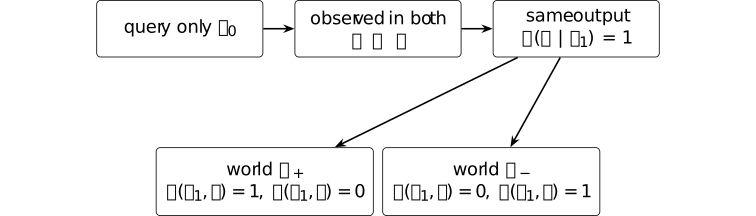
The transcript laws are identical, so Theorem 3.5 applies, while the deterministic readout returns the same output in both worlds. That output is optimal in $w_+$ and suboptimal in $w_-$ on $x_1$. The example does not show that generalization always fails. It shows that a claim about unqueried utility requires an assumption connecting observed feedback to that utility.

Remark 3.10. From finite indistinguishability to preference-data limits [ftip-007X]

[zhao2025limits, Theorems 3.3--3.5] study a more structured post-training model. They give ordinal-preference distortion lower bounds, including a lower bound under Bradley--Terry noise with linear scores, and a positive result using a limited number of cardinal queries. These results depend on the routing model, utility class, and query budget developed in § [ftip-008X].

Theorem 3.5 gives a finite pushforward theorem, while Example 3.9 gives a counterexample to identification from an incomplete transcript. They are neither proofs nor special cases of the paper's distortion results.

4. Replay monitors and trajectory compression [ftip-007Y]

Reusing a rollout and jumping along a predicted checkpoint path save different kinds of work. The first changes how often recorded feedback enters an update. The second replaces some realized training steps by a parameter forecast. This subsection records what their proposed monitors establish and, separately, what remains unmeasured.

Theorem 4.1. DGG head gradient and shared-weight occurrence sum [ftip-007Z]

Fix a sampled history and an active token $i$ in the interior of the unclipped branch of the GRPO objective. Consider a finite directed acyclic computation graph that is differentiable at the parameter point in question. Let $a_i$ be the sampled token, $\widehat A_i$ its fixed normalized advantage, and $p_i=\operatorname {softmax}(z_i)$ the current distribution on a finite vocabulary $\mathcal V$. With fixed behavior probability $b_i>0$, set \[ r_i=\frac {p_i(a_i)}{b_i}, \qquad \mathcal L_i=r_i\widehat A_i, \qquad E_i=r_i\widehat A_i(e_{a_i}-p_i). \] Here $e_{a_i}\in \mathbb R^{|\mathcal V|}$ is the sampled-token basis vector. The history and sampling decisions are held fixed during differentiation.

Suppose the output head $W_{\rm lm}\in \mathbb R^{|\mathcal V|\times d_{\rm model}}$ is untied: its only path to $\mathcal L_i$ is through $z_i=W_{\rm lm}h_{L,i}$, and $h_{L,i}\in \mathbb R^{d_{\rm model}}$ is independent of $W_{\rm lm}$. Then \[ G_i^{\rm lm}=\nabla _{W_{\rm lm}}\mathcal L_i =E_i h_{L,i}^{\mathsf T}. \]

Let $W_{\rm int}\in \mathbb R^{m\times d}$ be a shared intermediate weight. Index by a finite set $\mathcal O_i$ every occurrence of this weight that can affect $z_i$, assuming that all such uses have the form $y_o=W_{\rm int}x_o$, with $x_o\in \mathbb R^d$. First replace these uses by independent copies $W_o$ and evaluate them all at $W_o=W_{\rm int}$. Let $J_{io}\in \mathbb R^{|\mathcal V|\times m}$ be the downstream Jacobian from node $y_o$ to $z_i$ in this graph, with the other weight copies fixed. Define the contribution of occurrence $o$ by \[ H_{io}=\nabla _{W_o}\mathcal L_i =(J_{io}^{\mathsf T}E_i)x_o^{\mathsf T}. \] On tying the copies, the total derivative is \[ G_i^{\rm int}=\nabla _{W_{\rm int}}\mathcal L_i =\sum _{o\in \mathcal O_i}H_{io}. \] The head gradient and each occurrence contribution have rank at most one; the total shared-weight gradient need not.

For a layer used once per position in a causal network, the sum includes every earlier position whose output affects token $i$. Reuse across depth adds further occurrences. Tying the head to embeddings or other blocks also requires their contributions; the displayed head identity assumes that such tying is absent.

Proof.

Softmax differentiation gives $\nabla _{z_i}\mathcal L_i=E_i$. The outer-product rule gives the untied head identity. In the graph with independent copies, $x_o$ does not depend on its own $W_o$; all downstream paths from $y_o$ are included in $J_{io}$. The chain rule therefore gives $\nabla _{W_o}\mathcal L_i=(J_{io}^{\mathsf T}E_i)x_o^{\mathsf T}$. Finally, the derivative of the diagonal map $W_{\rm int}\mapsto (W_o=W_{\rm int})_{o\in \mathcal O_i}$ adds these partial derivatives.

Clipped or inactive terms require their own derivative or mask. [miao2026when, Section 4.2.1, Proposition 1, and Appendix A.1] derives the intermediate outer product through one local application. For a shared weight, that calculation gives $H_{io}$; identifying it with the total $G_i^{\rm int}$ omits the other occurrences. The sum above supplies the chain rule needed for shared parameters.

Theorem 4.2. DGG occurrence-to-head gradient-energy bound [ftip-0080]

Use the per-token quantities and untied head of Theorem 4.1, and fix one occurrence $o\in \mathcal O_i$. Assume $d_{\rm model}\geq 1$ and positive constants $\alpha _{\min }$, $\beta _{\max }$, and $C$ satisfy \[ \|h_{L,i}\|_2^2\geq \alpha _{\min }d_{\rm model}, \qquad \|x_o\|_2^2\leq \beta _{\max }d_{\rm model}, \] and the two logit-sensitivity bounds \[ \mathbb E_{a\sim p_i} \|(J_{io})_{a,:}\|_2^2\leq C, \qquad \|(J_{io})_{a_i,:}\|_2^2\leq C. \] If $\widehat A_i\neq 0$ and $p_i(a_i)<1$, then \[ \frac {\|H_{io}\|_F^2}{\|G_i^{\rm lm}\|_F^2} \leq \frac {\mathcal C_{\rm occ}} {(1-p_i(a_i))^2}, \qquad \mathcal C_{\rm occ} =\frac {4\beta _{\max }C}{\alpha _{\min }}. \]

Proof.

The sampled-token coordinate of $E_i$ and the lower activation bound give \[ \|G_i^{\rm lm}\|_F^2 =\|E_i\|_2^2\|h_{L,i}\|_2^2 \geq r_i^2\widehat A_i^2 (1-p_i(a_i))^2 \alpha _{\min }d_{\rm model}. \] Write $J_{io}^{\mathsf T}E_i$ as $r_i\widehat A_i$ times the difference between the sampled row and the $p_i$-weighted mean row. The squared-norm inequality $\|u-v\|_2^2\leq 2\|u\|_2^2+2\|v\|_2^2$, Jensen's inequality for that mean, and the two row-energy bounds give $\|J_{io}^{\mathsf T}E_i\|_2^2\leq 4r_i^2\widehat A_i^2C$. Hence \[ \|H_{io}\|_F^2 \leq 4r_i^2\widehat A_i^2C\, \beta _{\max }d_{\rm model}. \] The source's softmax probabilities make $r_i>0$; the nonzero-advantage and nonunit-probability hypotheses make the head lower bound positive. Division and cancellation give the displayed ratio.

This bounds one occurrence contribution, not the total derivative of a shared intermediate weight. For the latter, the sum in Theorem 4.1 gives only \[ \|G_i^{\rm int}\|_F \leq \sum _{o\in \mathcal O_i} \|J_{io}^{\mathsf T}E_i\|_2\|x_o\|_2. \] If the same displayed hypotheses hold for every occurrence, the triangle inequality yields the ratio bound $|\mathcal O_i|^2\mathcal C_{\rm occ}/(1-p_i(a_i))^2$ for $\|G_i^{\rm int}\|_F^2/\|G_i^{\rm lm}\|_F^2$. Controlling only the application at position $i$ does not establish this all-occurrence hypothesis or the source's claimed bound for the total gradient. The contributing positions, reuse pattern, and Jacobians depend on the architecture. Neither bound establishes a small gradient or an evaluation-score comparison.

The activation and row-energy hypotheses and the local inequality follow the calculation in [miao2026when, Section 4.2.1, Lemma 1, Assumption 1, Theorem 1, and Appendix A.3], with the differentiated object restricted to an occurrence contribution. They do not prove the source's total shared-weight claim under its local hypotheses.

Theorem 4.3. DGG finite-batch head-gradient inequality [ftip-0081]

For $T\geq 1$ active, unclipped tokens with fixed sampled histories and the untied output head of Theorem 4.1, let \[ G^{\rm lm}=\frac 1T\sum _{i=1}^T G_i^{\rm lm}, \qquad \overline {r^2}=\frac 1T\sum _{i=1}^T r_i^2, \] and set \[ c_{\max }= \max _{1\leq i\leq T} \widehat A_i^2 \|e_{a_i}-\pi _\theta (\mathord \cdot \mid h_{L,i})\|_2^2 \|h_{L,i}\|_2^2. \] Then \[ \|G^{\rm lm}\|_F^2\leq c_{\max }\overline {r^2} =c_{\max }(1+\widehat \chi ^2), \] where $\widehat \chi ^2$ is the statistic of Definition [ftip-0066]. If $c_{\max }>0$, rearrangement gives the source's equivalent direction \[ \widehat \chi ^2\geq \frac {\|G^{\rm lm}\|_F^2}{c_{\max }}-1. \]

Proof.

Convexity of the squared Frobenius norm and the factorization in Theorem 4.1 give \[ \left \|\frac 1T\sum _iG_i^{\rm lm}\right \|_F^2 \leq \frac 1T\sum _i\|G_i^{\rm lm}\|_F^2 \leq \frac {c_{\max }}T\sum _i r_i^2. \] The identity $\overline {r^2}=1+\widehat \chi ^2$ follows directly from Definition [ftip-0066]; division by positive $c_{\max }$ gives the final form.

The inequality points from observed head-gradient energy to a lower bound on this finite-batch squared-ratio statistic. It is not a converse: cancellation can hide nonunit ratios. The active cancellation example in Example 4.6 states its clipping interval explicitly. The proof uses no intermediate-weight bound.

The finite-batch inequality follows the calculation in [miao2026when, Section 4.2.2, Lemma 2, Theorem 2, and Appendix B], under the untied-head and fixed-history assumptions stated above.

Remark 4.4. DGG monitors update geometry, not evaluation safety [ftip-0082]

The identities in Theorem 4.1--Theorem 4.3 concern gradients, importance ratios, activations, and occurrence-specific logit Jacobians. The intermediate bound controls a local contribution; a shared-weight bound needs control over all contributing occurrences. None of their hypotheses mentions the fixed independent-evaluation functional $J_{\rm ev}$ of Definition [ftip-005E]. They therefore cannot imply that accepting an update preserves $J_{\rm ev}$, or that rejecting one would have prevented a decrease.

DGG adds an empirical policy on top of those identities: it monitors the increment in head-gradient energy, standardizes that increment against a trailing window, and rejects some reused updates before the optimizer step [miao2026when, Section 5 and Algorithm 1]. Its reported experiments relate that policy to observed training stability. They do not turn the Z-score into a calibrated test of independent-evaluation safety.

Example 4.5. Counterexample: empirical squared-ratio excess can be negative [ftip-0083]

Take one observed action $a$ with $\pi _{\rm old}(a)=1/2$ and $\pi _\theta (a)=1/4$. The batch contains only that action, so $T=1$ and $r_1=1/2$. Hence \[ \widehat \chi ^2=r_1^2-1=-\frac 34. \] Both policies can be completed on a two-action space by assigning their remaining mass to the other action.

Thus the finite-batch statistic in Definition [ftip-0066] need not share the nonnegativity of the population Pearson divergence. Theorem Theorem 4.3 remains valid: its right side contains $1+\widehat \chi ^2=1/4=\overline {r^2}$.

Example 4.6. Counterexample: active batch cancellation can hide nonunit ratios [ftip-0084]

Fix $\epsilon _{\rm clip}\in (0,1)$ and $1<R<1+\epsilon _{\rm clip}$. On a two-token vocabulary, let both observed tokens have $a_i=1$, current probability $\pi _\theta (1)=1/2$, and behavior probability $\pi _{\rm old}(1)=1/(2R)$. Take scalar hidden states $h_{L,1}=h_{L,2}=1$ and fixed normalized advantages $\widehat A_1=1$, $\widehat A_2=-1$. These may be selected token terms from different rollout members. An untied head with both logits zero realizes the current probabilities. Both terms lie strictly inside the clipping interval of Definition [ftip-003F], so the clipped surrogate locally agrees with $\mathcal L_i=r_i\widehat A_i$. Thus $r_1=r_2=R$, and Theorem 4.1 gives \[ G_1^{\rm lm}=R(1/2,-1/2)^{\mathsf T}, \qquad G_2^{\rm lm}=-G_1^{\rm lm}. \] Consequently $G^{\rm lm}=0$, while $\widehat \chi ^2=R^2-1>0$. For this fixed clipping rule, the statistic in this construction is bounded above by $(1+\epsilon _{\rm clip})^2-1$.

For the raw surrogate $\mathcal L_i=r_i\widehat A_i$ considered as a separate objective, the same algebra works at every $R>1$ and yields arbitrarily large squared-ratio excess. This does not extend the active construction to arbitrary $R$ under clipping: when $R>1+\epsilon _{\rm clip}$, the positive-advantage term is locally constant, while the negative term remains active. Their clipped gradients are then $0$ and $-R(1/2,-1/2)^{\mathsf T}$, with nonzero mean $(-R/4,R/4)^{\mathsf T}$.

The example does not contradict Theorem 4.3: that theorem upper-bounds batch-gradient energy by a ratio moment. It supplies no lower bound on the gradient and no converse from zero batch-gradient energy to ratios equal to one. The arbitrary-ratio version concerns only the separate raw surrogate.

Example 4.7. Counterexample: a Z-score gate is not an evaluation-safety certificate [ftip-0085]

Let two consecutive proposed reused updates have the same monitored energy, $g_{t-1}=g_t=1$. With trailing-window increment mean $\mu _t=0$, any positive scale $\sigma _t+\varepsilon $, and any positive threshold, DGG's score is \[ z_t=\frac {(g_t-g_{t-1})-\mu _t}{\sigma _t+\varepsilon }=0, \] so the gate accepts the proposal. Now choose a fixed evaluation interface for which the artifact before the accepted update has performance $J_{\rm ev}=1$ and the artifact after it has performance $J_{\rm ev}=0$.

This is consistent because the gate rule of Definition [ftip-005A] imposes no mathematical relation between its scalar monitor and $J_{\rm ev}$. A safety claim would need an additional assumption connecting proposed updates to the independent evaluation law; the Z-score calculation alone cannot provide it.

Definition 4.8. Leading squared singular-energy share [ftip-0086]

Let $\Delta W\in \mathbb R^{m\times n}$ be nonzero, set $q=\min (m,n)$, and order its singular values as $\sigma _1\geq \cdots \geq \sigma _q\geq 0$. Its leading squared singular-energy share is \[ \rho _1(\Delta W) =\frac {\sigma _1(\Delta W)^2}{\sum _{j=1}^q\sigma _j(\Delta W)^2} =\frac {\sigma _1(\Delta W)^2}{\|\Delta W\|_F^2}. \] The nonzero hypothesis prevents an undefined $0/0$; the value lies in $[1/q,1]$.

NExt instead reports $E_1=\sigma _1/\sum _j\sigma _j$ in Section 3.2 Low-rank optimization trajectories modeling for LLM RLVR acceleration[chen2026lowrank]. That nuclear-share statistic and $\rho _1$ answer different questions. The squared share measures contribution to squared Frobenius norm.

Definition 4.9. Leading spectral gap [ftip-0087]

For $\Delta W\in \mathbb R^{m\times n}$ with $q=\min (m,n)\geq 2$, its leading spectral gap is \[ \operatorname {gap}_1(\Delta W) =\sigma _1(\Delta W)-\sigma _2(\Delta W). \] A positive gap makes the leading left and right one-dimensional singular subspaces unique, although each chosen singular vector still has an arbitrary sign. When the gap is zero, a single leading vector is not intrinsic.

The quantity is undefined when $q=1$, since there is no second singular value. Projector comparisons require a positive gap at every compared checkpoint.

Definition 4.10. Leading-subspace projector drift [ftip-0088]

Let $\Delta W_t$ and $\Delta W_s$ be nonzero matrices of the same shape, each with positive leading spectral gap. If $u_1(t)$ and $u_1(s)$ are unit leading left singular vectors, define their leading-subspace projector drift by \[ d_{\rm proj}(t,s) =\|\Pi _t^{\rm svd}-\Pi _s^{\rm svd}\|_F, \qquad \Pi _t^{\rm svd}=u_1(t)u_1(t)^{\mathsf T}, \quad \Pi _s^{\rm svd}=u_1(s)u_1(s)^{\mathsf T}. \] The definition is independent of both singular-vector signs and takes values in $[0,\sqrt {2}]$.

This is an additional proposed trajectory diagnostic; NExt does not define it.

A large value of $\rho _1$ from Definition 4.8 says that one singular mode dominates a particular difference matrix. It does not say that the dominant subspace remains fixed across checkpoints; $d_{\rm proj}$ measures that separate question.

Definition 4.11. Path-emulation regret [ftip-0089]

Fix the evaluation interface of Convention [ftip-005D]. Let $P_{t+s}^{\rm act}$ be the protocol that returns the artifact reached after $s\geq 1$ additional realized training steps from checkpoint $t$. Let $\mathcal K_{\leq t}$ be the saved checkpoint history available through $t$, and let $\widehat P_{t+s}(\mathcal K_{\leq t})$ instead return the artifact forecast from that history. Their signed path-emulation regret and absolute path-emulation regret are \[ \begin {aligned} \operatorname {Reg}^{\rm path}_{\rm ev}(t,s) &=J_{\rm ev}(P_{t+s}^{\rm act}) -J_{\rm ev}(\widehat P_{t+s}(\mathcal K_{\leq t})),\\ \operatorname {AReg}^{\rm path}_{\rm ev}(t,s) &=\left |\operatorname {Reg}^{\rm path}_{\rm ev}(t,s)\right |. \end {aligned} \]

The sign distinguishes an optimistic forecast from a pessimistic one; the absolute value measures discrepancy without cancellation across checkpoints. Both use the same task law, inference budget, and evaluator. Parameter error alone is not substituted for evaluation error. The NExt extrapolation and recovery schedule described in Sections 4.1--4.3 and 5.1 motivates this comparison Low-rank optimization trajectories modeling for LLM RLVR acceleration[chen2026lowrank], but the paper does not state this regret definition.

Example 4.12. Counterexample: early low-rank agreement does not determine continuation [ftip-008A]

Let $e_1=(1,0)^{\mathsf T}$ and $e_2=(0,1)^{\mathsf T}$ be the standard basis vectors of $\mathbb R^2$. In a two-dimensional matrix chart, set $P=e_1e_1^{\mathsf T}$ and $Q=e_2e_2^{\mathsf T}$. Two paths share the entire observed history \[ W_0=0,\qquad W_1=P,\qquad W_2=2P. \] Every observed local difference is the same rank-one matrix $P$. The paths then fork: path A takes $W_3^A=3P$, whereas path B takes $W_3^B=2P+Q$. Each next local difference is again rank one.

$\text{[math]}$

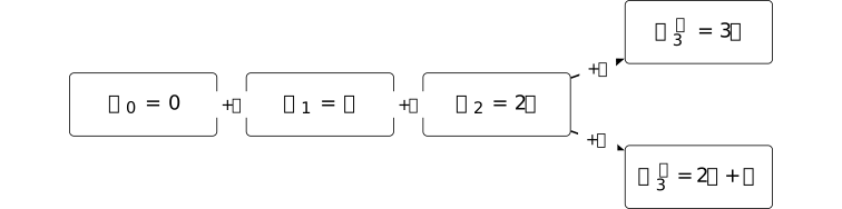
A deterministic history-only forecaster must return the same matrix $\widehat W_3$ in both worlds. Since $\|W_3^A-W_3^B\|_F=\|P-Q\|_F=\sqrt {2}$, the triangle inequality forces its Frobenius error to be at least $1/\sqrt {2}$ on one continuation. Low-rank early motion therefore does not identify the next subspace or the next checkpoint.

Remark 4.13. Compression of a charted path is not capability acquisition [ftip-008B]

NExt extracts global, local, and target differences from LoRA checkpoint matrices, keeps leading singular factors, learns a nonlinear predictor, jumps in that parameter chart, and resumes RLVR [chen2026lowrank, Sections 3.2, 4.1--4.3, and 5.1]. Its reported results are empirical; the paper states no theorem that a leading subspace remains stable or that a forecast preserves a policy.

The quantities in Definition 4.8--Definition 4.11 separate four tests. Squared singular-energy share concerns one matrix, spectral gap controls whether its leading subspace is identifiable, projector drift compares those subspaces over time, and path-emulation regret returns to fixed independent evaluation. None, by itself, is evidence that new feedback was acquired or that a new capability was learned. Such a claim must use a declared post-training gain such as Definition [ftip-005F] and must charge forecast training, the parameter jump, and recovery updates.