Given the base artifact \(M_0=(\tau ,\delta ,\mathsf {cfg},\theta _K,\mathsf {num})\) from Definition [ftip-001K], a fine-tuning run declares training records, a finite update count \(J\geq 0\), a loss \(L_{\rm ft}\), gradient estimators \(g_j^{\rm ft}\), optimizer states \(s_j^{\rm ft}\), and update specifications \((U_j,\eta _j^{\rm ft})\). It starts from \(\theta ^{\rm ft}_0=\theta _K\).

For each \(j=0,\ldots ,J-1\), the update is

Its output artifact replaces \(\theta _K\) by the final \(\theta ^{\rm ft}_J\). Any change to the tokenizer, architecture configuration, numerical convention, or other artifact field must be stated separately. Fine-tuning is not identified with one loss or data type.

In the cited pipeline, supervised fine-tuning (SFT) starts from a pretrained GPT-3 checkpoint and updates it by supervised learning on labeler demonstrations. The resulting policy supplies the starting and reference policy for later stages.

Appendix C.1 reports optimization choices for that construction. It does not define a universal mask, weighting rule, or fine-tuning protocol.

Wei et al. train on instruction-expressed task mixtures in [wei2022finetuned, Section 2 and Figure 2]. Ouyang et al. fine-tune on labeler demonstrations in [ouyang2022training, Section 3.5 and Appendix C.1]. The proposed continued-optimization interface in Definition 1.1 includes these concrete supervised instances.

Neither cited source defines fine-tuning as one universal objective. A concrete run must state its records, loss and normalization, optimizer, stopping rule, and trainable parameters. Instruction tuning later specializes the records to instruction--response demonstrations.

Let \(\mathcal X_{\mathrm {pr}}\) be the prompt space. For each prompt \(x\in \mathcal X_{\mathrm {pr}}\), let \(\mathcal Y(x)\subseteq \mathcal V^*\) be the set of finite token responses permitted by the training format. We write \(y=(y_1,\ldots ,y_{|y|})\in \mathcal Y(x)\) and \(y_{<t}=(y_1,\ldots ,y_{t-1})\).

A demonstration is denoted \(z=(x,y,\omega )\), where \(\omega \) is its provenance record. A finite multiset of demonstrations is denoted \(D_{\mathrm {sft}}\). For each response position, a loss mask \(m_t(z)\in \{0,1\}\) records whether the token contributes to the supervised objective, and a nonnegative weight \(w_t(z)\) records its declared normalization. Prompt tokens are conditioning context and lie outside the response-position domains of \(m_t(z)\) and \(w_t(z)\).

Using the prompt space of Notation 2.1, a prompt serializer is a declared map \[ s_{\mathrm {pr}}:\mathcal X_{\mathrm {pr}}\longrightarrow \mathcal V^*. \] For token strings \(u,v\in \mathcal V^*\), write \(u\mathbin {\Vert }v\) for their concatenation. A response token \(y_t\) is therefore predicted from the token prefix \(s_{\mathrm {pr}}(x)\mathbin {\Vert }y_{<t}\).

The serializer fixes system text, role markers, separators, and any other prompt-side control tokens. Changing it changes the conditional examples seen by the language model even when the abstract prompts and responses are unchanged.

The next-token law in Definition [ftip-000H] accepts token prefixes, whereas an instruction dataset may store structured prompts. The proposed serializer in Definition 2.2 maps between those types. Ouyang et al. describe SFT on labeler demonstrations in [ouyang2022training, Section 3.5 and Appendix C.1]; their training account supplies a concrete pipeline rather than a universal serializer.

A reproducible objective must retain the serializer revision with the tokenizer and loss mask. Otherwise two runs can share an abstract dataset name while optimizing different token sequences.

Instruction tuning fine-tunes a pretrained language model on a mixture of tasks whose examples are expressed through natural-language instructions and corresponding target outputs. The task description and any input are placed in the prompt; the target output supplies the continuation to be learned.

The construction changes the model parameters by supervised learning. It does not require a learned reward model, preference comparisons, or interaction with an environment.

Using the notation of Notation 2.1, a demonstration record is a triple

where \(\omega \) identifies the declared producer of \(y\), the collection or generation procedure, and any selection rule applied before the record entered \(D_{\mathrm {sft}}\). The response is a training target; its presence in the data does not assert that it is uniquely correct or preferred to every alternative.

The provenance field \(\omega \) distinguishes a demonstration from the process that supplied it. Ouyang et al. collect labeler-written demonstrations in [ouyang2022training, §§3.2, 3.4]. Wei et al. permit a broader task mixture in [wei2022finetuned, §2; Fig. 2].

Human writers, stronger teacher models, filtered self-generations, and programmatically produced targets give different information to the learner. Claims about sample efficiency or capability acquisition must therefore state which producer and selection rule were available.

In the InstructGPT data-collection procedure, a labeler receives a prompt and writes a desired response. The resulting prompt--response pair enters the demonstration data used by the supervised fine-tuning stage. Prompts come from the declared API and labeler-written sources, and the paper records filtering and labeler-selection procedures.

This construction specifies a human demonstration channel. It is distinct from the later comparison channel, in which a labeler ranks model-generated responses rather than writing the target response.

For the language-model policy \(\pi _\theta \) and the notation of Notation 2.1, a masked supervised fine-tuning (SFT) objective has the form

where the nonnegative weights satisfy \(\sum _{z\in D_{\mathrm {sft}}}\sum _{t=1}^{|y|}w_t(z)m_t(z)=1\). The response index \(t\) does not range over serialized prompt tokens. Minimizing this objective increases conditional likelihood on the selected target tokens. The weights and mask are local conventions and must be declared for each implementation.

For a finite demonstration multiset, define the number of selected response tokens by

When \(N_{\mathrm {resp}}>0\), response-token normalization sets \(w_t(z)=N_{\mathrm {resp}}^{-1}\) at every selected position. Each selected token then has equal weight in \(L_{\mathrm {sft}}\). Equal weighting of records or prompts is a different convention because response lengths vary.

The training account alone does not determine this normalization. Any comparison of losses or gradients must retain the mask and normalization that produced them.

Two instruction positions provide conditioning context but lie outside the response-loss index set. The loss is taken on the two generated tokens.

Declare \(\pi (r_1\mid u_1,u_2)=1/2\) and \(\pi (r_2\mid u_1,u_2,r_1)=1/4\). The instruction tokens are not indexed by the response mask. With mask one on each displayed response token, the sum and mean are \[ L_{\rm sum}=-\log \tfrac 12-\log \tfrac 14=\log 8, \qquad L_{\rm mean}=\tfrac 12\log 8\approx 1.040. \]

The supervised objective in Definition 2.8 and the causal factorization in Definition [ftip-000I] specialize to the displayed token strip. Its mask is a local choice on response positions; other instruction-tuning implementations may supervise a different subset of response tokens or declare a larger loss domain explicitly.

Instruction tuning changes conditional likelihood under a declared demonstration distribution. It can teach response format, task interpretation, and behavior represented by the targets, but the training loss alone does not identify which of those effects caused an independent evaluation gain.

Ouyang et al. report supervised fine-tuning and its optimization settings in [ouyang2022training, Section 3.5 and Appendix C.1]. They do not define the exact mask and weighting convention displayed in Definition 2.8; those choices remain part of the declared objective.

The stage also leaves several questions open. A demonstration does not compare its target with alternatives, a teacher may transmit errors or hidden information, and low loss on the collected prompts need not imply transfer to a new task law. Preference acquisition introduces a different observation: which response a judge selected from a displayed pair.

Use the prompt and response spaces from Notation 2.1. A comparison query is a displayed triple \(c=(x,y^0,y^1)\) with \(y^0,y^1\in \mathcal Y(x)\). Let \(\mathcal J\) be the declared judge population, and let \(j\in \mathcal J\) identify the human, model, or rule that returns a comparison label \(b_{\mathrm {pref}}\in \{0,1\}\).

When \(b_{\mathrm {pref}}=1\), write \(y^+=y^1\) and \(y^-=y^0\); when \(b_{\mathrm {pref}}=0\), reverse those names. Thus \(y^+\) means selected in this observation, not objectively or uniquely best. The acquisition mechanism may also record a tie, abstention, or invalid comparison, but those outcomes must use an enlarged label space rather than being silently forced into \(\{0,1\}\).

Restrict attention to a comparison for which the judge selects one displayed alternative rather than reporting indifference or incomparability. For a query \(c=(x,y^0,y^1)\) and a judge \(j\), a pairwise comparison observation is the displayed pair together with the judge's selected alternative. In winner--loser notation it is recorded as

The observation reports a choice made under the declared presentation and query procedure. It does not by itself provide a numerical reward, a complete ranking of responses, or a judgment about alternatives that were not shown.

Preference learning may choose which trajectory segments or responses to show to a judge rather than sampling every pair uniformly. The query-selection procedure assigns candidate comparisons a priority derived from the current reward-model ensemble and requests labels for selected pairs.

Because selection depends on the current model and candidate pool, the resulting comparison data reflect an acquisition policy. Active selection can concentrate labels on uncertain pairs, but it does not make the collected comparisons representative of an undeclared target population.

A preference observation depends on the query presented and the judge who evaluates it. Concrete elicitation procedures include [christiano2017deep, Sections 2.2.2 and 2.2.4] and the language-model comparison pipeline of [ouyang2022training, Sections 3.2 and 3.4].

The response generator, pair-selection rule, presentation order, judge population, and aggregation rule can each change the observed law. A later sample-complexity or population claim must condition on those choices rather than treating comparison labels as an unqualified source of ground truth.

A preference data law \(\mathcal D_{\mathrm {pref}}\) is a probability law on pairwise comparison observations \(o=(x,y^+,y^-,j)\) from Definition 3.2. It includes the randomness of prompt selection, response generation, pair selection, judge selection, and the judge's reported label.

A finite training multiset \(D_{\mathrm {pref}}=(o_1,\ldots ,o_N)\) is sampled or adaptively collected under that law and its acquisition history. When queries are adaptive, the records need not be independent or identically distributed.

A scalar reward model is a parameterized function

whose score is fitted from comparison observations. The score orders or weights responses for a specified training procedure; it is not automatically the independent utility of the response. Ouyang et al. initialize the model from the supervised policy and replace its language-model head with a scalar output for this stage.

Given scalar scores for two alternatives, the Bradley--Terry comparison law assigns the probability

where \(\sigma (a)=(1+\exp (-a))^{-1}\). Conditioning the scores on a language-model prompt is the contextual specialization used in modern reward modeling; see also [rafailov2023direct, Section 3, equation (1)].

For comparison observations sampled from \(\mathcal D_{\mathrm {pref}}\), the pairwise reward-model loss is

The empirical objective replaces the expectation by a declared weighting of the collected comparisons. It fits score differences under the Bradley--Terry law of Definition 3.7; it does not observe an absolute reward target for either response.

Fitting a Bradley--Terry predictor is an assumption about representation, not a consequence of observing comparisons. Cyclic choices, context effects, and mixtures of judges can fail to agree with one shared scalar ordering.

Even within the model, scores are not identified absolutely: replacing \(r_\phi (x,y)\) by \(r_\phi (x,y)+c(x)\) leaves every pairwise probability and the loss unchanged. Ouyang et al. give one normalization in [ouyang2022training, §3.5; App. C.2]. Other uses must state their own normalization, judge population, and validation law.

A declared difference between two reward scores maps to one Bradley--Terry preference probability.

Under the Bradley--Terry link, \[ \Pr (y^+\succ y^-\mid x) =\frac {\exp r(y^+)}{\exp r(y^+)+\exp r(y^-)} =\sigma (2-0.5) =\sigma (1.5)\approx 0.8176. \] Reversing the pair gives probability \(1-0.8176=0.1824\).

The fixed scores instantiate Definition 3.7 and determine the displayed probability. Whether one scalar reward can represent every judge is a separate modeling question.

A reward-model validation law \(\mathcal D_{\mathrm {rm}}^{\mathrm {val}}\) is a held-out law on comparison observations used to evaluate the fitted score model rather than to update \(\phi \). A declared validation statistic may be Bradley--Terry log loss or the probability that \(r_\phi (x,y^+)>r_\phi (x,y^-)\).

The validation population and acquisition procedure are part of the quantity. Accuracy on comparisons drawn from the same collection process does not establish calibration under a new judge population or agreement with an independent task-success criterion.

Ouyang et al. hold out comparison data and report reward-model validation accuracy and loss in [ouyang2022training, Section 3.5 and Appendix C.2]. Representing the validation population by a probability law makes the estimand depend explicitly on the judge population and acquisition procedure.

This law belongs to reward-model validation. It is not the independent task evaluation used later to compare post-training protocols.

Three strict comparisons arranged in a directed cycle obstruct representation by a single scalar ordering.

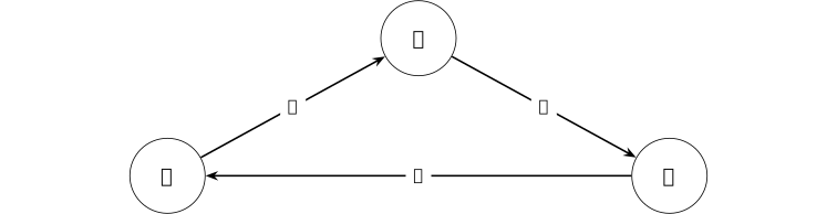
Declare \(A\succ B\), \(B\succ C\), and \(C\succ A\). If a scalar \(r\) represented all three comparisons by strict inequalities, then \[ r(A)>r(B)>r(C)>r(A), \] which implies \(r(A)>r(A)\), a contradiction. Thus no real-valued score can represent this cycle by ordinary greater-than.

Scalar pairwise reward modeling is used in [christiano2017deep, Section 2]; the finite cycle marks one assumption needed for that reduction. No empirical cycle is attributed to a particular dataset or population, and the obstruction concerns scalar orderings rather than all preference models.

The ratio and policy-objective formulas in this section specialize the measurable policy interface of Definition [ftip-0023] to a declared finite or countable discrete action space. Thus \(\pi (a\mid h)\) denotes probability mass, not an unspecified density. Whenever \(\log \pi _\theta (A_t\mid H_t)\) is displayed, its sampled mass is assumed positive.

For decision times \(t=0,\ldots ,N-1\), write \(\mathsf H_t:=H_t\) for the public history defined in Definition [ftip-0021], \(A_t\) for its action, and \(R_{t+1}\in \mathbb R\) for the next reward. Let \(\gamma \in [0,1]\) be the discount factor and \(G_t\) the return from time \(t\).

Write \(\pi _b\) for the behavior policy that produced a stored action, \(\pi _\theta \) for the current trainable policy, and \(\pi _{\mathrm {ref}}\) for a fixed reference policy. Their value, action-value, and advantage functions are denoted \(V^\pi \), \(Q^\pi \), and \(A^\pi \); an estimated advantage is \(\widehat A_t\). The current-to-behavior likelihood ratio is denoted \(\rho _t(\theta )\).

In a response-level episode, \(\pi _\theta (y\mid x)\) abbreviates the completed-continuation probability \(P_\theta (y\mid s_{\mathrm {pr}}(x))\) of the response-task interface, using the declared prompt serializer; the same convention applies to \(\pi _b\) and \(\pi _{\mathrm {ref}}\). In an interactive episode these symbols instead denote the action laws on public histories defined in Definition [ftip-0023].

In the response-level specialization used for language-model RLHF, a prompt \(x\) is the initial context, a complete response \(y\sim \pi _\theta (\mathord \cdot \mid x)\) is the sampled action, and a scalar score supplies the terminal reward. The episode terminates after that response.

This contextual-bandit view is sufficient for sequence-level reward-model training. Token generation may still be exposed as multiple policy decisions when an optimizer assigns token-level likelihood ratios or advantages. A later agentic setting also permits environment observations and tool actions between model responses.

A scalar reward \(R_{t+1}\in \mathbb R\) is the numerical signal received after action \(A_t\) and before the next decision. Its probabilistic law may depend on the current history, action, and environment transition.

Reward specifies the training objective of the reinforcement-learning problem. It need not equal an independent evaluator's utility, and a terminal reward need not identify which earlier action caused the outcome.

For an episode ending at time \(N\), the return from decision time \(t\) is

When all intermediate rewards vanish, every return is determined by the terminal reward, up to discounting. Return is a random variable under the policy and environment law; its expectation defines value.

For a policy \(\pi \), the value function and action-value function are

whenever the conditional expectations exist. Both quantities depend on the reward, transition law, horizon, discount, and the policy followed after the conditioned decision.

For a policy \(\pi \), its advantage function is

The advantage compares an action with the policy's average continuation value at the same information state. Policy-gradient implementations replace it by an estimator \(\widehat A_t\); the estimator and the mathematical advantage are not interchangeable without assumptions on bias and variance.

Subtracting a baseline that does not depend on the sampled action can reduce the variance of a policy-gradient estimator without changing its expected gradient under the source conditions. A learned value function, a group mean, and a leave-one-out mean are different baselines and have different finite-data dependencies.

An estimated advantage may use sampled returns, bootstrapped values, or a mixture of both. Its error enters the update even when the likelihood-ratio calculation is exact.

The behavior policy \(\pi _b\) is the policy that generated a sampled action. The current policy \(\pi _\theta \) is the policy whose parameters are being optimized. Proximal policy optimization (PPO) collects a batch under an old policy and then compares candidate current policies with that data.

A reference policy \(\pi _{\mathrm {ref}}\) is instead held fixed to define a regularizer or preference objective; see [rafailov2023direct, Section 3, equation (3)]. It need not equal the behavior policy that generated a later rollout.

For an action \(A_t\) sampled from \(\pi _b\) at information state \(\mathsf H_t\), the current-to-behavior likelihood ratio is

The ratio is defined on sampled actions for which \(\pi _b(A_t\mid \mathsf H_t)>0\). A bounded or clipped sampled ratio does not by itself control policy probabilities at unvisited histories.

For a nonempty finite index set \(I\) and real values \((Z_i)_{i\in I}\in \mathbb R^I\), write \[ \widehat {\mathbb E}_{i\in I}[Z_i] =\frac 1{|I|}\sum _{i\in I}Z_i. \] When the subscript is only \(t\), the index set is the declared collection of sampled decision times in the current batch.

PPO uses empirical expectation notation for its sampled surrogates; see Section 2, equations (1)--(2) of [schulman2017proximal]. The batch and its weighting must still be declared; the hat does not assert unbiasedness.

For samples collected under the declared behavior law and estimated advantages \(\widehat A_t\), the empirical policy-gradient surrogate is the following sample average:

Its gradient is the familiar score-function estimator. The sampled states, actions, and advantage estimator are held fixed while differentiating this surrogate; changing the data-collection law defines a different estimator.

On a three-step episode, a discounted return and a baseline-relative advantage can be computed separately.

Take discount \(\gamma =1/2\). The return attached to the first action is \[ G_0=r_1+\gamma r_2+\gamma ^2 r_3 =0+\tfrac 12+\tfrac 14\cdot 2=1. \] If the declared baseline is \(V(s_0)=0.4\), then the corresponding advantage estimate is \(\widehat A_0=G_0-V(s_0)=0.6\).

The calculation instantiates the return and advantage in Definition 4.4 and Definition 4.6. It illustrates one baseline choice. Low variance and correct attribution of terminal reward to an internal decision require additional assumptions or evidence.

A terminal response score can be copied into returns for many token decisions, but that bookkeeping does not reveal which token caused the score.

Monte Carlo returns, learned values, generalized advantage estimation, and group-relative normalization make different bias, variance, and dependence choices. Any theorem about an update must name the estimator actually used, the behavior policy that supplied its samples, and the horizon over which its credit signal is propagated.

An alignment-training claim is a capability claim \((M_0,A,E_{\rm align},b)\) in the sense of Convention [ftip-0003]. The procedure \(A\) changes model parameters and declares its training observations, loss or reward, and update rule. The independently fixed criterion \(E_{\rm align}\) states the behavior relative to which the word ``alignment'' is used.

Calling a procedure alignment training does not assert that its criterion is complete or that optimizing its training signal improves an independent evaluation.

Ouyang et al. combine demonstrations, comparison-trained rewards, and PPO in [ouyang2022training, Sections 3.1--3.5]. Direct Preference Optimization replaces the learned-reward PPO stage with a preference loss in [rafailov2023direct, Section 4]. The broader alignment-training description is a proposed way to compare such routes; it does not identify their observations or objectives with one another.

The declared behavioral criterion is part of the claim, while the independent evaluation remains a separate object. Their agreement is an empirical or theoretical claim, not a consequence of the word alignment.

The InstructGPT pipeline first performs supervised fine-tuning on labeler demonstrations. It then samples response pairs, collects labeler rankings, and fits a scalar reward model. Finally, it samples responses from the trainable policy and applies PPO using the reward-model score together with a penalty relative to the supervised policy.

The three stages consume different records and optimize different losses. Calling their composition RLHF does not make supervised targets, pairwise preferences, learned rewards, and policy-gradient samples the same kind of feedback.

The RLHF pipeline makes three logically separate choices. The comparison data specify which judgments were observed; the reward model specifies how those observations are represented and generalized; the policy optimizer specifies how sampled actions change the model.

An alignment criterion lies outside this chain unless it is identified with the training reward by assumption. A reward model can predict its held-out comparisons while failing under policy-induced distribution shift, and PPO can increase the learned reward while independent utility stays fixed or falls.

For probability mass functions \(p\) and \(q\) on a finite or countable set \(\mathcal Y\), the Kullback--Leibler divergence of \(p\) relative to \(q\) is \[ D_{\mathrm {KL}}(p\Vert q) =\sum _{y\in \mathcal Y}p(y)\log \frac {p(y)}{q(y)}. \] We use \(0\log (0/q)=0\). If \(p(y)>0\) and \(q(y)=0\) for some \(y\), the value is \(+\infty \). On a countable set, the negative part of the displayed series is finite; a divergent positive part gives the value \(+\infty \). Since \(\mathcal V^*\) is countable, the definition applies to the response laws of Notation 2.1.

The order of the arguments matters. In particular, finiteness of the displayed forward divergence requires \(p\) to be absolutely continuous with respect to \(q\).

The KL-regularized reward objective appears as equation (3) in Section 3 of [rafailov2023direct]. Behavior-policy ratios, clipped ratios, and KL penalties enter alignment objectives for different purposes.

A coefficient multiplying \(D_{\mathrm {KL}}\) declares an optimization tradeoff. It is neither a guarantee that every sampled ratio is small nor an independent evaluation of the resulting policy.

Let \(\mu \) be a prompt law, \(r(x,y)\) a scalar reward, and \(\pi _{\mathrm {ref}}\) a fixed reference policy. For \(\beta >0\), the KL-regularized RLHF objective, using forward KL, is

The prompt law, reward, reference policy, and coefficient are part of the objective. The forward KL requires the optimized policy to be absolutely continuous with respect to the reference wherever the objective is finite.

For a prompt \(x\), sampled response \(y\), learned reward score \(r_\phi (x,y)\), and fixed reference policy \(\pi _{\mathrm {ref}}\), the sequence-level KL-shaped reward is

Autoregressive factorization writes the logarithmic term as a sum of token-level log ratios. Ouyang et al. also mix a pretraining-gradient term into their reported PPO objective; that auxiliary term is separate from the shaped reward displayed here.

Given an approximate value function \(V\), with \(V(\mathsf H_N)=0\) at a terminal information state, define the temporal-difference residual

For \(\lambda \in [0,1]\), the finite-episode generalized advantage estimator is

The parameters \(\gamma \) and \(\lambda \) trade temporal reach against the variance and approximation error induced by bootstrapping. The estimator also depends on the fitted value function.

For a clipping parameter \(\epsilon _{\mathrm {clip}}\in (0,1)\), define \(\operatorname {clip}_{\epsilon _{\mathrm {clip}}}(u) =\min (1+\epsilon _{\mathrm {clip}},\max (1-\epsilon _{\mathrm {clip}},u))\). The PPO clipped surrogate is

Clipping changes the sampled surrogate when the ratio moves outside the declared interval in a direction favored by the estimated advantage. It is not a hard bound on the KL divergence of the complete updated policy.

PPO implementations may optimize the combined sampled objective

Here \(L_t^{\mathrm {CLIP}}\) is the per-sample integrand of the clipped surrogate in Definition 6.8, \(c_1,c_2\geq 0\), \(\widehat G_t\) is the declared value target, and, on the declared finite or countable discrete action set,

The combined objective is used only when this nonnegative countable sum is finite, with \(0\log 0=0\). For a continuous action law, an implementation must instead declare a reference measure and the corresponding density-based entropy convention.

The value loss and entropy bonus change the shared-parameter update in addition to the clipped policy term. Their coefficients, target construction, and action space are part of the optimization method.

A PPO iteration collects a batch of trajectories under the behavior policy, computes returns or advantage estimates, and then performs several epochs of minibatch optimization on the same collected batch. The updated policy becomes the behavior policy for a later collection round.

The number of trajectories, epochs, minibatches, and optimizer steps governs how often one batch is reused. The clipped objective does not determine those protocol choices by itself.

Positive and negative advantages select different branches of the PPO clipped minimum.

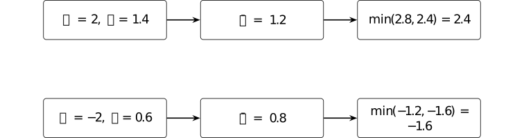
With \(\epsilon =0.2\), write \(\bar r=\operatorname {clip}(r,0.8,1.2)\) and \(L(r,A)=\min (rA,\bar rA)\). For positive advantage and \(r=1.4\), the gain is capped at \(2.4\). For negative advantage and \(r=0.6\), the clipped term \(-1.6\) is smaller than \(-1.2\), so the objective retains the penalty.

The pointwise surrogate comes from [schulman2017proximal, Section 3]. The two sign cases check only its arithmetic; they provide no monotone-improvement result for a neural policy or finite minibatch.

One prompt passes successively through supervised tuning, comparison-based reward modeling, and PPO in the InstructGPT-style RLHF pipeline.

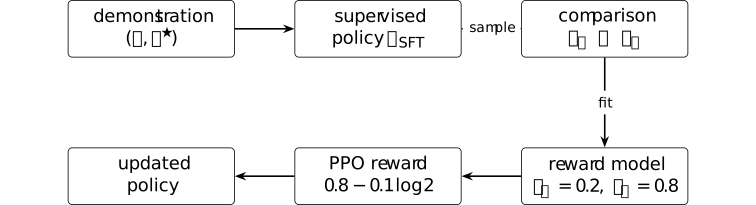
For the displayed illustrative prompt, suppose the comparison-trained reward model scores the preferred response by \(0.8\). If the candidate policy assigns it twice the probability assigned by the reference policy and the declared KL coefficient is \(\beta =0.1\), its shaped scalar is \[ 0.8-\beta \log \frac {\pi (y_B\mid x)} {\pi _{\rm ref}(y_B\mid x)} =0.8-0.1\log 2\approx 0.731. \]

The stage ordering is grounded in [ouyang2022training, Sections 3.1--3.5]; the numbers are a schematic calculation rather than reported InstructGPT hyperparameters. The diagram records the interface used in that pipeline. Other RLHF systems may order or replace the stages differently.

RLHF is a feedback-and-training pipeline; PPO is one optimizer used within that pipeline. PPO specifies a sampled update surrogate; it does not specify whose preferences are collected, what the reward means, or which independent behavior counts as aligned.

Changing the comparison population or reward model can change the alignment target while leaving PPO unchanged. Conversely, replacing PPO by another optimizer changes update geometry without necessarily changing the declared preference data or evaluation criterion.

Let \(\beta >0\) be the KL coefficient, \(\pi _{\mathrm {ref}}\) a fixed reference policy, and \(\pi _\theta \) a trainable policy with support contained in that of the reference on the responses under study. Define the reference-relative log likelihood

and, for a comparison observation, the paired difference

Direct preference training starts from a fixed reference policy and a dataset of preferred and dispreferred responses. It evaluates a binary cross-entropy loss formed from the trainable policy's reference-relative log likelihoods and updates the policy directly.

This stage does not separately fit a scalar reward network, sample online rollouts for PPO, or train a value function. Its loss nevertheless comes from a particular reward-model and KL-regularized optimization derivation.

For a reward \(r(x,y)\), reference policy \(\pi _{\mathrm {ref}}\), and \(\beta >0\), the optimizer of the per-prompt KL-regularized reward objective has the form

where

normalizes the policy on the response space. The identity assumes that the normalizer is finite and uses the same reference policy as the underlying objective.

Rearranging the optimal-policy identity of Definition 7.3 gives

The final term depends on the prompt but not on the response. It cancels from pairwise reward differences, matching the additive non-identifiability of Bradley--Terry scores described in Remark 3.9.

Substituting the reward--policy reparameterization into the Bradley--Terry law yields

where \(\Delta _\theta \) is defined in Notation 7.1. The prompt-dependent normalizer cancels because the two responses share the same prompt.

For comparison observations from \(\mathcal D_{\mathrm {pref}}\), the Direct Preference Optimization loss is

The empirical loss is evaluated on a fixed comparison dataset. The temperature, reference policy, record weights, and handling of ties or abstentions are part of the training specification.

Four declared policy probabilities determine the log-ratio margin in one DPO loss term.

Let \(\pi _\theta (y^+\mid x)=0.6\), \(\pi _{\rm ref}(y^+\mid x)=0.3\), \(\pi _\theta (y^-\mid x)=0.2\), and \(\pi _{\rm ref}(y^-\mid x)=0.4\). With \(\beta =1/2\), the DPO logit is \[ z=\beta \left [\log 2-\log (1/2)\right ] =\tfrac 12\log 4=\log 2. \] Hence \(\sigma (z)=2/3\) and the one-pair negative log-likelihood is \(-\log \sigma (z)=\log (3/2)\approx 0.405\).

Substitution into Equation (7) of [rafailov2023direct, Section 4] verifies one loss term. Consistency of the pairwise data, suitability of the reference policy, and improvement in independent utility are separate questions.

The derivation uses a fixed reference policy, a finite KL-regularized optimum, and a Bradley--Terry model for pairwise preferences. The relevant policy probabilities must be positive wherever their logarithmic ratios are evaluated.

The algebra eliminates the prompt-dependent reward offset, not every source of reward-model misspecification. Heterogeneous or nontransitive preferences, adaptive data collection, support mismatch, and finite-sample optimization remain separate questions.

DPO optimizes a policy directly on a fixed preference dataset. Reward-model PPO instead fits an explicit scalar reward predictor, generates policy rollouts, estimates advantages, and applies a policy-gradient update. DPO therefore removes the separately represented reward and online PPO loop from that training stage.

The methods still share ingredients: comparison data, a reference policy, a KL coefficient or temperature, and assumptions connecting comparisons with latent reward. Neither method defines preference optimization in general, and their data and compute requirements are not causally interchangeable.

An outcome-supervised reward model assigns a score to a complete response and is trained from labels attached to the final outcome. For a prompt \(x\) and completed response \(y\), write its score as

The training label states whether the completed solution reaches the declared outcome. It need not identify the first invalid step or distinguish a sound derivation from an answer reached for an unsound reason.

Suppose a response is segmented into reasoning steps \(y=(s_1,\ldots ,s_m)\). A process-supervised reward model produces a score for each declared prefix,

and is fitted from step-level labels. The segmentation rule and label semantics are part of the supervision: a score after step \(k\) need not be a decomposition of an outcome score for the whole response.

Outcome supervision uses one completed-response label, whereas process supervision supplies labels at declared intermediate steps. The latter can localize feedback, but it also requires a segmentation, a step-labeling criterion, and additional annotations.

Neither label type is automatically causal credit. A process label may be assigned after a reviewer has seen the whole response, and a terminal outcome may be predicted reliably from an early prefix without identifying which action should change.

Let \(\mathcal F_t\) be the sigma-algebra generated by the public history \(\mathsf H_t\) available through decision time \(t\). A feedback variable \(Z_t\) is online measurable at time \(t\) when it is \(\mathcal F_t\)-measurable and is delivered before the protocol chooses its next action.

A label computed only after observing a later action or terminal outcome is not online measurable at the earlier time, even if it is subsequently attached to that earlier prefix in the training data.

The index attached to a label does not determine when its information becomes available. The process-supervision construction in [lightman2023verify, Section 2.6] supplies step-indexed training labels, but it does not require every such label to be available while the response is being generated.

This distinction determines which interventions are admissible. An online agent may act on currently measurable feedback; an offline learner may use a post-hoc label for a past prefix; a causal claim needs assumptions connecting either signal to the consequences of the earlier action.

A four-step arithmetic trace can receive a correct terminal label while retaining an incorrect intermediate process label.

The final answer \(19\) is correct, so outcome supervision supplies \(f_{\rm out}=1\). The declared process labels are \((f_1,f_2,f_3,f_4)=(1,1,0,1)\) and expose the corrected arithmetic error at step three. The labels are attached to the displayed prefixes, which remain unchanged by those annotations.

The two supervision regimes follow the outcome- and process-supervised reward-model constructions in [lightman2023verify, the outcome- and process-supervised reward-model subsections]. The two observations are thereby separated. Noise-free labels and a general policy advantage for process supervision are not consequences of the finite trace.

Let \(\mathcal E\) be an evidence space. Write \(\mathsf V\) for a declared verifier, \(e_{\mathrm {ver}}\in \mathcal E\) for its evidence, \(d_{\mathrm {ver}}\in \{0,1\}\) for its decision, and \(R_{\mathrm {ver}}\in \mathbb R\) for the reward derived from that result.

For a prompt \(x\) and group size \(g\geq 2\), write \(\mathbf Y_x=(Y^{(1)},\ldots ,Y^{(g)})\) for a rollout group sampled from the behavior policy. Let \(R_i\) be the reward of member \(i\), \(\bar R\) the group mean, \(S_R\) the group standard deviation, and \(\widehat A_i\) its group-relative advantage.

Reinforcement learning with verifiable rewards is a post-training method that samples responses from a language-model policy, computes rewards with a deterministic check of the response, and applies a reinforcement-learning update to increase expected checked reward, optionally with regularization to a reference policy.

In the cited construction, a correct response receives reward \(\alpha \) and an incorrect response receives \(0\). Equation (8) gives this two-valued form, and the paragraph immediately after it sets \(\alpha =10\). The checked predicate, reward scale, prompt law, rollout procedure, and policy optimizer remain separate parts of the method.

Concrete RLVR methods include the PPO-based construction in [lambert2024tulu3, Section 6], group relative policy optimization (GRPO) in [shao2024deepseekmath, Section 4.1], R1-Zero in [guo2025deepseek, Section 2.2], and Decoupled Clip and Dynamic sAmpling Policy Optimization (DAPO) in [yu2025dapo, Sections 2--3].

A proposed common description groups methods that acquire policy samples, evaluate a declared verifiable signal, assign credit, and update the policy. A specific claim must still name its verifier, group sampling, estimator, clipping, normalization, reference-policy treatment, and length rule.

For prompts and responses from Notation 2.1, a deterministic verifier correctness indicator is a declared map

Here \(v(x,y)=1\) means that the response satisfies the checked predicate. The map includes the parsing and execution rules needed to reproduce the decision. A stochastic judge or learned reward model is a different feedback mechanism unless its randomness and decision procedure are separately exposed.

A verifier evidence record is a tuple

where \(\iota _{\mathrm {ver}}\) identifies the verifier and its version, \(o\) is the reproducible output used by the check, and \(d_{\mathrm {ver}}\in \{0,1\}\) is the resulting decision. Examples of \(o\) include a parsed exact answer, a test log, or a proof-checker result.

The evidence record preserves how the decision was obtained. It does not assert that the checked predicate is complete for the task's independent success criterion.

The same correctness decision can arise from different parsers, tests, proof kernels, or failure modes. Tülu 3 uses a scaled two-valued reward \(\alpha \) or \(0\), with \(\alpha =10\), in [lambert2024tulu3, Section 6, equation (8), and the immediately following paragraph]; it does not identify that reward with a complete record of the checking procedure.

Evidence enables later audits of false positives, false negatives, version changes, and shortcut exploitation. Reproducibility of the check still does not establish that the checked predicate equals the intended capability.

Given a deterministic correctness indicator \(v\) and reward scale \(\alpha >0\), the verifiable reward in the cited construction is

The paragraph after Equation (8) sets \(\alpha =10\). Another method may choose a different scale or combine several checked components, but that transformation is part of its reward design. A reward is verifiable relative to the implemented check, not relative to every property an independent evaluator may care about.

Rule evidence compares a parsed answer or format with a declared target, as in [guo2025deepseek, Section 2.2]. Test evidence executes a candidate in a sandbox and records test outcomes. Proof evidence submits a term to a specified checker and records acceptance or an error.

These routes expose different predicates and costs. A rule can ignore the derivation, a test suite can omit behavior, and a proof checker establishes only the proposition and trusted-kernel boundary it was given. Their rewards must not be merged without retaining which evidence source fired.

Fix a prompt \(x\), group size \(g\geq 2\), and behavior policy \(\pi _b\). A rollout group is the indexed family

DeepSeekMath samples several outputs for the same prompt so their rewards can define a group-relative baseline. The producing policy, decoder, group size, and conditional sampling dependence are part of the rollout law.

For rollout-group rewards \(R_1,\ldots ,R_g\), define the group mean and group standard deviation by

Both statistics are prompt-local and depend on every member of the sampled group. The source leaves the standard-deviation divisor symbolic and does not add a numerical stabilizer. An implementation must state those conventions and its treatment of zero-variance groups.

When \(S_R>0\), the group-relative advantage of rollout member \(i\) is

The estimator compares responses sampled for the same prompt and does not require a learned value function. Its members are statistically coupled through \(\bar R\) and \(S_R\); it is not an independent estimate of the population advantage of each response.

Outcome-supervision GRPO samples a group of responses for one prompt, assigns each response an outcome reward, standardizes those rewards within the group, and uses the resulting group-relative advantage across the response's token log-likelihood terms.

The construction removes a separately learned critic but retains a behavior policy, likelihood ratios, a reference-policy term in the source formulation, and explicit normalization choices.

Process-supervision GRPO supplies rewards at declared reasoning steps and forms advantages from the subsequent step rewards assigned to each token. The policy objective therefore receives credit that can vary within one response rather than repeating one terminal outcome advantage at every token.

This construction requires a step segmentation and a process reward model. Its estimator is not obtained merely by relabeling an outcome-supervision rollout group.

GRPO names a family of group-relative policy updates rather than one fully determined estimator. Outcome and process supervision assign different reward structures. Implementations may also differ in token versus response normalization, KL terms, clipping intervals, importance weights, and treatment of groups with zero reward variance.

A result about one variant must retain its producing policy and all of those conventions. Sharing the group-relative baseline does not make the resulting gradients identical.

Clip-higher replaces the symmetric upper and lower PPO clipping widths by separate constants. It permits a larger upward likelihood-ratio movement for tokens with positive advantage while retaining a smaller lower-side interval.

The change alters which sampled terms are saturated by the surrogate. It does not impose a policy-wide trust region or guarantee preservation of low-probability actions.

DAPO dynamic sampling filters prompt groups whose sampled responses all receive the same reward and continues sampling until the training batch contains the declared number of groups with nonzero reward variation.

The intervention changes the distribution of prompts and rollouts entering the update. It can prevent zero-advantage groups from consuming an optimizer batch, but the retained batch is no longer an unconditioned sample from the original prompt law.

The token-level loss aggregates active token terms across the complete minibatch and divides by the number of active tokens. A longer response therefore contributes in proportion to its active token count rather than receiving the same total weight as every shorter response.

This normalization changes the empirical gradient even when the sampled responses, rewards, advantages, and likelihood ratios are unchanged. It must be distinguished from averaging a separately normalized loss over responses.

Overlong reward shaping introduces a soft penalty near the maximum response length before the hard truncation boundary. The penalty increases over a declared buffer region rather than assigning the same abrupt terminal penalty to every response that reaches the limit.

The construction changes both the reward value and which length-related behavior receives gradient. The maximum length, buffer width, and penalty schedule are part of the reward design.

Clip-higher changes the saturated region of the policy surrogate, dynamic sampling conditions which prompt groups enter a batch, token-level aggregation changes response-length weighting, and overlong shaping changes the reward near a truncation boundary. These are four different interventions.

An observed training improvement cannot be assigned to a generic ``algorithm'' without an ablation that holds the other sampling, estimator, reward, and compute choices fixed. The interventions also change which rollouts and gradients are observed, so their effects need not add linearly.

Three sampled responses pass through exact verification, group credit, and a proposed update in one finite RLVR round.

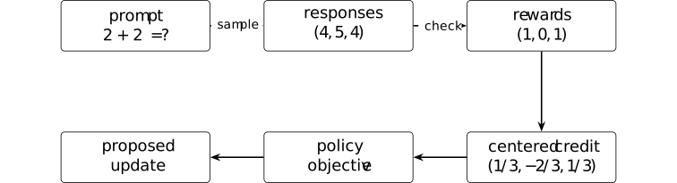
The exact-answer checker gives mean reward \(\bar r=2/3\). Using the declared unnormalized centered credit \(\widehat A_i=r_i-\bar r\) yields \((1/3,-2/3,1/3)\). An optimizer may use these numbers to propose a parameter change, but the tuple itself is not yet an accepted update.

The RLVR protocol is Definition 9.2. Its group-credit objects are Definition 9.9, Definition 9.10, and Definition 9.11. Together they specialize to this finite order of operations. Centered, unscaled credit and an exact-answer checker are local choices rather than requirements on other RLVR algorithms.

A rollout group is normalized to relative advantages and then passed to a clipped surrogate objective.

For a rollout group with rewards \(r_i\), form a group mean and scale and set \(\widehat A_i=(r_i-\bar r)/s\). For current-to-behaviour ratios \(\rho _i\) and clip interval \([1-\epsilon ,1+\epsilon ]\), define each pointwise term by

The mean of the resulting terms is the group contribution to the update; its value depends on the sampled rewards, ratios, and clip width.

Group-relative normalization is grounded in [shao2024deepseekmath, Section 4.1], while clipping is grounded in [schulman2017proximal, Section 3]. The normalization convention and ratios must be declared by the training protocol; a positive surrogate mean alone gives no guarantee of improved held-out performance after an optimizer step.

Fix the token vocabulary and strings of the tokenizer interface, and the action space \(\mathcal A\) from the declared interactive task realization. An action serializer is a pair of partial maps

The encoder gives an action a textual representation. The decoder recognizes a completed representation and returns the executable action. A string outside the decoder's domain is malformed; it is not silently promoted to an environment action. For every action in the encoder's domain, the declared pair satisfies \(\operatorname {dec}(\operatorname {enc}(a))=a\).

An action serializer maps generated text to an executable action. Section 2 of ReAct: Synergizing reasoning and acting in language models[yao2023react] writes actions and observations in a textual trajectory. The proposed serializer interface in Definition 10.1 additionally distinguishes malformed calls, constrained grammars, and environment actions.

An improvement can therefore come from better reasoning, better serialization, or a more permissive parser. These are separate intervention coordinates.

A ReAct interaction alternates model-generated reasoning and actions with observations returned by an external interface. The observation is appended to the next model context, so subsequent actions may depend on earlier tool results.

A decoded action belongs to \(\mathcal A\) in the declared interactive task realization; the transition--observation kernel of Definition [ftip-001Z] returns the next observation. The cited construction does not by itself fix a sandbox, reward, or training algorithm.

Fix an interactive realization \(\mathsf {Env}_{\mathsf T}\) from the declared task interface, a measurable evidence space \(\mathcal E_{\rm box}\), and a cost dimension \(m\geq 1\). A sandbox specifies an allowed action set \(\mathcal A^{\rm box}_{\mathsf T}\subseteq \mathcal A_{\mathsf T}\) that is measurable, a cost bound \(b_{\rm box}\in \mathbb R_+^m\), and, for each \(x\in \mathcal X_{\mathsf T}\) and \(0\leq t<T_{\max }\), an execution kernel

It also specifies, for each \(x\in \mathcal X_{\mathsf T}\), a reset kernel

For an allowed action, the state--observation marginal of \(K_t^{\rm box,x}\) is the kernel \(K_t^x\) in the task realization; the state--observation marginal of the reset kernel is \(\rho _0^x\). The remaining coordinates record reproducible evidence and a realized cost increment. An admitted stopped trajectory must have componentwise cumulative cost at most \(b_{\rm box}\).

The sandbox semantics include permissions, kernel and reset versions, evidence encoding, and cost accounting. A tool name or API schema alone does not determine these fields.

A sandbox restricts the environment through its executor, reset rules, permissions, and evidence. ReAct [yao2023react, Section 2] supplies the action--observation pattern. Software-agent systems surveyed in [wang2024agents, Section 2.3.2] add repositories, compilers, tests, and other digital tools. The combined sandbox interface is a proposed model of these choices.

Two protocols that share prompts but change reset or permission semantics need not induce the same trajectory law.

Let \(\mathcal M_{\rm exec}\) be the space of executable model artifacts, \(\mathcal Z_{\rm opt}\) the optimizer-state space, and \(\mathcal R_{\rm ag}\) a declared space of typed agentic round records. At training round \(n\), an agentic post-training state is a tuple \[ \Sigma _n=(M_n,s_n,\mathcal L_n) \in \mathcal M_{\rm exec}\times \mathcal Z_{\rm opt} \times \mathcal R_{\rm ag}^{n}, \] where \(M_n\) is the executable model artifact, \(s_n\) is the optimizer state, and \(\mathcal L_n=(r_0,\ldots ,r_{n-1})\) is an append-only training ledger.

The round-record schema records the task and instance draw, policy and inference stamp, environment version, stopped trajectory, feedback and credit outputs, update decision, proposed and committed next artifact and optimizer state, random seeds, operator versions, and realized cost vector. The tuple separates executable state from optimizer state and from evidence about how that state was reached.

At round \(n\), fix a task \(\mathsf T_n\), its law \(\mu _{\mathsf T_n}\), and a versioned interactive realization \(\mathsf {Env}^{\upsilon _n}_{\mathsf T_n}\). Let \(\mathcal I_{\rm art}\) and \(\mathcal I_{\rm inf}\) be declared identifier spaces. Let \(a_n\in \mathcal I_{\rm art}\) be an immutable content identifier resolving the artifact \(M_n\), and let \(\iota _n\in \mathcal I_{\rm inf}\) record all serializer, decoding, tool, and stopping settings. The policy--inference stamp \(\nu _n=(a_n,\iota _n)\in \mathcal I_{\rm art}\times \mathcal I_{\rm inf}\) resolves a non-anticipating policy \(\pi _n\). Let \(\Omega _n^{\rm task}\), \(\Omega _n^{\rm roll}\), \(\Omega _n^{\rm feed}\), \(\Omega _n^{\rm credit}\), and \(\Omega _n^{\rm update}\) be declared seed spaces. The rollout seed contains both policy-decoding and environment randomness. Write \(\Omega _n=\Omega _n^{\rm task}\times \Omega _n^{\rm roll}\times \Omega _n^{\rm feed}\times \Omega _n^{\rm credit}\times \Omega _n^{\rm update}\), and let \(\omega _n=(\omega _n^{\rm task},\omega _n^{\rm roll}, \omega _n^{\rm feed},\omega _n^{\rm credit},\omega _n^{\rm update})\) be sampled from a declared joint law on \(\Omega _n\). Write \(\mathcal Z_{\mathsf T_n}\) for the stopped trajectories admitted by the versioned realization.

For declared feedback and credit spaces \(\mathcal F_n\) and \(\mathcal G_n\), decision space \(\mathcal D_n=\{\mathsf {accept},\mathsf {reject}\}\), accounting dimension \(m\geq 1\), and exact implementation versions \(v_n^{\rm S}\), \(v_n^{\rm R}\), \(v_n^{\rm F}\), \(v_n^{\rm C}\), \(v_n^{\rm U}\), and \(v_n^{\rm A}\), the round specifies maps

The accounting map receives the starting state, proposed state, decision, and realized seeds, so update work and rejected proposals remain observable in the cost record.

They produce

The task sampler pushes its seed law forward to \(\mu _{\mathsf T_n}\). Conditional on \(X_n\), the rollout sampler pushes its seed law forward to the interaction law of Remark [ftip-0028] under \(\mathsf {Env}^{\upsilon _n}_{\mathsf T_n}\) and \(\pi _n\).

If \(d_n=\mathsf {accept}\), set \((M_{n+1},s_{n+1})=(\widetilde M_{n+1},\widetilde s_{n+1})\); if \(d_n=\mathsf {reject}\), set \((M_{n+1},s_{n+1})=(M_n,s_n)\). The realized cost \(c_n\) includes proposal work even after rejection. With \(v_n^{\rm ops}=(v_n^{\rm S},v_n^{\rm R},v_n^{\rm F},v_n^{\rm C}, v_n^{\rm U},v_n^{\rm A})\), append

The record belongs to \(\mathcal R_{\rm ag}\) from Definition 10.6 and determines \(\Sigma _{n+1}\) without rewriting an earlier record.

An agentic post-training run fixes a finite round count \(N_{\rm ag}\geq 0\), an initial state \(\Sigma _0\), a fixed accounting dimension \(m\geq 1\), a componentwise budget \(b_{\rm ag}\in \mathbb R_+^m\), and the round specifications of Definition 10.7. Put \(\Omega _{\rm ag}=\prod _{n=0}^{N_{\rm ag}-1}\Omega _n\), using a singleton for the empty product. Once those specifications and their exact versions \(v_{\rm ag}\) are fixed, the run is the map

Write a realized round-seed tuple as

The run recursively constructs \(\Sigma _1,\ldots ,\Sigma _{N_{\rm ag}}\); the seed tuple and state sequence are empty beyond \(\Sigma _0\) when \(N_{\rm ag}=0\). Its cumulative realized cost is \[ c_{\rm ag}=\sum _{n=0}^{N_{\rm ag}-1}c_n. \] The empty sum is \(0\in \mathbb R_+^m\) when \(N_{\rm ag}=0\). The map returns \((M_{N_{\rm ag}},\mathcal L_{N_{\rm ag}},c_{\rm ag})\). A run claiming the hard budget must declare a pre-admission or stopping rule that guarantees \(c_{\rm ag}\preceq b_{\rm ag}\).

The run declaration includes the task sampler, environments, serializers, rollout inference settings, feedback and credit maps, update maps, stopping rule, seed laws, implementation versions, and resource account. The round records retain every realized seed, version, decision, and cost. Leaving one of these fields implicit defines a family of runs rather than one reproducible intervention.

A proposed interactive extension of the response-level RLVR cycle in § 9 uses the environment of § [ftip-001W] and the action boundary of Definition 10.1. It retains intermediate observations and environment state instead of treating a whole response as one indivisible action.

This change introduces new questions about partial observability, long-horizon credit, environment versioning, recovery after interruption, and the cost of external execution. It does not assert that multi-turn training is uniformly better than response-level training.

A failing test observation triggers a second edit, whose passing tool evidence determines the terminal result.

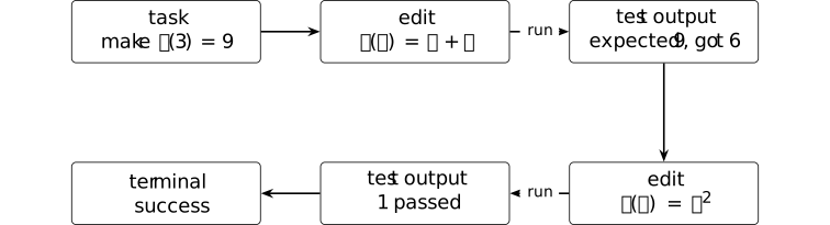
The public history records both edits and both test outputs. The first tool call returns the evidence string expected 9, got 6; the second returns exit status \(0\) and 1 passed. The success rule reads the second test result rather than the model's assertion that its edit is correct.

The action--observation alternation follows the tool-interleaving pattern in [yao2023react, Section 2]. The transparent sandbox interaction certifies only the displayed test result; completeness of the suite and satisfaction of unstated intent remain unverified.

Two coupled panels place resumable generation beside sandbox evidence in a single rollout record.

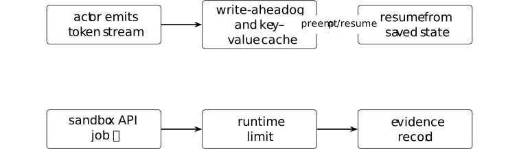
A write-ahead log and cached state allow a resumable rollout; a sandbox execution contributes a separately recorded evidence tuple. The two records should remain distinguishable when lifecycle cost is audited.

Token-granular write-ahead logging with key--value cache recovery and DeepSeek Elastic Compute (DSec), the report's named sandbox interface, are described in Sections 5.2.3 and 5.2.5 of the DeepSeek-V4 family report [⧉]. The cited sources do not establish that DeepSeek-V4-Flash-0731 used this job, resource limit, rollout schedule, or sandbox configuration.

A policy stamp \(\nu \) is a content-addressed description of an executable policy: model artifact, tokenizer, action serializer, decoding settings, and implementation revision. Resolving the stamp produces the action law \(\pi ^\nu (\,\cdot \mid \mathsf H_t)\) for every public history in its declared domain.

Two stamps are equal only when every component that may change the action law is equal. A display name or checkpoint step is therefore insufficient.

Off-policy methods distinguish the behavior and current policies, while language-model artifacts also depend on tokenization and decoding. Section 3 of When to stop reusing: Dynamic gradient gating for sample-efficient RLVR[miao2026when] records the behavior/current distinction. The additional artifact and implementation fields in the proposed policy stamp make the executable law reproducible.

The stamp identifies an executable law; it does not claim that two implementations with different stamps must behave differently on every task.

An immutable rollout record is a tuple

where \(q\) is the sampled task, \(\nu _b\) is the behavior-policy stamp, \(\tau \) is the stopped trajectory of Definition [ftip-0025], and \(e\) is the verifier evidence of Definition 9.5. The tuple records facts fixed when the rollout finishes.

Current-policy likelihood ratios, clipping decisions, reuse counts, and acceptance decisions are excluded because they may change on a later update attempt.

An immutable historical record prevents an update attempt from rewriting the facts attached to its reused samples. The sample-reuse setup in [miao2026when, Section 3] retains behavior-policy rollouts while recomputing current-policy ratios. Dynamic Gradient Gating (DGG), defined in [miao2026when, Section 5 and Algorithm 1], is one such reuse protocol, while the complete immutable tuple is a proposed interface for such protocols.

Recorded facts and estimates recomputed for an attempted update are different objects; errors in the latter do not alter the former.

Let \(\mathcal R\) be the set of immutable rollout records and \(\mathcal F\) a typed set of feedback events. A feedback operator is a possibly randomized kernel

A feedback event may contain an outcome score, step labels, a preference, or an abstention. Its type records which observations were available when it was produced.

Let \(R\) be a rollout record with \(\tau _{\rm stop}\) actions, and let \(f\) be its feedback event. A credit-assignment rule returns indexed training targets

Each \(c_t\) is attached to an action or token position declared by the rule. It may be a return, an advantage estimate, a binary label, or a structured target. The rule is distinct from the feedback source that supplied \(f\).

Terminal returns, process labels, preference observations, and verifier rewards determine what information is observed. A credit rule determines where that information enters an objective. Treating them as separate inputs is a proposed common description of these different methods.

Separating the interfaces permits questions about delayed, noisy, or misallocated credit without changing the underlying evidence.

At update index \(n\), a replay pool \(\mathcal R_n\) is a finite multiset of immutable rollout records eligible for selection. Its management rule specifies insertion, eviction, and any partition by task or behavior stamp.

The pool is persistent state of the training protocol. It is not the minibatch selected for one update.

Selecting \(R\in \mathcal R_n\) under a current policy stamp \(\nu _n\) produces an attempt-local replay annotation

where \(\rho \) is the declared collection of behavior/current likelihood ratios, \(\kappa \) records clipping status, \(m\) is the record age, and \(u\) is its prior reuse count. Every component is computed for this attempt and may change at the next one.

The proposed replay interface separates a persistent pool from annotations computed for an update attempt. DGG in [miao2026when, Section 3; Section 5 and Algorithm 1] recomputes policy ratios and a gradient diagnostic while reusing a rollout batch. Those quantities depend on the current policy and therefore belong to the attempted update rather than the historical record.

The split also exposes the cost of selecting, scoring, and rejecting reused records.

Reusing one historical rollout recomputes current-policy annotations without mutating the stored record.

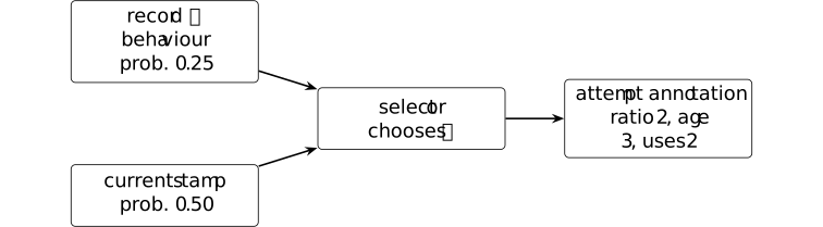
Let the stored record be \(R=(q,\nu _b,\tau ,e)\) and suppose its behaviour policy assigned the recorded action probability \(0.25\). Under the current stamp the same action has probability \(0.50\), so this attempt records importance ratio \(0.50/0.25=2\). Its age \(3\) and prior-use count \(2\) are also attempt-time metadata; none of these three values rewrites \(R\).

The behaviour/current-policy distinction is required by the reuse analysis in [miao2026when, Section 3]. The finite annotation makes provenance explicit. Statistical safety of ratio \(2\), age \(3\), or a second reuse is left undecided.

Given a current parameter--optimizer state \((\theta _n,z_n)\), selected records, their attempt annotations, and credit targets, an update proposal is a candidate next state

The diagnostic record \(\delta _n^{\rm diag}\) contains the quantities required by the declared acceptance rule. It is distinct from the accept--reject decision \(d_n\) recorded for the proposal. Constructing the proposal incurs update cost even if the proposal is later rejected.

Dynamic gradient gating computes the language-model-head gradient before the optimizer step. It compares the change in squared Frobenius norm with a trailing-window Z-score. When the score crosses its threshold after a reused update, the method discards that gradient and returns to fresh rollouts.

The gate is an empirical stopping rule for reuse. The source does not prove that its Z-score is a calibrated divergence test or a general safety certificate.

A gate may reject a computed gradient even though its computation has already consumed resources. The DGG definition in Definition 11.13 supplies the motivating pre-optimizer discard operation. Other protocols may inspect held-out loss, divergence, or resource limits.

The generic proposal interface does not transfer DGG's empirical detector to those other diagnostics. Each gate needs its own assumptions and calibration evidence.

Two candidate reused-gradient updates fall on opposite sides of a declared DGG-style gate.

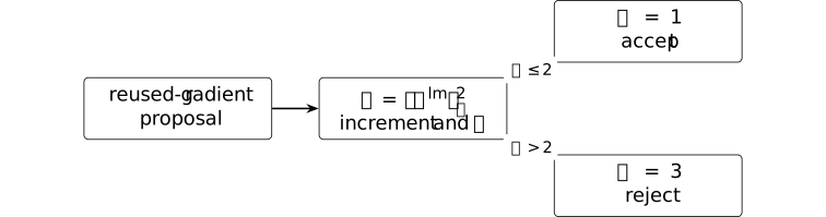
Declare a trailing-window increment mean \(\mu =1\), standard deviation \(s=0.5\), and toy threshold \(z_\star =2\). Proposal A has increment \(1.5\), so \(Z_A=(1.5-1)/0.5=1\) and is committed. Proposal B has increment \(2.5\), so \(Z_B=3\) and is rejected before an Adam transition. Rejection therefore leaves both parameters and optimizer moments unchanged in this protocol.

The monitored last-layer gradient energy, trailing-window Z-score, and pre-optimizer rejection order are modeled on [miao2026when, Section 5 and Algorithm 1]; the numeric threshold and window statistics above are locally declared. Acceptance is a reuse heuristic; it supplies neither a safety certificate nor a guarantee of improved independent evaluation.

NExt forms global and local parameter differences from saved low-rank adaptation (LoRA) checkpoints, approximates each matrix difference by leading singular factors, and trains a predictor on those representations to estimate a future difference. It adds a scaled predicted difference to a checkpoint; the reported experiments then resume RLVR updates.

The construction replaces some realized rollout-and-update steps with a learned parameter jump. It does not introduce a new verifier signal.

The NExt construction Low-rank optimization trajectories modeling for LLM RLVR acceleration[chen2026lowrank] motivates a distinction between following a predictable parameter path and acquiring information from new rollouts. Low-rank dominance of saved differences does not imply linear future motion, invariance across parameterizations, or preservation of optimizer state.

A cost comparison includes checkpoint storage, decomposition, predictor training, extrapolation, and recovery updates. Bounding independent-evaluation regret additionally requires stability assumptions connecting parameter forecasts to the evaluated outcome.

Leading rank-one projectors encode a checkpoint direction without inheriting the arbitrary signs of singular vectors.

For either singular-vector representation \((u,v)\) or \((-u,-v)\), the projectors \(P_u=uu^\top \) and \(P_v=vv^\top \) are unchanged. A trajectory forecaster can extrapolate the observed projector-aligned deltas to a next checkpoint, after which a measured recovery update can correct the forecast without changing the represented one-dimensional subspace.

The history-to-delta-to-recovery order is a toy illustration of NExt, described in [⧉]. NExt models signed singular value decomposition (SVD) factors rather than the projector construction used here. Accordingly, the calculation supplies neither a theorem about checkpoint trajectories nor evidence of capability acquisition.