Fix a sampled history and an active token \(i\) in the interior of the unclipped branch of the GRPO objective. Consider a finite directed acyclic computation graph that is differentiable at the parameter point in question. Let \(a_i\) be the sampled token, \(\widehat A_i\) its fixed normalized advantage, and \(p_i=\operatorname {softmax}(z_i)\) the current distribution on a finite vocabulary \(\mathcal V\). With fixed behavior probability \(b_i>0\), set \[ r_i=\frac {p_i(a_i)}{b_i}, \qquad \mathcal L_i=r_i\widehat A_i, \qquad E_i=r_i\widehat A_i(e_{a_i}-p_i). \] Here \(e_{a_i}\in \mathbb R^{|\mathcal V|}\) is the sampled-token basis vector. The history and sampling decisions are held fixed during differentiation.

Suppose the output head \(W_{\rm lm}\in \mathbb R^{|\mathcal V|\times d_{\rm model}}\) is untied: its only path to \(\mathcal L_i\) is through \(z_i=W_{\rm lm}h_{L,i}\), and \(h_{L,i}\in \mathbb R^{d_{\rm model}}\) is independent of \(W_{\rm lm}\). Then \[ G_i^{\rm lm}=\nabla _{W_{\rm lm}}\mathcal L_i =E_i h_{L,i}^{\mathsf T}. \]

Let \(W_{\rm int}\in \mathbb R^{m\times d}\) be a shared intermediate weight. Index by a finite set \(\mathcal O_i\) every occurrence of this weight that can affect \(z_i\), assuming that all such uses have the form \(y_o=W_{\rm int}x_o\), with \(x_o\in \mathbb R^d\). First replace these uses by independent copies \(W_o\) and evaluate them all at \(W_o=W_{\rm int}\). Let \(J_{io}\in \mathbb R^{|\mathcal V|\times m}\) be the downstream Jacobian from node \(y_o\) to \(z_i\) in this graph, with the other weight copies fixed. Define the contribution of occurrence \(o\) by \[ H_{io}=\nabla _{W_o}\mathcal L_i =(J_{io}^{\mathsf T}E_i)x_o^{\mathsf T}. \] On tying the copies, the total derivative is \[ G_i^{\rm int}=\nabla _{W_{\rm int}}\mathcal L_i =\sum _{o\in \mathcal O_i}H_{io}. \] The head gradient and each occurrence contribution have rank at most one; the total shared-weight gradient need not.

For a layer used once per position in a causal network, the sum includes every earlier position whose output affects token \(i\). Reuse across depth adds further occurrences. Tying the head to embeddings or other blocks also requires their contributions; the displayed head identity assumes that such tying is absent.

Clipped or inactive terms require their own derivative or mask. [miao2026when, Section 4.2.1, Proposition 1, and Appendix A.1] derives the intermediate outer product through one local application. For a shared weight, that calculation gives \(H_{io}\); identifying it with the total \(G_i^{\rm int}\) omits the other occurrences. The sum above supplies the chain rule needed for shared parameters.

Use the per-token quantities and untied head of Theorem 1, and fix one occurrence \(o\in \mathcal O_i\). Assume \(d_{\rm model}\geq 1\) and positive constants \(\alpha _{\min }\), \(\beta _{\max }\), and \(C\) satisfy \[ \|h_{L,i}\|_2^2\geq \alpha _{\min }d_{\rm model}, \qquad \|x_o\|_2^2\leq \beta _{\max }d_{\rm model}, \] and the two logit-sensitivity bounds \[ \mathbb E_{a\sim p_i} \|(J_{io})_{a,:}\|_2^2\leq C, \qquad \|(J_{io})_{a_i,:}\|_2^2\leq C. \] If \(\widehat A_i\neq 0\) and \(p_i(a_i)<1\), then \[ \frac {\|H_{io}\|_F^2}{\|G_i^{\rm lm}\|_F^2} \leq \frac {\mathcal C_{\rm occ}} {(1-p_i(a_i))^2}, \qquad \mathcal C_{\rm occ} =\frac {4\beta _{\max }C}{\alpha _{\min }}. \]

This bounds one occurrence contribution, not the total derivative of a shared intermediate weight. For the latter, the sum in Theorem 1 gives only \[ \|G_i^{\rm int}\|_F \leq \sum _{o\in \mathcal O_i} \|J_{io}^{\mathsf T}E_i\|_2\|x_o\|_2. \] If the same displayed hypotheses hold for every occurrence, the triangle inequality yields the ratio bound \(|\mathcal O_i|^2\mathcal C_{\rm occ}/(1-p_i(a_i))^2\) for \(\|G_i^{\rm int}\|_F^2/\|G_i^{\rm lm}\|_F^2\). Controlling only the application at position \(i\) does not establish this all-occurrence hypothesis or the source's claimed bound for the total gradient. The contributing positions, reuse pattern, and Jacobians depend on the architecture. Neither bound establishes a small gradient or an evaluation-score comparison.

The activation and row-energy hypotheses and the local inequality follow the calculation in [miao2026when, Section 4.2.1, Lemma 1, Assumption 1, Theorem 1, and Appendix A.3], with the differentiated object restricted to an occurrence contribution. They do not prove the source's total shared-weight claim under its local hypotheses.

For \(T\geq 1\) active, unclipped tokens with fixed sampled histories and the untied output head of Theorem 1, let \[ G^{\rm lm}=\frac 1T\sum _{i=1}^T G_i^{\rm lm}, \qquad \overline {r^2}=\frac 1T\sum _{i=1}^T r_i^2, \] and set \[ c_{\max }= \max _{1\leq i\leq T} \widehat A_i^2 \|e_{a_i}-\pi _\theta (\mathord \cdot \mid h_{L,i})\|_2^2 \|h_{L,i}\|_2^2. \] Then \[ \|G^{\rm lm}\|_F^2\leq c_{\max }\overline {r^2} =c_{\max }(1+\widehat \chi ^2), \] where \(\widehat \chi ^2\) is the statistic of Definition [ftip-0066]. If \(c_{\max }>0\), rearrangement gives the source's equivalent direction \[ \widehat \chi ^2\geq \frac {\|G^{\rm lm}\|_F^2}{c_{\max }}-1. \]

The inequality points from observed head-gradient energy to a lower bound on this finite-batch squared-ratio statistic. It is not a converse: cancellation can hide nonunit ratios. The active cancellation example in Example 6 states its clipping interval explicitly. The proof uses no intermediate-weight bound.

The finite-batch inequality follows the calculation in [miao2026when, Section 4.2.2, Lemma 2, Theorem 2, and Appendix B], under the untied-head and fixed-history assumptions stated above.

The identities in Theorem 1--Theorem 3 concern gradients, importance ratios, activations, and occurrence-specific logit Jacobians. The intermediate bound controls a local contribution; a shared-weight bound needs control over all contributing occurrences. None of their hypotheses mentions the fixed independent-evaluation functional \(J_{\rm ev}\) of Definition [ftip-005E]. They therefore cannot imply that accepting an update preserves \(J_{\rm ev}\), or that rejecting one would have prevented a decrease.

DGG adds an empirical policy on top of those identities: it monitors the increment in head-gradient energy, standardizes that increment against a trailing window, and rejects some reused updates before the optimizer step [miao2026when, Section 5 and Algorithm 1]. Its reported experiments relate that policy to observed training stability. They do not turn the Z-score into a calibrated test of independent-evaluation safety.

Take one observed action \(a\) with \(\pi _{\rm old}(a)=1/2\) and \(\pi _\theta (a)=1/4\). The batch contains only that action, so \(T=1\) and \(r_1=1/2\). Hence \[ \widehat \chi ^2=r_1^2-1=-\frac 34. \] Both policies can be completed on a two-action space by assigning their remaining mass to the other action.

Thus the finite-batch statistic in Definition [ftip-0066] need not share the nonnegativity of the population Pearson divergence. Theorem Theorem 3 remains valid: its right side contains \(1+\widehat \chi ^2=1/4=\overline {r^2}\).

Fix \(\epsilon _{\rm clip}\in (0,1)\) and \(1<R<1+\epsilon _{\rm clip}\). On a two-token vocabulary, let both observed tokens have \(a_i=1\), current probability \(\pi _\theta (1)=1/2\), and behavior probability \(\pi _{\rm old}(1)=1/(2R)\). Take scalar hidden states \(h_{L,1}=h_{L,2}=1\) and fixed normalized advantages \(\widehat A_1=1\), \(\widehat A_2=-1\). These may be selected token terms from different rollout members. An untied head with both logits zero realizes the current probabilities. Both terms lie strictly inside the clipping interval of Definition [ftip-003F], so the clipped surrogate locally agrees with \(\mathcal L_i=r_i\widehat A_i\). Thus \(r_1=r_2=R\), and Theorem 1 gives \[ G_1^{\rm lm}=R(1/2,-1/2)^{\mathsf T}, \qquad G_2^{\rm lm}=-G_1^{\rm lm}. \] Consequently \(G^{\rm lm}=0\), while \(\widehat \chi ^2=R^2-1>0\). For this fixed clipping rule, the statistic in this construction is bounded above by \((1+\epsilon _{\rm clip})^2-1\).

For the raw surrogate \(\mathcal L_i=r_i\widehat A_i\) considered as a separate objective, the same algebra works at every \(R>1\) and yields arbitrarily large squared-ratio excess. This does not extend the active construction to arbitrary \(R\) under clipping: when \(R>1+\epsilon _{\rm clip}\), the positive-advantage term is locally constant, while the negative term remains active. Their clipped gradients are then \(0\) and \(-R(1/2,-1/2)^{\mathsf T}\), with nonzero mean \((-R/4,R/4)^{\mathsf T}\).

The example does not contradict Theorem 3: that theorem upper-bounds batch-gradient energy by a ratio moment. It supplies no lower bound on the gradient and no converse from zero batch-gradient energy to ratios equal to one. The arbitrary-ratio version concerns only the separate raw surrogate.

Let two consecutive proposed reused updates have the same monitored energy, \(g_{t-1}=g_t=1\). With trailing-window increment mean \(\mu _t=0\), any positive scale \(\sigma _t+\varepsilon \), and any positive threshold, DGG's score is \[ z_t=\frac {(g_t-g_{t-1})-\mu _t}{\sigma _t+\varepsilon }=0, \] so the gate accepts the proposal. Now choose a fixed evaluation interface for which the artifact before the accepted update has performance \(J_{\rm ev}=1\) and the artifact after it has performance \(J_{\rm ev}=0\).

This is consistent because the gate rule of Definition [ftip-005A] imposes no mathematical relation between its scalar monitor and \(J_{\rm ev}\). A safety claim would need an additional assumption connecting proposed updates to the independent evaluation law; the Z-score calculation alone cannot provide it.

Let \(\Delta W\in \mathbb R^{m\times n}\) be nonzero, set \(q=\min (m,n)\), and order its singular values as \(\sigma _1\geq \cdots \geq \sigma _q\geq 0\). Its leading squared singular-energy share is \[ \rho _1(\Delta W) =\frac {\sigma _1(\Delta W)^2}{\sum _{j=1}^q\sigma _j(\Delta W)^2} =\frac {\sigma _1(\Delta W)^2}{\|\Delta W\|_F^2}. \] The nonzero hypothesis prevents an undefined \(0/0\); the value lies in \([1/q,1]\).

NExt instead reports \(E_1=\sigma _1/\sum _j\sigma _j\) in Section 3.2 Low-rank optimization trajectories modeling for LLM RLVR acceleration[chen2026lowrank]. That nuclear-share statistic and \(\rho _1\) answer different questions. The squared share measures contribution to squared Frobenius norm.

For \(\Delta W\in \mathbb R^{m\times n}\) with \(q=\min (m,n)\geq 2\), its leading spectral gap is \[ \operatorname {gap}_1(\Delta W) =\sigma _1(\Delta W)-\sigma _2(\Delta W). \] A positive gap makes the leading left and right one-dimensional singular subspaces unique, although each chosen singular vector still has an arbitrary sign. When the gap is zero, a single leading vector is not intrinsic.

The quantity is undefined when \(q=1\), since there is no second singular value. Projector comparisons require a positive gap at every compared checkpoint.

Let \(\Delta W_t\) and \(\Delta W_s\) be nonzero matrices of the same shape, each with positive leading spectral gap. If \(u_1(t)\) and \(u_1(s)\) are unit leading left singular vectors, define their leading-subspace projector drift by \[ d_{\rm proj}(t,s) =\|\Pi _t^{\rm svd}-\Pi _s^{\rm svd}\|_F, \qquad \Pi _t^{\rm svd}=u_1(t)u_1(t)^{\mathsf T}, \quad \Pi _s^{\rm svd}=u_1(s)u_1(s)^{\mathsf T}. \] The definition is independent of both singular-vector signs and takes values in \([0,\sqrt {2}]\).

This is an additional proposed trajectory diagnostic; NExt does not define it.

A large value of \(\rho _1\) from Definition 8 says that one singular mode dominates a particular difference matrix. It does not say that the dominant subspace remains fixed across checkpoints; \(d_{\rm proj}\) measures that separate question.

Fix the evaluation interface of Convention [ftip-005D]. Let \(P_{t+s}^{\rm act}\) be the protocol that returns the artifact reached after \(s\geq 1\) additional realized training steps from checkpoint \(t\). Let \(\mathcal K_{\leq t}\) be the saved checkpoint history available through \(t\), and let \(\widehat P_{t+s}(\mathcal K_{\leq t})\) instead return the artifact forecast from that history. Their signed path-emulation regret and absolute path-emulation regret are \[ \begin {aligned} \operatorname {Reg}^{\rm path}_{\rm ev}(t,s) &=J_{\rm ev}(P_{t+s}^{\rm act}) -J_{\rm ev}(\widehat P_{t+s}(\mathcal K_{\leq t})),\\ \operatorname {AReg}^{\rm path}_{\rm ev}(t,s) &=\left |\operatorname {Reg}^{\rm path}_{\rm ev}(t,s)\right |. \end {aligned} \]

The sign distinguishes an optimistic forecast from a pessimistic one; the absolute value measures discrepancy without cancellation across checkpoints. Both use the same task law, inference budget, and evaluator. Parameter error alone is not substituted for evaluation error. The NExt extrapolation and recovery schedule described in Sections 4.1--4.3 and 5.1 motivates this comparison Low-rank optimization trajectories modeling for LLM RLVR acceleration[chen2026lowrank], but the paper does not state this regret definition.

Let \(e_1=(1,0)^{\mathsf T}\) and \(e_2=(0,1)^{\mathsf T}\) be the standard basis vectors of \(\mathbb R^2\). In a two-dimensional matrix chart, set \(P=e_1e_1^{\mathsf T}\) and \(Q=e_2e_2^{\mathsf T}\). Two paths share the entire observed history \[ W_0=0,\qquad W_1=P,\qquad W_2=2P. \] Every observed local difference is the same rank-one matrix \(P\). The paths then fork: path A takes \(W_3^A=3P\), whereas path B takes \(W_3^B=2P+Q\). Each next local difference is again rank one.

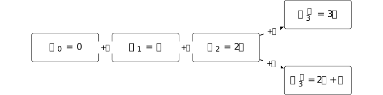
A deterministic history-only forecaster must return the same matrix \(\widehat W_3\) in both worlds. Since \(\|W_3^A-W_3^B\|_F=\|P-Q\|_F=\sqrt {2}\), the triangle inequality forces its Frobenius error to be at least \(1/\sqrt {2}\) on one continuation. Low-rank early motion therefore does not identify the next subspace or the next checkpoint.

NExt extracts global, local, and target differences from LoRA checkpoint matrices, keeps leading singular factors, learns a nonlinear predictor, jumps in that parameter chart, and resumes RLVR [chen2026lowrank, Sections 3.2, 4.1--4.3, and 5.1]. Its reported results are empirical; the paper states no theorem that a leading subspace remains stable or that a forecast preserves a policy.

The quantities in Definition 8--Definition 11 separate four tests. Squared singular-energy share concerns one matrix, spectral gap controls whether its leading subspace is identifiable, projector drift compares those subspaces over time, and path-emulation regret returns to fixed independent evaluation. None, by itself, is evidence that new feedback was acquired or that a new capability was learned. Such a claim must use a declared post-training gain such as Definition [ftip-005F] and must charge forecast training, the parameter jump, and recovery updates.