[clay2026demystifying, Sections 4.1--4.3 and Figure 1] organize the reported experiments along three declared axes: a starting model distribution, a training-prompt distribution, and a reward function. Each reported measurement therefore belongs to a cell of a matrix rather than to an unqualified ``RL post-training'' condition. The source holds its broad training recipe fixed while varying selected axes; it does not study variation among RL algorithms.

Each experimental comparison is conditional on its model, task, prompt law, executable reward rule, training budget, and evaluation procedure. The reward rule is especially consequential here because the main text and Appendix C do not state identical sparse-reward semantics. Section 4.2 describes target containment with a length penalty. Appendix C's prose says an exact target receives unit reward, but its displayed equation requires the response to be strictly longer than the target for any positive reward. These two descriptions do not identify a single sparse-reward implementation.

Fix an evaluation instance \(x\), a response space \(\mathcal Y_x\), and a declared target predicate \(h_x^\star :\mathcal Y_x\to \{0,1\}\). For a sampled response \(Y\), the target-response event is

The predicate is part of the evaluation specification. It may test exact string equality after a declared normalization, containment of a target substring, equality of a parsed answer, or another explicitly typed condition. These predicates are not interchangeable. The movie-quote and AIME experiments in [clay2026demystifying, Sections 4.1--4.2] use different response objects and therefore require different target predicates.

Let \(y_x^\star \) be a designated string and let \(N_x\) be a declared normalizer. Exact-string success is the specialization \(h_x^\star (y)=\mathbf 1\{N_x(y)=N_x(y_x^\star )\}\) of Definition 1.2. A task utility may instead accept semantically equivalent answers, assign partial credit, invoke a verifier, or depend on evaluator randomness as in Convention [ftip-005D].

Consequently, a change in target-string match rate is not automatically a change in task utility. [clay2026demystifying, Sections 4.1--4.2] deliberately use narrow target behaviours to study controlled coverage. Transferring their measurements to broader capability requires a separately justified evaluator.

For one declared model family and target predicate, a starting-policy triple is

Here \(\pi ^{\mathrm {base}}\) is the unmodified starting policy, \(\pi ^+\) is obtained by a declared supervised update intended to increase target-response frequency, and \(\pi ^-\) is obtained by a declared update intended to decrease it. The superscripts name producing interventions, not mathematical order relations between the resulting policies.

[clay2026demystifying, Section 4.1] instantiates the triple with the source's Base, SFT-positive, and SFT-negative checkpoints. For the movie quote, its SFT mixture places twenty percent weight on the target quote and eighty percent on other quotes from the Cornell Movie-Dialogs corpus; the negative intervention maximizes cross-entropy loss on the target.

The policies \(\pi ^+\) and \(\pi ^-\) of Definition 1.4 are produced by optimization. Their weights, output probabilities, representations, and off-target behaviours can all change together. Calling one intervention ``positive'' and the other ``negative'' describes its intended effect on the declared target response; it does not assert that only one probability mass was edited.

The comparisons in [clay2026demystifying, Sections 4.1 and 5.1] therefore test dependence on three constructed starting checkpoints. They do not identify a causal effect of initial target probability alone without an additional intervention model.

A controlled post-training experiment cell is a record

where \(M\) identifies the model architecture and checkpoint lineage, \(\pi ^{\mathrm {init}}\) is its starting policy, \(\mathsf T\) is the task, \(\mathcal D_{\mathrm {tr}}\) is the training-prompt law, \(r^{\mathrm {id}}\) identifies an executable reward rule and version, \(\mathcal A\) is the update procedure, \(b_{\mathrm {tr}}\) is the training budget, and \(\mathsf E\) is the evaluation interface. Random seeds and hyperparameters belong to the relevant record fields even when suppressed from the notation.

[clay2026demystifying, Figure 1 and Sections 4.1--4.3] motivates the coordinates. The source varies starting distribution, prompt distribution, and reward while using a common broad RL setup. Because its main-text and Appendix-C sparse rewards differ, the reward field is an identifier for an executable rule, not merely the word ``sparse.''

Let \(J\) index the coordinates of an experiment cell \(\mathfrak c\) from Definition 1.6. For \(S\subseteq J\), two cells \(\mathfrak c\) and \(\mathfrak c'\) are matched outside \(S\) when

The coordinates in \(J\setminus S\) are the held-fixed coordinates; those in \(S\) are the declared intervention coordinates. Equality means equality at the resolution recorded by the experiment, including evaluation sample size when that size affects the reported statistic.

A matched comparison licenses a contrast between the recorded cells. It does not show that a named coordinate is internally atomic. In particular, matching outside the starting-policy coordinate leaves the composite-checkpoint qualification of Remark 1.5 in force.

A source comparison may place the three starting policies of Definition 1.4 into cells matched outside the starting-policy coordinate. The shared boxes below mean equality of the declared grid fields, not that the three checkpoints differ in only one scalar probability.

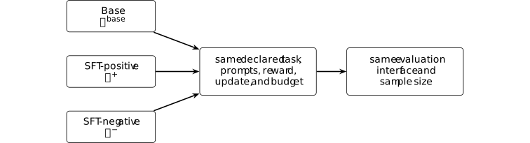
This is the comparison pattern used in [clay2026demystifying, Sections 4.1 and 5.1]. An actual cell still needs its model, task, reward implementation, and numerical record; the diagram is not a claim that all experiments in the paper instantiate one identical grid.

Within a declared model, task, training grid, and evaluation procedure, the three-cell comparison can establish that the measured post-training outcome differs across the source's constructed starting checkpoints. The movie-quote and AIME entries in [clay2026demystifying, Section 5.1, Tables 1--2] are empirical records of that form.

The comparison does not isolate initial target probability from every other SFT-induced weight change, prove that an observed zero has zero support, or establish acquisition of a broader capability. The reported model sets differ across the paper: [clay2026demystifying, Section 4.1] names OLMo 3, Qwen2-7B, Qwen3-1.7B, and Qwen2.5-7B-Instruct, while Table 1 and Appendix G also report Qwen3-8B and Qwen2-1.5B. Each measurement is specific to the model and configuration in its table row.

Fix a starting policy, an evaluation sampling law, and the target predicate of Definition 1.2. Before post-training, draw evaluation records \((X_j,Y_j)_{j=1}^m\). Define the hit indicators and the initial evaluation hit count by

The sampling law determines whether the instances \(X_j\) are fixed, resampled, or stratified. The adjective ``initial'' locates the measurement before the post-training intervention; it does not assert that the samples are independent or that the starting policy is a foundation checkpoint.

For a nonempty initial evaluation sample of size \(m\), the empirical initial success rate is

using the empirical-average convention of Convention [ftip-006Z]. This is a statistic of the declared sample. It is not, without a sampling model and an uncertainty statement, the exact successful-support probability \(p_P(x)\) of Definition [ftip-005U].

The equality \(K_m=0\) says that no target response occurred in one finite sample. Every success probability \(0\leq p<1\) assigns positive probability \((1-p)^m\) to this observation under independent Bernoulli sampling. Thus \(\widehat p_m=0\) does not imply \(p=0\), absence from mathematical support, or impossibility of discovery under a larger budget.

The entries printed as 0.00 percent in [clay2026demystifying, Section 5.1, Tables 1--2] are empirical rates at the stated evaluation sizes. They must not be rewritten as exact support claims.

Let \(m\in \mathbb N_{\geq 1}\). Assume the hit indicators from Definition 2.1 are independent Bernoulli variables with a common success probability \(p\). Then \(K_m\) has the binomial law and

This finite statement follows from the displayed hypotheses. Applying it to a source table requires the additional iid and stationary-success assumptions stated above.

Assume Theorem 2.4 with \(m\in \mathbb N_{\geq 1}\) and fix \(0<\delta <1\). If \(K_m=0\), inversion of the exact zero-count likelihood gives the one-sided upper endpoint

Indeed, \(\Pr _{u_{m,\delta }}(K_m=0)=\delta \), and for every \(p>u_{m,\delta }\) one has \(\Pr _p(K_m=0)<\delta \). Thus the observed zero count excludes probabilities above \(u_{m,\delta }\) at exact level \(\delta \) under the declared iid model.

This is a likelihood inversion derived from the displayed finite setup, not a source theorem and not a support certificate.

Take \(m=128\) and \(\delta =0.05\) in Corollary 2.5. After zero hits, the exact one-sided upper endpoint is

Under the iid Bernoulli model, probabilities above approximately 2.313 percent make a zero count less than five percent likely. The calculation does not turn a recorded \(0/128\) into proof that the true probability is zero, and it does not apply if the 128 evaluations have a different joint sampling law.

Fix an executable sparse-reward rule and let \(r_j^{\mathrm {sp}}\) be the reward returned on rollout \(j\). The first positive sparse-reward time is the extended-valued index

This definition concerns the reward implementation named by an experiment cell. The event \(r_j^{\mathrm {sp}}>0\) coincides with a target-response event only when that equality is part of the declared reward semantics. In particular, a length penalty or partial-credit rule can separate positive reward from exact target match.

Suppose the events \(\{r_j^{\mathrm {sp}}>0\}\) are independent and have a common probability \(q\). For every positive rollout budget \(B\),

This is a specialization proved from the displayed hypotheses. It does not supply independence, stationarity, or the value of \(q\) for a training run, and it does not equate positive proxy reward with task utility.

[clay2026demystifying, Section 5.1, Table 2] reports the following empirical target-answer rates for AIME Problem 4 with Qwen2.5-7B-Instruct and evaluation size \(m=128\). The task asks for the number of integer pairs \((x,y)\in [-100,100]^2\) satisfying \(12x^2-xy-6y^2=0\); the target answer is \(117\).

Every entry in the displayed array is a percentage.

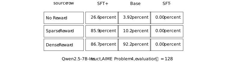
These are source-reported empirical percentages, not exact policy probabilities. ``No Reward'' is retained as the source's row label; the table alone does not define it as a post-training protocol. The three zero entries for SFT-negative are finite observations and remain subject to Remark 2.3. Appendix Figure 5's caption prints a different set of Qwen2.5-7B-Instruct values that duplicates the neighbouring movie-quote caption and is incompatible with Table 2. The displayed percentages are those of Table 2; the caption does not provide a consistent alternative measurement.

[clay2026demystifying, Section 5.2 and Figure 2] report that the Qwen3-1.7B Base movie-quote cell, whose initial empirical match rate is about 0.5 percent, does not optimize under the source's sparse-reward run, whereas its dense-reward run rises toward fifty percent. [clay2026demystifying, Appendix Figure 8] gives final match rates 10.0 percent for sparse reward and 48.8 percent for dense reward. Thus ``failed'' here means failure of the reported sparse run to optimize as intended, not zero final matches.

A plateau is indexed by the model, target, reward implementation, optimizer, sampling process, and budget in its experiment cell. One observed transition therefore does not identify a universal initial-probability threshold for RL learning, support, or capability acquisition.

Let \(\mathcal Y\) be a finite response set and fix a target response \(\tau \in \mathcal Y\). The sparse exact reward is the map \(r_{\rm exact}:\mathcal Y\to \{0,1\}\) defined by

This idealized reward exposes one bit: whether the whole response equals the target. It does not expose a prefix, edit location, or partial milestone. The movie-quote source uses related but textually inconsistent substring and length-penalized rewards; the distinct formulas are compared in Remark 3.2.

Section 4.2 of Demystifying Reinforcement Learning Post-Training of Language Models[clay2026demystifying] displays a substring indicator \(\mathbf 1\{\tau \subseteq y\}\) and says that a length penalty is applied. In Appendix C, \(n\) is the maximum generation length and \(s\) is the number of tokens beyond the target. The appendix first defines the excess-length penalty

and then gives Equation (3):

As printed, Equation (3) assigns zero when \(y=\tau \), because its first branch requires strict excess length. This conflicts with the immediately preceding Appendix-C prose, which assigns base reward one when the target is generated, and it is not the exact-match reward of Definition 3.1. The two printed descriptions therefore specify different reward rules.

Let \(y=y_1\cdots y_m\) and a nonempty target \(\tau =\tau _1\cdots \tau _n\) be finite strings. Their Levenshtein distance is determined by \(D(0,j)=j\), \(D(i,0)=i\), and, for \(i,j>0\),

Set \(L(y,\tau )=\max \{|y|,|\tau |\}\). The edit-distance reward is

The recurrence is Equation (1) in the main text and Equation (4) in Appendix C of Demystifying Reinforcement Learning Post-Training of Language Models[clay2026demystifying]; the normalized reward is its Equation (5). The nonempty-target assumption makes the displayed denominator positive. This reward does not establish that edit similarity is the correct utility for a different task.

The edit reward of Definition 3.3 is not obtained from the binary value in Definition 3.1 by a numerical smoothing operation. It also receives the target string, a character-level edit model, and the ordering of symbols. Two non-target responses that both receive sparse reward zero can therefore receive different edit rewards.

That extra resolution can improve credit assignment, but it changes the feedback channel and its assumptions. The source calls edit distance a dense proxy and reports controlled movie-quote experiments [clay2026demystifying, Sections 4.2 and 5.2]. Neither the formula nor those observations establish that edit proximity is an independent measure of general response quality.

For the source's fixed AIME problem, let

record whether a completed response contains five declared milestones: a valid algebraic setup, correct root relations, correct integer bounds, a correct count for at least one branch, and correct subtraction of the overlap at the origin. With

the milestone process reward is

Appendix D.1 of Demystifying Reinforcement Learning Post-Training of Language Models[clay2026demystifying] gives Equation (6) and the milestone list above. In the experiment, a 32-billion-parameter instruction-tuned model classifies the completed trajectory. The displayed map is therefore richer than a deterministic final-answer verifier, even though it returns one scalar after the rollout.

Appendix D.2 of Demystifying Reinforcement Learning Post-Training of Language Models[clay2026demystifying] supplements \(r_{\rm proc}\) with an extracted-answer override and two penalties. Translating its notation, let \(\tau =117\), \(\tau _{\rm near}=118\), and define

Let \(p_{\rm loop}(y)=-0.3\) when the judge flags a loop without the exact answer, and zero otherwise. Let \(p_{\rm format}(y)=-0.5\) when the response lacks the required boxed delimiter, and zero otherwise. Equations (7)--(8) then give

These clauses assume a reliable milestone judge, parser, near-miss choice, loop flag, and formatting rule. They are part of the feedback definition, not consequences of reinforcement learning. The main text describes ``exponentially increasing'' dense rewards, and Appendix D calls the weights ``exponential scaling.'' The printed vector \((0.05,0.05,0.10,0.15,0.25)\) is neither strictly increasing at every milestone nor a geometric progression. We preserve the exact weights and do not infer an exponential law from that wording.

Let \(\mathcal Y\) be a finite response set and \(r:\mathcal Y\to \mathcal R\) any reward map. Two responses are observationally equivalent under \(r\), written \(y\sim _r y'\), when

Equality makes \(\sim _r\) an equivalence relation. Its quotient \(\mathcal Y/{\sim _r}\) is the finite set of response classes distinguished by the reward alone. This proposed equivalence relation ignores any information in the response that is not returned by \(r\); equal rewards need not imply equal latent utility.

Let \(\mathcal Y\) be finite and let \(r_1:\mathcal Y\to \mathcal R_1\) and \(r_2:\mathcal Y\to \mathcal R_2\). Say that \(r_2\) refines \(r_1\) when

If \(r_2\) refines \(r_1\), then

This finite lemma compares observational partitions only. It does not say that the refined reward is cheaper, more accurate, or better aligned with utility.

Take the target string \(\tau =\texttt {abc}\) and two responses \(y=\texttt {abx}\) and \(y'=\texttt {xyz}\). Both fail exact matching, while their edit distances and normalized edit rewards are

Thus \(y\sim _{r_{\rm exact}}y'\) but \(y\not \sim _{r_{\rm edit}}y'\). The example witnesses a strict separation inside one sparse-reward class. It does not claim that every dense proxy refines every sparse verifier.

One finite response set can be observed through three different maps. The arrows below share a domain; they do not assert that the three codomains form a refinement chain.

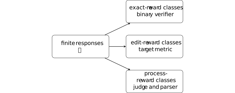
The exact reward forgets every difference among failures. Edit reward can retain character-level proximity, while the source process reward retains a declared milestone vector only after judge, override, and penalty choices. The partition lemma Lemma 3.8 applies to a pair only after its refinement hypothesis has been checked.

A denser reward can distinguish more responses and supply more frequent update signal. It can also require information absent from a sparse verifier. In the controlled source, edit feedback assumes the full target and computes a string metric; process feedback uses a 32-billion-parameter judge, five problem-specific milestones, answer extraction, an enumerated near miss, and loop and format penalties [clay2026demystifying, Appendices C--D].

The richer feedback channel incurs specification, computation, and validation costs. Replacing sparse feedback by dense feedback can alter both the information available to training and the objective being optimized. The resulting comparison is an intervention on feedback resolution, not evidence that one fixed reward was smoothed at zero cost.

Let \(\mathcal X\) be a task-instance set. Write \(\mu _{\rm tr}=\mathcal D_{\rm tr}\) for the training-prompt coordinate of an experiment cell in Definition 1.6. A training prompt law is this probability law on \(\mathcal X\), used to draw instances during a post-training protocol. Let \(\mu _{\rm ev}\) be an independently declared evaluation law on the same set.

An evaluated prompt slice is a measurable set \(C\subseteq \mathcal X\) with \(\mu _{\rm ev}(C)>0\). Its conditional evaluation law is

The training and evaluation laws need not agree. A slice records where an effect is measured; it does not assert that prompts inside the slice are equally difficult or represented equally in pretraining. We specialize the task-law convention of Definition [ftip-001Q].

A prompt configuration is the record

containing the starting artifact, training prompt law, finite prompt-pool size, reward, update algorithm, and training budget. We call two particular records \(\mathsf c_{\rm nar}\) and \(\mathsf c_{\rm brd}\) only when a cited experiment names them narrow and broad.

Section 4.3 and Appendix F of Demystifying Reinforcement Learning Post-Training of Language Models[clay2026demystifying] instantiate these labels in two model-family experiments. The Qwen comparison uses 100 DeepScaleR prompts versus 10,000 WildChat prompts. The OLMo comparison uses 100 math-only prompts versus 10,000 prompts split evenly among mathematics, instruction following, and code. These labels identify the two reported configurations; they do not define a general measure or ordering of prompt breadth.

The records in Definition 4.2 change several coordinates together. The prompt-pool size, domain mixture, and repetition frequency differ. Across the paper's Qwen and OLMo studies, the starting artifact and evaluated tasks also differ.

We therefore use ``narrow'' and ``broad'' as names for the source cells. They do not define a total order on prompt laws, and their comparison does not identify a causal effect of breadth alone. A breadth theorem would need a declared statistic and matched configurations that differ only in that statistic.

Fix an evaluated slice \(C\) from Definition 4.1, and let \(P_0\) and \(P_1\) denote the pre- and post-training protocols whose successful-support probabilities are defined in Definition [ftip-005U]. The slice-conditioned success change is

The evaluation interface, inference budget, and success predicate are held fixed across the two terms. The quantity is an average change on one declared slice. It neither locates the change inside the model nor identifies which training coordinate caused it.

Fix pairwise disjoint evaluated slices \(C_1,\ldots ,C_J\) and a declared degradation threshold \(\kappa >0\). Define the set of materially degraded slices

Degradation is localized relative to this slice family and threshold when \(|\mathcal H_\kappa |=1\). It is distributed when \(|\mathcal H_\kappa |\geq 2\).

These terms depend on the chosen partition, threshold, and evaluation budget. They do not turn a finite benchmark vector into a statement about all capabilities.

Section 5.3 and Appendix F of Demystifying Reinforcement Learning Post-Training of Language Models[clay2026demystifying] supply two OLMo paths; Figure 4 reports their outcomes. Both replace the usual verifiable reward with a random scalar drawn from \(\operatorname {Unif}[0,1]\), but their prompt configurations differ.

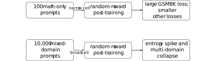
In the narrow SFT-start path, GSM8K accuracy falls from 86 to about 32 by step 400, while the reported MMLU and IFEval changes are much smaller. In the broad path, the source reports an entropy spike near step 400 together with collapse on GSM8K, MMLU, and IFEval. The diagram records that interpretation; it does not isolate prompt breadth from pool size, mixture, or repetition.

Section 5.3 and Figures 3--4 of Demystifying Reinforcement Learning Post-Training of Language Models[clay2026demystifying] report that the Qwen narrow configuration retains higher MATH and AMC Acc@1 than its broad configuration under random reward. The OLMo experiment reports the different evaluation patterns summarized in Example 4.6.

These are finite empirical observations. The random scalar reward removes task alignment from one feedback channel, but it does not hold all other training coordinates fixed. The reported entropy is a named token statistic, not a direct measure of capability or acquisition.

Let two evaluation slices \(C_1,C_2\) have equal mass. A feedback channel returns an independent Bernoulli reward with mean \(1/2\) under either of two post-training protocols. Suppose their fixed-interface success changes are

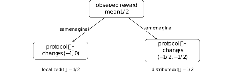
The reward law and its mean are identical, but the slice-level evaluation vectors differ. Hence marginal training reward does not determine whether damage is localized or distributed. This is a finite counterexample, not a claim about the mechanism in the source experiment.

The source cells motivate tests of starting-policy coverage, feedback resolution, and prompt-conditioned damage. They do not establish that dense reward creates mathematical support, that zero sampled hits imply zero probability, or that random reward has one model-independent effect.

Separating the effects of coverage, feedback resolution, and prompt breadth requires stronger controls. One comparison fixes prompt laws and varies only the feedback sigma-algebra. Another fixes feedback and evaluation while varying one starting-policy coordinate. Confidence regions for the complete vector of slice-conditioned changes would quantify effects that an aggregate score can hide.

The reported observations remain conditional on their experimental configurations. They do not establish general results about capability acquisition, elicitation, or the optimal allocation of post-training compute.