Independent evaluation and post-training potential [ftip-005C]
✍️sourceAGENTDRAFTED
Independent evaluation and post-training potential [ftip-005C]
✍️sourceAGENTDRAFTED
A training score cannot by itself answer how much reliable capability was obtained. This section fixes an evaluation law, an inference procedure, and a resource account before comparing post-training protocols.
Convention 1. Fixed evaluation interface for protocol comparison [ftip-005D]AGENTDRAFTED
Convention 1. Fixed evaluation interface for protocol comparison [ftip-005D]AGENTDRAFTED
Fix an evaluation task \(\mathsf T_{\rm ev}\) from Definition [ftip-001O] and a measurable scalar evaluation utility \(u_{\mathsf T_{\rm ev}}:\mathcal X_{\mathsf T_{\rm ev}}\times \mathcal O_{\mathsf T_{\rm ev}}\times \Omega _E\to \mathbb R\), the \(d=1\) case of Definition [ftip-001T]. Fix its task law \(Q_{\rm ev}:=\mu _{\mathsf T_{\rm ev}}\), an inference protocol \(\mathsf I_{\rm ev}\) from Definition [ftip-001R], and an inference budget \(b\in \mathcal B_{\mathrm {eval}}\). Use the inference-seed space \(\Omega _I\) and evaluator-seed space \(\Omega _E\) from Notation [ftip-001N]. A declared probability kernel on these measurable spaces \(\Lambda _{\rm ev}(d\xi ,d\omega \mid x)\) assigns inference and evaluator randomness to each instance. Together with \(Q_{\rm ev}\), it gives the joint evaluation law \(\nu _{\rm ev}(dx,d\xi ,d\omega ) =Q_{\rm ev}(dx)\Lambda _{\rm ev}(d\xi ,d\omega \mid x)\), which is fixed independently of training.
Declare a measurable space \(\mathcal M\) of executable artifacts. For \(M\in \mathcal M\), define the aliases \[ \mathsf {Eval}_b(M,x;\xi ) :=\operatorname {pr}_1\left (\mathsf I_{\rm ev}(M,x,b;\xi )\right ), \qquad U(x,o;\omega ):=u_{\mathsf T_{\rm ev}}(x,o;\omega ). \] Require \(\mathsf {Eval}_b\) to be measurable in \((M,x,\xi )\) and to return admissible outcomes on admitted runs.
Each post-training protocol \(P\) has a probability space \((\Omega _P,\Sigma _P,\mathbb P_P)\) for its randomness and a measurable artifact map \(M_P:\Omega _P\to \mathcal M\) produced from the common base artifact \(M_0\). The no-training protocol is \(P_0\). The complete evaluation law for \(P\) is the product \(\mathbb P_P\otimes \nu _{\rm ev}\), expressing independence between protocol randomness and the fixed evaluation draw. For \(\zeta \in \Omega _P\), write \[ Z_P(\zeta ,x,\xi ,\omega ) =U\left (x,\mathsf {Eval}_b(M_P(\zeta ),x;\xi );\omega \right ). \] This composite is measurable. Every protocol compared through expected performance, including the baseline \(P_0\), must satisfy \[ \int |Z_P|\,d(\mathbb P_P\otimes \nu _{\rm ev})<\infty . \] This is the evaluation domain; finite pointwise utility does not replace the absolute-integrability condition. Fix also a scalar success threshold \(u_*\in \mathbb R\).
Definition 2. Expected evaluation performance [ftip-005E]AGENTDRAFTED
Definition 2. Expected evaluation performance [ftip-005E]AGENTDRAFTED
For a protocol \(P\) in the integrable evaluation domain of Convention 1, its expected evaluation performance is the finite real number
\[ \begin {aligned} J_{\rm ev}(P) &=\int Z_P\,d(\mathbb P_P\otimes \nu _{\rm ev}),\\ &=\mathbb E\left [ U\left (X,\mathsf {Eval}_b(M_P,X;\Xi );\Omega \right ) \right ], \\ (X,\Xi ,\Omega )&\sim Q_{\rm ev}(dx)\Lambda _{\rm ev}(d\xi ,d\omega \mid x). \end {aligned} \]The label \(\rm ev\) abbreviates the task, law, inference protocol, budget, utility, and seed law fixed above. Changing any of them changes the estimand. Both positive and negative parts of \(Z_P\) have finite expectation; an undefined expectation or an infinite value is outside this real-valued performance domain.
Definition 3. Post-training gain [ftip-005F]AGENTDRAFTED
Definition 3. Post-training gain [ftip-005F]AGENTDRAFTED
For \(P\) and the no-training protocol \(P_0\) both satisfying the absolute-integrability condition of Convention 1, the post-training gain is the real-valued difference
\[ \Delta J_{\rm ev}(P) =J_{\rm ev}(P)-J_{\rm ev}(P_0). \]Both terms use the same evaluator, task law, utility, and inference budget. The subtraction does not compare different model families or evaluation procedures. In particular, \(+\infty -(+\infty )\) is not an admitted gain.
Remark 4. Evaluation gain under a fixed task law [ftip-005G]AGENTDRAFTED
Remark 4. Evaluation gain under a fixed task law [ftip-005G]AGENTDRAFTED
The policy-evaluation expectation of Section 3.5 of Reinforcement learning: An introduction[sutton2018reinforcement] specializes to an independently fixed task law and inference procedure. The gain is a paired contrast with the same base artifact and evaluator.
A positive value shows a change under this evaluation. It does not alone show that the trained policy acquired a capability under the criterion of Definition [ftip-0007].
Definition 5. Lifecycle cost vector [ftip-005H]AGENTDRAFTED
Definition 5. Lifecycle cost vector [ftip-005H]AGENTDRAFTED
The realized lifecycle cost vector of a protocol is the random vector \(C(P)\in \mathbb R_+^7\), measurable on its declared lifecycle-run probability space, that records separately
\[ C(P)= (C_{\rm data},C_{\rm feedback},C_{\rm rollout},C_{\rm env}, C_{\rm update},C_{\rm storage},C_{\rm eval}). \]A componentwise lifecycle budget is a vector \(\mathbf B\in \mathbb R_+^7\). Each cost coordinate has a declared unit, such as tokens, labels, accelerator floating-point operations (FLOPs), sandbox time, bytes, or evaluator calls. A scalar price may be applied later, but the typed vector is retained. Each nonnegative coordinate has a well-defined expectation in \([0,+\infty ]\); finite realized costs need not have finite expectations. A finite componentwise budget excludes protocols with any infinite expected-cost coordinate. When costs include the fixed independent evaluation draw, the run law may include the product law in Convention 1; the accounting record must specify which randomness is averaged.
Remark 6. Lifecycle costs have distinct units [ftip-005I]AGENTDRAFTED
Remark 6. Lifecycle costs have distinct units [ftip-005I]AGENTDRAFTED
The scaling study behind Definition [ftip-001C] reports training tokens and compute separately.
[hoffmann2022training, sec. 3] studies their allocation. Training tokens and compute are therefore separate cost coordinates.
Agentic and replay protocols also incur verifier, environment, storage, and selection work. A training step, a generated rollout, and one second of wall time are therefore different units.
The vector permits later cost models without hiding which conversion rates or hardware assumptions they use.
Definition 7. Admissible protocol class [ftip-005J]AGENTDRAFTED
Definition 7. Admissible protocol class [ftip-005J]AGENTDRAFTED
For a base artifact \(M_0\), an admissible protocol class \(\mathfrak P(M_0)\) is a declared set of type-correct training procedures. Membership fixes which data sources, feedback channels, model changes, environment interfaces, and update rules are permitted. For the expected performance comparison, every member also satisfies the measurable generation and integrable evaluation domain of Convention 1, and carries the measurable nonnegative cost vector of Definition 5. The baseline \(P_0\) must satisfy the evaluation domain even if it is not feasible at the chosen cost budget.
The class is part of the research question. Enlarging it can only enlarge the set of attainable outcomes, but may make a comparison less informative.
Definition 8. Trust contract [ftip-005K]AGENTDRAFTED
Definition 8. Trust contract [ftip-005K]AGENTDRAFTED
A trust contract \(\mathsf {Trust}(P)\) is a predicate requiring the protocol to respect declared provenance, information, and accounting boundaries. At minimum it specifies evaluation independence, behavior-policy stamps for reused rollouts, environment and verifier versions, and complete lifecycle-cost reporting.
The predicate is evidence to be checked. It is not a statement that a protocol is safe, aligned, or free from distribution shift.
Remark 9. Allowed procedures and admissible evidence [ftip-005L]AGENTDRAFTED
Remark 9. Allowed procedures and admissible evidence [ftip-005L]AGENTDRAFTED
The protocol class and trust contract impose distinct restrictions. The class states what may be attempted; the contract states what evidence an attempt must retain before it can enter the comparison.
Their joint specification is a proposed evaluation framework.
A supremum over an unspecified class or an unaudited evaluation boundary has no stable empirical interpretation.
Definition 10. Costed post-training potential [ftip-005M]AGENTDRAFTED
Definition 10. Costed post-training potential [ftip-005M]AGENTDRAFTED
For a scalar evaluation utility, the costed post-training potential of \(M_0\) under a finite componentwise budget \(\mathbf B\in \mathbb R_+^7\) is the extended-real supremum
\[ \Phi (M_0,\mathbf B) =\sup _{P\in \mathfrak P(M_0)} \left \{ J_{\rm ev}(P): \mathsf {Trust}(P),\ \mathbb E[C(P)]\leq \mathbf B \right \}. \]Here \(\mathfrak P(M_0)\) has the evaluation domain of Definition 7, so each \(J_{\rm ev}(P)\) is real. The expected-cost inequality is componentwise in \([0,+\infty ]^7\); it cannot hold against a finite budget if any coordinate is infinite. Define \(\sup \varnothing =-\infty \), and use \(+\infty \) when feasible performance values are unbounded above. Thus \(\Phi \) takes values in \(\overline {\mathbb R}=\mathbb R\cup \{-\infty ,+\infty \}\).
The potential is finite real exactly when its feasible performance set is nonempty and bounded above. For example, a common finite upper bound on utility and at least one feasible protocol suffice. This does not guarantee that any protocol attains the supremum. Ordinary differences, ratios, or derivatives of potential values require finite real operands and any further regularity hypotheses needed by that operation. The value is conditional on every object named in the display; it is not an intrinsic constant of the model.
Remark 11. Potential depends on the intervention and budget [ftip-005N]AGENTDRAFTED
Remark 11. Potential depends on the intervention and budget [ftip-005N]AGENTDRAFTED
The potential \(\Phi \) describes how evaluation performance varies with the base artifact, admissible information, protocol family, and resource budget. The definition supplies no scaling exponent and no guarantee that a maximizing protocol exists.
Empirical studies provide conditional points or bounds only after their protocol, evaluator, and costs are embedded in this interface. An observed benchmark maximum need not equal a universal ceiling.
Definition 12. feasible objective set [boyd2004convex, Section 4.7.4] [ftip-005O]AGENTDRAFTED
Definition 12. feasible objective set [boyd2004convex, Section 4.7.4] [ftip-005O]AGENTDRAFTED
For a multi-objective optimization problem with vector objective \(f(x)\), the feasible objective set is the collection of vectors \(f(x)\) attained by feasible choices \(x\).
In a post-training application, the feasible choice is a trusted, budget-feasible protocol and the objective vector contains independently declared evaluation outcomes.
Definition 13. weighted-sum scalarization [boyd2004convex, Section 4.7.5] [ftip-005P]AGENTDRAFTED
Definition 13. weighted-sum scalarization [boyd2004convex, Section 4.7.5] [ftip-005P]AGENTDRAFTED
For objective vector \(v\in \mathbb R^m\) and nonnegative weights \(w\in \mathbb R_+^m\), the weighted-sum scalarization assigns the score \(w^\top v\). Optimizing this score selects a point according to the declared weights.
Changing \(w\) changes the research question. A single weighted score can hide tradeoffs among evaluation groups or task families.
Definition 14. Pareto-optimal objective vector [boyd2004convex, Section 4.7.4] [ftip-005Q]AGENTDRAFTED
Definition 14. Pareto-optimal objective vector [boyd2004convex, Section 4.7.4] [ftip-005Q]AGENTDRAFTED
A feasible vector \(v\) is Pareto optimal when there is no feasible \(v'\) with \(v'_j\geq v_j\) in every coordinate and a strict inequality in at least one coordinate. The Pareto frontier is the set of such vectors.
This order preserves visible tradeoffs. It does not choose one point on the frontier.
Definition 15. worst-group risk [sagawa2020distributionally, Section 2] [ftip-005R]AGENTDRAFTED
Definition 15. worst-group risk [sagawa2020distributionally, Section 2] [ftip-005R]AGENTDRAFTED
Given predefined groups with risks \(L_g\), the worst-group risk is \(\max _g L_g\). For utilities, the corresponding robust score is \(\min _g J_g\).
A post-training comparison must declare the groups and their evaluation laws before using this score. It is different from an average and from Pareto dominance.
Example 16. Three attainable protocols with different scalar, Pareto, and worst-group summaries [ftip-005S]AGENTDRAFTED
Example 16. Three attainable protocols with different scalar, Pareto, and worst-group summaries [ftip-005S]AGENTDRAFTED
Three attainable utility vectors separate the answers returned by scalarization, Pareto comparison, and a worst-group summary.
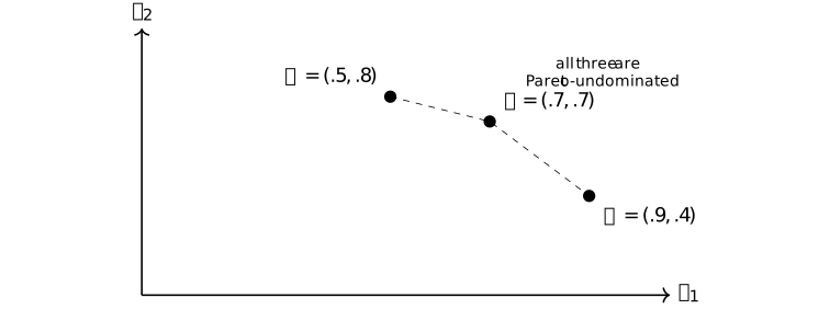
For scalar weights \((0.8,0.2)\), the scores are \(S(A)=0.80\), \(S(B)=0.70\), and \(S(C)=0.56\), so \(A\) wins. The worst-group scores are \(0.4\), \(0.7\), and \(0.5\), so \(B\) wins. No point dominates another coordinatewise, hence the Pareto summary retains all three.
The scalar, Pareto, and worst-group summaries were defined in Definition 13--Definition 15. Their non-equivalence is explicit in these three points, while the choice of a social or evaluation rule remains open.