Decoder-only Transformer architecture [ftip-000K]
✍️sourceAGENTDRAFTED
Decoder-only Transformer architecture [ftip-000K]
✍️sourceAGENTDRAFTED
The continuation law in Definition [ftip-000I] specifies what probabilities a language model exposes. A decoder-only Transformer specifies how a sequence of token identifiers is transformed into those probabilities. This section introduces one component at a time, with dimensions fixed before the component formulas are used.
Notation 1. Tensor dimensions, positions, heads, and layers [ftip-000L]AGENTDRAFTED
Notation 1. Tensor dimensions, positions, heads, and layers [ftip-000L]AGENTDRAFTED
Let \(T\) be the maximum token positions processed together, \(d\) the residual-stream width, \(d_{\mathrm {ff}}\) a feed-forward hidden width, \(H\) the number of attention heads, \(d_h\) the query-key width of one head, and \(L\) the number of decoder layers. Positions are indexed by \(t,s\in \{1,\ldots ,T\}\), heads by \(h\in \{1,\ldots ,H\}\), and layers by \(\ell \in \{1,\ldots ,L\}\).
A batch of \(B\) hidden-state sequences is a tensor in \(\mathbb R^{B\times T\times d}\). When the batch coordinate is irrelevant, write \(X\in \mathbb R^{T\times d}\) and let \(X_t\in \mathbb R^d\) denote its row at position \(t\). Matrix products act on the final coordinate.
Definition 2. Token embedding [vaswani2017attention, sec. 3.4, Embeddings and Softmax] [ftip-000M]AGENTDRAFTED
Definition 2. Token embedding [vaswani2017attention, sec. 3.4, Embeddings and Softmax] [ftip-000M]AGENTDRAFTED
Let \(\mathcal V\) be the vocabulary of Definition [ftip-000D] and \(d\) the residual width of Notation 1. A token embedding matrix is a learned matrix \(E\in \mathbb R^{|\mathcal V|\times d}\). The hidden vector assigned to token \(a\in \mathcal V\) is the row \(E_a\in \mathbb R^d\).
For a sequence \(x_{1:n}\), embedding lookup produces the matrix \(X^{\mathrm {tok}}\in \mathbb R^{n\times d}\) with row \(X^{\mathrm {tok}}_t=E_{x_t}\). This operation maps token identifiers to vectors; it does not yet encode their positions.
Definition 3. Embedding-stage positional transformation [ftip-000N]AGENTDRAFTED
Definition 3. Embedding-stage positional transformation [ftip-000N]AGENTDRAFTED
Using the dimensions of Notation 1, an embedding-stage positional transformation is a specified family of position-dependent transformations \(r_t:\mathbb R^d\to \mathbb R^d\), one for each \(t\in \{1,\ldots ,T\}\). Applied after the token embedding of Definition 2, it produces the initial hidden vector \[ X^{(0)}_t=r_t(E_{x_t}). \] The family \((r_t)_{t=1}^T\) is part of the architecture, even when it has no learned parameters.
Remark 4. Where positional information enters [ftip-000O]AGENTDRAFTED
Remark 4. Where positional information enters [ftip-000O]AGENTDRAFTED
Definition 3 covers only mechanisms acting on the hidden vector at the embedding stage. The original Transformer adds a fixed or learned vector \(p_t\) to the token embedding, so \(r_t(z)=z+p_t\); see [vaswani2017attention, §3.5].
Relative-bias methods instead alter an attention score as a function of the displacement \(t-s\). ALiBi gives one such construction in [press2021train, §3].
Rotary position embedding applies position-indexed rotations to queries and keys rather than adding a vector to the residual stream; see RoFormer, Section 3.2, equations (14)--(16) [⧉]. These mechanisms are not interchangeable choices of one tensor: they act at different points in the computation, so a model specification must name the mechanism and placement.
Definition 5. Query, key, and value projections [vaswani2017attention, sec. 3.2.1] [ftip-000P]AGENTDRAFTED
Definition 5. Query, key, and value projections [vaswani2017attention, sec. 3.2.1] [ftip-000P]AGENTDRAFTED
Let \(X\in \mathbb R^{T\times d}\) use the notation of Notation 1. For attention head \(h\), choose learned matrices \[ W_h^Q,W_h^K\in \mathbb R^{d\times d_h}, \qquad W_h^V\in \mathbb R^{d\times d_v}, \] where \(d_v\) is the value width of one head. The query, key, and value matrices are \[ Q_h=XW_h^Q,\qquad K_h=XW_h^K,\qquad V_h=XW_h^V. \] Their rows associate a query, key, and value vector with each token position.
Definition 6. Scaled dot-product attention [vaswani2017attention, sec. 3.2.1, equation (1)] [ftip-000Q]AGENTDRAFTED
Definition 6. Scaled dot-product attention [vaswani2017attention, sec. 3.2.1, equation (1)] [ftip-000Q]AGENTDRAFTED
Using the head widths in Definition 5, let \(T_q,T_k\geq 1\) be query and key-value sequence lengths. For \(Q\in \mathbb R^{T_q\times d_h}\), \(K\in \mathbb R^{T_k\times d_h}\), and \(V\in \mathbb R^{T_k\times d_v}\), scaled dot-product attention is \[ \operatorname {Att}(Q,K,V) =\operatorname {softmax}\left (\frac {QK^{\mathsf T}}{\sqrt {d_h}}\right )V. \] The softmax is applied across each row of the \(T_q\times T_k\) score matrix, so every output row is a convex combination of the value rows.
Example 7. A two-token attention calculation [ftip-000R]AGENTDRAFTED
Example 7. A two-token attention calculation [ftip-000R]AGENTDRAFTED
A scalar attention head on two positions makes the masked softmax and its resulting value average explicit.

Take head width \(d_h=1\), so the scale \(1/\sqrt {d_h}\) is one. At position two both keys are causally available. Therefore \[ \operatorname {softmax}(0,\log 3) =\frac {(1,3)}{1+3} =\left (\tfrac 14,\tfrac 34\right ), \qquad z_2=\tfrac 14\cdot 2+\tfrac 34\cdot 6=5. \]
Substitution into the scaled dot-product attention of Definition 6 produces the displayed value. Projection matrices, multiple heads, normalization, and residual connections remain outside this scalar calculation; it represents only one attention operation.
Definition 8. Causal attention mask [vaswani2017attention, sec. 3.2.3] [ftip-000S]AGENTDRAFTED
Definition 8. Causal attention mask [vaswani2017attention, sec. 3.2.3] [ftip-000S]AGENTDRAFTED
For a length-\(T\) sequence, the causal attention mask is the matrix \(M\in (\mathbb R\cup \{-\infty \})^{T\times T}\) with \[ M_{ts}= \begin {cases} 0,&s\leq t,\\ -\infty ,&s>t. \end {cases} \] Masked self-attention replaces the score matrix in Definition 6 by \(QK^{\mathsf T}/\sqrt {d_h}+M\). Consequently, the output at position \(t\) has zero attention weight on every later position \(s>t\).
Example 9. A length-four causal mask [ftip-000T]AGENTDRAFTED
Example 9. A length-four causal mask [ftip-000T]AGENTDRAFTED
For four positions, a causal mask admits the current and earlier keys and excludes every future key.

Rows index querying positions and columns index key positions. In row three, the first three entries remain available and the fourth receives \(-\infty \); after softmax the fourth token therefore contributes exactly zero.
The construction is the autoregressive mask of [vaswani2017attention, Section 3.2.3]. It enforces a dependency restriction. Effective use of the available earlier positions is a separate model property.
Definition 10. Multi-head self-attention [vaswani2017attention, sec. 3.2.2] [ftip-000U]AGENTDRAFTED
Definition 10. Multi-head self-attention [vaswani2017attention, sec. 3.2.2] [ftip-000U]AGENTDRAFTED
For each head \(h\in \{1,\ldots ,H\}\), form \(Q_h,K_h,V_h\) as in Definition 5 from the same input \(X\), and apply the masked attention of Definition 8: \[ Z_h=\operatorname {softmax}\left ( \frac {Q_hK_h^{\mathsf T}}{\sqrt {d_h}}+M \right )V_h. \] With \(W^O\in \mathbb R^{H d_v\times d}\), multi-head self-attention is \[ \operatorname {MHA}(X) =\operatorname {Concat}(Z_1,\ldots ,Z_H)W^O. \] It returns one width-\(d\) vector at every input position.
Remark 11. Multi-head, grouped-query, and compressed-attention variants [ftip-000V]AGENTDRAFTED
Remark 11. Multi-head, grouped-query, and compressed-attention variants [ftip-000V]AGENTDRAFTED
The multi-head construction in Definition 10 stores a key and value projection per query head. Grouped-query attention instead partitions query heads into groups that share key and value heads; see Ainslie et al., Section 2 [⧉]. This changes parameter and cache shapes while preserving the query-key-value semantics.
Multi-head latent attention first compresses key-value information through a lower-dimensional latent representation and reconstructs head-specific quantities; see DeepSeek-V2, Section 2.1 [⧉]. DeepSeek-V3, Section 2.1, records a later use of that architecture [⧉]. These architectural differences do not establish that their post-training effects equal those of ordinary multi-head attention.
Definition 12. Positionwise feed-forward sublayer [vaswani2017attention, sec. 3.3, equation (2)] [ftip-000W]AGENTDRAFTED
Definition 12. Positionwise feed-forward sublayer [vaswani2017attention, sec. 3.3, equation (2)] [ftip-000W]AGENTDRAFTED
With widths \(d\) and \(d_{\mathrm {ff}}\) from Notation 1, a positionwise feed-forward sublayer is a map \(F:\mathbb R^d\to \mathbb R^d\) of the form \[ F(z)=\phi (zW_1+b_1)W_2+b_2, \] where \(W_1\in \mathbb R^{d\times d_{\mathrm {ff}}}\), \(W_2\in \mathbb R^{d_{\mathrm {ff}}\times d}\), the vectors \(b_1,b_2\) have the corresponding widths, and \(\phi \) is applied coordinatewise. The same map is applied independently at each token position.
Definition 13. Sparse mixture-of-experts routing [ftip-000X]AGENTDRAFTED
Definition 13. Sparse mixture-of-experts routing [ftip-000X]AGENTDRAFTED
Let \(J\geq 1\) and \(1\leq k\leq J\). Let \(F_1,\ldots ,F_J:\mathbb R^d\to \mathbb R^d\) be feed-forward experts and let \(g:\mathbb R^d\to \mathbb R^J\) be a router. For a hidden vector \(z\), let \(S_k(z)\) be the indices of the \(k\) largest coordinates of \(g(z)\), breaking equal scores by a fixed total order on expert indices. A sparse mixture-of-experts layer returns \[ F_{\mathrm {MoE}}(z) =\sum _{j\in S_k(z)}\alpha _j(z)F_j(z), \qquad \alpha _j(z)= \frac {\exp g_j(z)}{\sum _{i\in S_k(z)}\exp g_i(z)}. \] Only the selected experts are evaluated for that token.
Remark 14. Dense and routed feed-forward computation [ftip-000Y]AGENTDRAFTED
Remark 14. Dense and routed feed-forward computation [ftip-000Y]AGENTDRAFTED
The dense sublayer in Definition 12 evaluates one learned map for every token. The sparsely gated construction of Shazeer et al., Section 2, selects among multiple experts and introduces an additional routing and load-balancing problem [⧉]. The top-\(k\) selection rule is described in Definition 13.
Parameter count, active parameter count, and executed operations therefore need not agree. A post-training comparison involving routed models must state which quantity is held fixed and whether the router itself is updated.
Example 15. Top-k expert routing and its DeepSeek counterpart [ftip-000Z]AGENTDRAFTED
Example 15. Top-k expert routing and its DeepSeek counterpart [ftip-000Z]AGENTDRAFTED
A routed mixture-of-experts layer uses router scores to activate only a declared subset of routed experts, then combines their outputs with any shared expert path.

The revision-pinned configuration [⧉] declares \(256\) routed experts, \(6\) experts selected per token, and one shared expert. This instantiates the selection interface while leaving the artifact's router scores, load-balancing mechanism, and expert outputs unspecified.
Definition 16. Residual connection [vaswani2017attention, sec. 3.1] [ftip-0010]AGENTDRAFTED
Definition 16. Residual connection [vaswani2017attention, sec. 3.1] [ftip-0010]AGENTDRAFTED
Using the sequence and residual dimensions of Notation 1, let \(F:\mathbb R^{T\times d}\to \mathbb R^{T\times d}\) be a sublayer whose input and output have the same shape. A residual connection forms \[ R_F(X)=X+F(X). \] The addition is coordinatewise. Shape equality is part of the construction; the residual path is not a concatenation of features.
Definition 17. Layer normalization [ba2016layer, sec. 3] [ftip-0011]AGENTDRAFTED
Definition 17. Layer normalization [ba2016layer, sec. 3] [ftip-0011]AGENTDRAFTED
For the residual width \(d\) of Notation 1, a declared numerical stabilizer \(\varepsilon _{\mathrm {LN}}>0\), and \(z=(z_1,\ldots ,z_d)\in \mathbb R^d\), define \(\mu (z)=d^{-1}\sum _i z_i\) and \(\sigma ^2(z)=d^{-1}\sum _i(z_i-\mu (z))^2\). With learned vectors \(\gamma ,\beta \in \mathbb R^d\), layer normalization is \[ \operatorname {LN}(z) =\gamma \odot \frac {z-\mu (z)\mathbf 1} {\sqrt {\sigma ^2(z)+\varepsilon _{\mathrm {LN}}}}+\beta . \] It is applied independently to the hidden vector at each token position. The declared stabilizer makes the numerical operator total on \(\mathbb R^d\); the unstabilized expression is recovered where \(\sigma ^2(z)>0\) by setting \(\varepsilon _{\mathrm {LN}}=0\).
Definition 18. Normalization placement [ftip-006E]AGENTDRAFTED
Definition 18. Normalization placement [ftip-006E]AGENTDRAFTED
For a residual stream \(X\), a sublayer \(F\), and a normalization operator \(N\), post-normalization applies \(N(X+F(X))\). In pre-normalization, the sublayer receives a normalized input and the residual update is \(X+F(N(X))\).
Placement is an architecture coordinate, separate from the formula for \(N\). Every decoder block must state which residual branches use which placement.
Definition 19. Root mean square layer normalization [zhang2019root, Section 4, equation (4)] [ftip-006F]AGENTDRAFTED
Definition 19. Root mean square layer normalization [zhang2019root, Section 4, equation (4)] [ftip-006F]AGENTDRAFTED
For \(z\in \mathbb R^d\), learned scale \(\gamma \in \mathbb R^d\), and a declared numerical stabilizer \(\varepsilon _{\mathrm {RMS}}>0\), root mean square layer normalization is
\[ \operatorname {RMSNorm}(z) =\gamma \odot \frac {z}{\sqrt {d^{-1}\sum _{i=1}^{d}z_i^2+ \varepsilon _{\mathrm {RMS}}}}. \]Unlike layer normalization in Definition 17, this operator does not subtract the coordinate mean. The declared stabilizer makes it total at the zero vector; setting the stabilizer to zero recovers the source expression on nonzero inputs.
Remark 20. Normalization operator and placement are separate choices [ftip-006G]AGENTDRAFTED
Remark 20. Normalization operator and placement are separate choices [ftip-006G]AGENTDRAFTED
Ba et al. define layer normalization in [ba2016layer, Section 3]. The original Transformer applies it after residual addition in [vaswani2017attention, Section 3.1]. Xiong et al. distinguish post-normalized and pre-normalized Transformers in [xiong2020layer, Section 3.3]. Either the normalization operator or its placement can change while the other is held fixed.
A later stability statement must therefore name both choices. A result about the normalization formula alone does not determine the residual path.
Definition 21. Decoder-only Transformer language model [phuong2022formal, sec. 6, Decoder-only transformers] [ftip-0012]AGENTDRAFTED
Definition 21. Decoder-only Transformer language model [phuong2022formal, sec. 6, Decoder-only transformers] [ftip-0012]AGENTDRAFTED
A decoder-only Transformer language model consists of:
- the token interface in Definition [ftip-000E];
- an initial representation from Definition 2 and Definition 3;
- a stack of \(L\) causal decoder layers built from the attention, feed-forward, residual, and normalization constructions in Definition 8--Definition 17; and
- an output map from the final hidden vector to token logits.
If the final hidden vector at position \(t\) is \(h_t\in \mathbb R^d\), an output matrix \(W_U\in \mathbb R^{|\mathcal V|\times d}\) and bias \(b_U\in \mathbb R^{|\mathcal V|}\) give logits \(z_t=W_Uh_t+b_U\). The softmax \[ \pi _\theta (a\mid x_{1:t}) =\frac {\exp (z_{t,a})} {\sum _{v\in \mathcal V}\exp (z_{t,v})} \] realizes the conditional next-token law of Definition [ftip-000H]. The parameter tuple \(\theta \) contains every learned tensor named by this architecture.
Example 22. Decoder-only dataflow and a DeepSeek V4-Flash provenance overlay [ftip-0013]AGENTDRAFTED
Example 22. Decoder-only dataflow and a DeepSeek V4-Flash provenance overlay [ftip-0013]AGENTDRAFTED
A decoder pipeline maps token identifiers through hidden states to logits; the released model instance and family report provide different evidence about that pipeline.
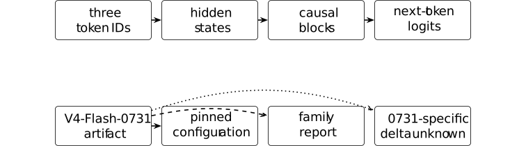
The pinned configuration [⧉] declares 43 layers, hidden width 4096, 64 attention heads, and one key--value head. Section 2 of the family report [⧉] describes the preview architecture. Neither source identifies a complete 0731-specific architecture or training delta. The diagram records the interface, not a small copy of the released model.