Notes on formalized theoretical intelligence potential [ftip-0001]
- August 27, 2026
- Utensil Song
Notes on formalized theoretical intelligence potential [ftip-0001]
- August 27, 2026
- Utensil Song
Formalized Theoretical Intelligence Potential (FTIP) studies how much reliable capability post-training and agent procedures can obtain from a specified pretrained model, and how that capability depends on information, feedback, computation and evaluation. The question is comparative: what improves, through which mechanism, at what cost, and on which tasks? It concerns behavior under specified conditions, rather than an intrinsic intelligence number assigned to a model.
Post-training studies how demonstrations, preferences, rewards and interaction change a model's policy. Fine-tuning, direct preference optimization, and reinforcement learning with human or verifiable feedback differ in their objectives, feedback and update procedures. Agent systems add another source of change: tool use, search, persistent state and retained context can alter behavior even with fixed model weights. Their computation, failure modes and reliability are part of the capability being studied.
Evaluation and finite limits ask which improvements survive independent testing, what transfers to other task laws, and what follows from assumptions about sampling, support, feedback and proxy error. Architecture and optimization ask how the model's computation, parameterization and optimizer affect achievable capability and resource tradeoffs. Its mechanism map asks which bottleneck a design changes and what evidence would demonstrate that change, without ranking architectures. Matched comparisons connect these questions without identifying a higher training reward, a successful rollout and a transferable capability as the same outcome.
Conceptual discovery across generations extends the study to successive learned artifacts, reusable representations, curricula and contributions from independently developed researchers. It asks when a system can discover a method and acquire the ability to use it on fresh problems, with development and learning costs included. Mathematical research supplies concrete settings for that question; the proposed discovery-cost separation remains open.
Civilization and economic reproduction ask how learning resources arise from productive capacity, finance and the renewal of knowledge. Economic development can constrain a campaign or expand its future resources. The chapter proves conditional bounds for specified models and studies reliable contributions and shared preparation costs, alongside alternative models that sustain continued learning. These results make the budget part of the mathematical question; the general discovery lower bound remains open.
The shared model, task and evaluation interfaces support these different lines of inquiry. The notes combine published empirical observations, specified mechanisms, finite mathematical results and open research questions. Each result has its own assumptions and scope; a capability claim depends on the starting artifact, the intervention, independent evaluation and resource bounds.
Remark. How to read these notes [ftip-00NW]AGENTDRAFTED
Remark. How to read these notes [ftip-00NW]AGENTDRAFTED
The seven chapters connect learning mechanisms, computational constraints, agent reliability, evaluation, capability growth and economic conditions. The diagram shows their main logical relationships. Solid arrows indicate concepts used by another analysis. The dashed branch supplies architecture-specific detail for comparisons involving a particular model implementation or optimizer. Within that branch, the mechanism map identifies which capability bottleneck changes and what evidence would show the change; the second dashed edge marks its possible consequences for representations and discovery across model generations.
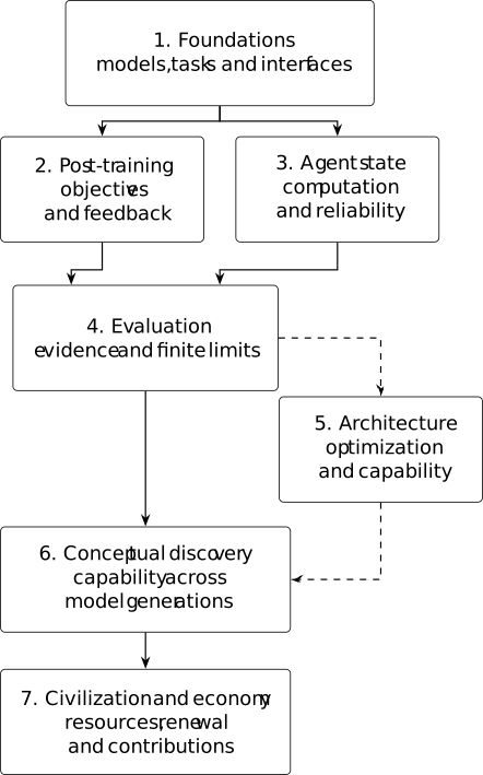
Post-training and agent state are complementary sources of capability change: one changes learned parameters, while the other manages interaction, computation and retained artifacts. Evaluation studies the evidence for those changes and their limits. Architecture analysis connects the comparison to the model's computation and optimization. The lineage analysis extends it to discovery and learning across generations. Economic analysis then asks how productive capacity, knowledge renewal and financing make the required resources available, and how learning changes those conditions.
- Foundations and interfaces introduces capability claims, token probabilities, pretraining, tasks and environments. These interfaces allow the later analysis to specify a model without requiring a particular neural architecture.
- Post-training, alignment, and feedback develops fine-tuning, preference learning, RLHF, DPO, RLVR and agentic training, with concrete objectives, feedback mechanisms and update procedures.
- Agent state, computation, and reliability studies persistent state, retained context, recursive execution, failure modes and reliability. It separates changes to agent behavior from changes to model weights while examining their interaction.
- Evaluation, evidence, and finite limits fixes the comparison law and costs, studies transport to other evaluations, and develops finite results about discovery, support, feedback and proxy error. Its closing synthesis collects the consequences and counterexamples.
- Architecture-conditioned potential and computation begins with a decoder-only Transformer, then uses the mechanism-family map to ask which capability bottleneck a design changes. Its optimization-geometry and matched-compute sections use the evaluation framework to make implementation-specific claims. The core panel is the default comparison path; the adjunct panel supplies optional objective, temporal-dynamics and function-space lenses.
- Conceptual discovery across model generations studies discovery and learning across successive artifacts. It develops the complete lineage, independently developed contributions, representation learning, curricula and mathematical research settings, alongside the conjecture and arguments that could establish or defeat it.
- Civilization, economic reproduction and capability conditions learning on feasible economic paths. It develops knowledge renewal and financing bounds, reliable acquisition from contributors, shared preparation costs, and alternative models with different implications for continued learning.
The research question and scope introduces the common distinctions between elicitation, acquisition, computation and evaluation. Questions about fine-tuning, preferences, rewards and interaction lead to the post-training chapter. Questions about memory, tools, recursive execution and reliability lead to the agent chapter. Both use the model, task and environment interfaces in the foundations.
Questions about a particular model implementation or optimizer are developed in the architecture chapter. Begin with its mechanism-family map when the question is which bottleneck a mechanism changes and what evidence could establish the change. Then follow the frontier and protocol route through architecture-indexed ceilings and matched compute, published paired measurements, paired model measurements, conditional frontiers and study design. The shared evaluation framework supplies the task laws and resource comparisons used in that analysis.
A mechanism-first route reads the core panel before the frontier sections. Its adjunct panel is optional: it changes an objective, temporal law or function-space bias and should be compared under the same interfaces rather than treated as another architecture family. Questions about representations, curricula and discovery continue through conceptual discovery; questions about costs, stability, monitorability and transfer return to evaluation and finite limits and its comparison controls.
Claims about a capability gain or limit are examined in independent evaluation and post-training potential and the following finite results and counterexamples. These sections distinguish training reward from evaluation evidence, examine transport to other task laws, and make the assumptions behind a bound explicit. Training, search and deployment costs have distinct roles in those comparisons.
Questions about reusable concepts and capability growth across generations are developed in conceptual discovery. Its complete lineage, acquisition criterion and conjecture specify the autonomous and contributed processes being compared. Contributor development, learned representations, curricula and mathematical research provide concrete settings for that open question.
Questions about the origin of a learning budget begin with economic state and admissible paths and the uniform resource envelope. The knowledge-renewal model and financing account give distinct constraints; the automation game studies an equilibrium effect under a narrower institutional assumption. The contribution protocol and portfolio comparison specify possible cost advantages. Read these with the alternative mathematical models: they show which maintenance, investment, substitution and simulation assumptions can prevent a proposed separation. Each proved implication is conditional; none alone establishes a universal training ceiling or the open conceptual-discovery lower bound.
1. Foundations and interfaces [ftip-00J9]AGENTDRAFTED
1. Foundations and interfaces [ftip-00J9]AGENTDRAFTED
A post-training comparison depends on the model, task, environment, and evaluation interfaces. These determine the possible interactions and the quantities by which their outcomes are compared.
The interfaces here require a token probability law and a specified starting artifact, without fixing the neural computation that implements them. The decoder-only Transformer appears with the later architecture analysis. Pretraining, tasks and interaction provide the shared starting point for both parameter updates and agent adaptation.
1.1. Research question and scope [ftip-0002]AGENTDRAFTED
1.1. Research question and scope [ftip-0002]AGENTDRAFTED
The question is how much independently evaluated capability a specified learning system can develop from its starting model, information and tools under stated resource bounds. Post-training changes model parameters using examples, comparisons, rewards or interaction. Agent procedures also change contexts, search and retained experience. Their effects depend on the tasks, available feedback, model computation and evaluation procedure.
A score increase can have several explanations. Elicitation improves access to behavior already observable under the starting procedure. Acquisition requires improvement on an independent transfer evaluation. More deployment computation can improve performance through additional search or sampling, while exploitation of an evaluator can improve its score without improving the intended capability. The conventions below distinguish these possibilities.
The post-training questions concern what different objectives, update rules and feedback sources enable a model to learn. The agent questions concern what persistent state, tools, interaction and recursive computation enable a system to do reliably. A retained library and an updated set of model weights can both affect later performance, but they are different interventions with different costs.
Architecture-dependent questions concern how token probabilities are computed, how parameterization interacts with optimization, and how model implementations compare under matched resources. Evaluation determines which comparisons the evidence supports. Finite probability bounds, counterexamples and feedback analyses establish consequences under their stated conditions; they do not by themselves bound every possible learning procedure.
The same distinctions extend to successive model generations. An autonomous lineage may change its representations, curricula and research procedures; an independently developed contribution may change what it can affordably acquire. That comparison includes both development and learning by the system receiving the contribution. The mathematical research settings study this direction within the broader capability question. A plateau in one recipe is evidence about that recipe, and the general discovery-cost separation remains a conjecture.
Economic conditions extend resource accounting to the productive stocks, institutions and allocations that sustain learning. Physical feasibility, financing, knowledge maintenance and competitive equilibrium impose different restrictions. A bound on attainable resources must cover the admitted development policies, including investment and deliberate maintenance. Such a bound becomes decisive for capability only when combined with an independent work lower bound; a contributor advantage also needs a realizable acquisition protocol under the same constraints.
Convention 1.1.1. Capability claims, procedures, evaluations, and resource bounds [ftip-0003]AGENTDRAFTED
Convention 1.1.1. Capability claims, procedures, evaluations, and resource bounds [ftip-0003]AGENTDRAFTED
A capability claim in this note names four objects:
- a starting model artifact \(M_0\), with its accompanying information, libraries, tools and initially available controllers disclosed;
- a procedure \(A\) that may query models, interact, retain experience and train successor artifacts, with its feedback sources specified;
- an evaluation rule \(E\), including the task law, retained artifact and deployment procedure being evaluated; and
- a resource bound \(b\).
The claim concerns the observable outcome of running \(A\) from \(M_0\) and judging the result with \(E\) while respecting \(b\). It is not a claim about an unbounded or unspecified model.
For a comparison across generations, use the complete lineage specification to make these initial resources and permitted operations explicit. Newly generated controllers and learned artifacts belong to the charged process. An externally supplied contribution has a declared producer and acquisition procedure; it is not silently added to the starting model's resources.
The bound \(b\) may contain several coordinates, such as training tokens, rollouts, accelerator work, wall-clock time, tool calls, or evaluation-time samples. Distinguish the complete development budget from the deployment budget used to compare frozen artifacts on fresh problems. Coordinates with different units remain separate unless a declared cost model converts them to a common unit.
This convention follows the experimental separation between training and inference procedures used in [shao2024deepseekmath, secs. 3--4] and [guo2025deepseek, secs. 2--3]. Those studies motivate the objects in a claim; they do not imply that every capability is summarized by one benchmark or one scalar budget.
Example 1.1.2. Same model under two procedures and budgets [ftip-0004]AGENTDRAFTED
Example 1.1.2. Same model under two procedures and budgets [ftip-0004]AGENTDRAFTED
Holding the model fixed, the comparison isolates how inference procedure and budget alter measured success.
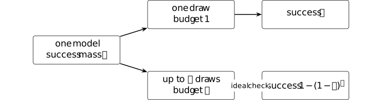
Assume independent draws and a declared perfect checker that recognizes a correct candidate when one appears. The one-draw procedure succeeds with \(J_1=p\). A procedure allowed up to \(k\) draws succeeds whenever not all draws fail: \[ J_k=1-(1-p)^k. \] Both procedures query the same conditional distribution.
Policy performance under a specified interaction and evaluation procedure is standard in [sutton2018reinforcement, Section 3.5]. The formula demonstrates procedural dependence. Independence and a perfect checker are declared toy assumptions, not properties attributed to a frontier language model.
Definition 1.1.3. Elicitation [ftip-0005]AGENTDRAFTED
Definition 1.1.3. Elicitation [ftip-0005]AGENTDRAFTED
Fix a capability claim in Convention 1.1.1, a prespecified successful behaviour event \(B\), and a tolerance \(\varepsilon >0\). Let \(p_0(B)\) be the probability of \(B\) under the declared starting procedure and \(p_1(B)\) its probability after the intervention, both measured by the same evaluator. An elicitation witness is an observed increase \[ p_1(B)>p_0(B)\quad \text {with}\quad p_0(B)\geq \varepsilon . \] It witnesses improved access to behaviour that was already observable at the declared starting budget.
The event \(B\), tolerance \(\varepsilon \), sampling procedure, and confidence rule are part of the claim. Changing any of them changes what the witness means.
Remark 1.1.4. Elicitation, starting probability, and finite evidence [ftip-0006]AGENTDRAFTED
Remark 1.1.4. Elicitation, starting probability, and finite evidence [ftip-0006]AGENTDRAFTED
Reinforcement learning can move probability toward successful traces that a base model already emits; this possibility is tested empirically in [liu2025understanding, secs. 2.3 and 3.3--3.4]. A finite experiment cannot establish that an unrestricted generative model assigns exactly zero probability to a behaviour. The positive threshold \(\varepsilon \) therefore belongs to the declared experiment rather than to an ontological claim about what the model ``contains.''
An elicitation witness depends on the sampling budget, decoding rule, and reward. Bounding the attainable increase in \(p_1(B)\) requires assumptions about the starting probability \(p_0(B)\) and the information supplied by post-training.
Definition 1.1.5. Capability acquisition [ftip-0007]AGENTDRAFTED
Definition 1.1.5. Capability acquisition [ftip-0007]AGENTDRAFTED
Fix a capability claim in Convention 1.1.1, a prespecified transfer evaluation \(E^{+}\), and thresholds \(0\leq \varepsilon _0<\varepsilon _1\leq 1\). Let \(u_0\) and \(u_1\) be the probabilities of passing \(E^{+}\) before and after the intervention, using the same evaluation protocol and budget. An acquisition witness is the pair of inequalities \[ u_0\leq \varepsilon _0 \qquad \text {and}\qquad u_1\geq \varepsilon _1. \] The transfer evaluation must not be used to select training examples, rewards, or checkpoints.
An acquisition witness is operational. It records a large, independently measured change under one declared procedure; it does not prove that the starting model assigned mathematical probability zero to every successful continuation.
Remark 1.1.6. A transfer contrast as evidence of acquisition [ftip-0008]AGENTDRAFTED
Remark 1.1.6. A transfer contrast as evidence of acquisition [ftip-0008]AGENTDRAFTED
Training success alone does not distinguish learning from memorization, selection, or evaluator exploitation. The base-versus-reinforcement-learning comparisons in [yue2025does, secs. 3--5] motivate this distinction, but their empirical criteria are not a universal definition of acquisition.
The thresholds in Definition 1.1.5 require enough evaluation samples to certify both inequalities. Whether the witness survives a distribution shift depends on the task law; evaluator leakage invalidates its interpretation as independent evidence.
1.2. Tokens, text, and probability [ftip-0009]AGENTDRAFTED
1.2. Tokens, text, and probability [ftip-0009]AGENTDRAFTED
A language model assigns probabilities to tokens rather than directly to semantic answers. We therefore fix the elementary probability notation, the text-to-token interface, and the factorization of a continuation before describing the neural computation that realizes those probabilities.
Notation 1.2.1. Finite sets, maps, distributions, random variables, and expectation [ftip-000A]AGENTDRAFTED
Notation 1.2.1. Finite sets, maps, distributions, random variables, and expectation [ftip-000A]AGENTDRAFTED
For a finite set \(X\), write \(|X|\) for its cardinality and \(X^*\) for the set of finite sequences with entries in \(X\). A map \(f:X\to Y\) sends \(x\in X\) to \(f(x)\in Y\); the inverse image of \(A\subseteq Y\) is \(f^{-1}(A)=\{x\in X:f(x)\in A\}\).
Write \[ \Delta (X)=\left \{p:X\to [0,1]:\sum _{x\in X}p(x)=1\right \} \] for the probability simplex on \(X\). If \(p\in \Delta (X)\) and \(Z:X\to \mathbb R\), then \[ \mathbb E_{x\sim p}[Z(x)]=\sum _{x\in X}p(x)Z(x). \] A random variable is a map from the sample set to its value set. Random variables \(Z\) and \(W\) are independent under \(p\) when \(p(Z=z,W=w)=p(Z=z)p(W=w)\) for every pair of values \(z,w\).
For nonfinite interaction spaces, probability laws and conditional kernels require the measurable structure described in Remark 1.2.3.
Definition 1.2.2. Finite probability law [ftip-000B]AGENTDRAFTED
Definition 1.2.2. Finite probability law [ftip-000B]AGENTDRAFTED
Using the notation of Notation 1.2.1, a finite probability law on \(X\) is an element \(p\in \Delta (X)\). For an event \(A\subseteq X\), its probability is \[ p(A)=\sum _{x\in A}p(x). \] For \(p(A)>0\), the conditional law on \(B\subseteq X\) is \(p(B\mid A)=p(A\cap B)/p(A)\).
Remark 1.2.3. Finite and measurable probability laws [ftip-000C]AGENTDRAFTED
Remark 1.2.3. Finite and measurable probability laws [ftip-000C]AGENTDRAFTED
A finite vocabulary and a bounded token sequence admit probability laws expressed as ordinary sums, with explicit normalization and conditioning. The finite-sequence interface matches [phuong2022formal, sec. 3, Sequence modelling].
States, observations, and tool outputs need not be finite. In that setting \(\Delta (X)\) is replaced by probability measures on a declared measurable space and conditional laws are probability kernels. Results on finite spaces need additional measurable-space hypotheses before they apply in this setting.
Definition 1.2.4. Finite vocabulary [phuong2022formal, sec. 3, Sequence modelling] [ftip-000D]AGENTDRAFTED
Definition 1.2.4. Finite vocabulary [phuong2022formal, sec. 3, Sequence modelling] [ftip-000D]AGENTDRAFTED
A finite vocabulary is a nonempty finite set \(\mathcal V\) of token identifiers. A token identifier is an atomic symbol for the sequence model; it need not be a word or a character.
When termination is represented in-band, choose a distinguished token \(\mathtt {eos}\in \mathcal V\). Other control tokens, if present, are named as elements of the same vocabulary rather than assumed implicitly.
Definition 1.2.5. Tokenizer and detokenizer [kudo2018sentencepiece, secs. 3.1 and 3.5] [ftip-000E]AGENTDRAFTED
Definition 1.2.5. Tokenizer and detokenizer [kudo2018sentencepiece, secs. 3.1 and 3.5] [ftip-000E]AGENTDRAFTED
Let \(\Sigma \) be a finite character or byte alphabet and let \(\mathcal V\) be the vocabulary of Definition 1.2.4. A tokenizer is a specified map \(\tau :\Sigma ^*\to \mathcal V^*\). A detokenizer is a specified map \(\delta :\mathcal V^*\to \Sigma ^*\).
A tokenizer package also fixes its text normalization rule \(N\). When the package promises normalized round trips, the relevant condition is \(\delta (\tau (s))=N(s)\) for text \(s\in \Sigma ^*\); it is not the claim that \(\tau \) and \(\delta \) are inverse bijections on all sequences. SentencePiece keeps the segmentation model and detokenization convention together, which is why both maps belong to the model interface.
Byte-pair encoding gives another construction of \(\tau \). Learned merge operations turn an initial symbol sequence into subword units; see [sennrich2016neural, §3.2]. The learned merges and base alphabet are therefore part of the tokenizer specification.
Example 1.2.6. A tokenizer round trip and normalization failure [ftip-000F]AGENTDRAFTED
Example 1.2.6. A tokenizer round trip and normalization failure [ftip-000F]AGENTDRAFTED
A four-stage toy tokenizer separates token-level round-trip stability from recovery of the original string.

Here underscores display spaces. Declare \(N(A\_\_B)=a\_b\), \(T(a\_b)=(a,b)\), and \(D(a,b)=a\_b\). For \(s=A\_\_B\), \[ D(T(N(s)))=a\_b\neq s, \qquad T(N(D(T(N(s)))))=(a,b). \] The token sequence is stable after normalization although the original case and repeated space are not recovered.
The source-grounded tokenizer interface is Definition 1.2.5. The displayed normalization rule belongs only to this finite construction; no such lossy transformation is attributed to SentencePiece.
Convention 1.2.7. Token sequences, prefixes, positions, and end-of-sequence [ftip-000G]AGENTDRAFTED
Convention 1.2.7. Token sequences, prefixes, positions, and end-of-sequence [ftip-000G]AGENTDRAFTED
Let \(\mathcal V\) be the vocabulary of Definition 1.2.4. A token sequence of length \(n\geq 0\) is written \(x_{1:n}=(x_1,\ldots ,x_n)\in \mathcal V^n\); positions are one-based. Its length is \(|x_{1:n}|=n\), its prefix before position \(t\) is \(x_{<t}=x_{1:t-1}\), and \(x_{<1}\) is the empty sequence. Juxtaposition \(xy\) denotes concatenation.
If \(\mathtt {eos}\) is distinguished, a completed generated continuation \(y_{1:m}\) ends with \(y_m=\mathtt {eos}\) and contains no earlier \(\mathtt {eos}\). A fixed length limit can also stop generation; the stopping mechanism must state which convention it uses.
Definition 1.2.8. Conditional next-token law [phuong2022formal, sec. 3, Sequence modelling] [ftip-000H]AGENTDRAFTED
Definition 1.2.8. Conditional next-token law [phuong2022formal, sec. 3, Sequence modelling] [ftip-000H]AGENTDRAFTED
Let \(\Theta \) be a parameter set. With the probability notation of Notation 1.2.1 and the sequence convention of Convention 1.2.7, a conditional next-token law is a family of maps \[ \pi _\theta :\mathcal V^*\longrightarrow \Delta (\mathcal V), \qquad \theta \in \Theta . \] For a prefix \(x_{<t}\) and token \(a\in \mathcal V\), the number \(\pi _\theta (a\mid x_{<t})\) is the probability assigned to choosing \(a\) at position \(t\).
This is the observable probabilistic interface. It does not yet specify the neural computation that produces the distribution.
Definition 1.2.9. Autoregressive continuation law [phuong2022formal, sec. 3, Sequence modelling] [ftip-000I]AGENTDRAFTED
Definition 1.2.9. Autoregressive continuation law [phuong2022formal, sec. 3, Sequence modelling] [ftip-000I]AGENTDRAFTED
Fix the next-token law of Definition 1.2.8, a prompt \(x\in \mathcal V^*\), and a continuation \(y_{1:m}\in \mathcal V^m\). Its autoregressive continuation probability is \[ P_\theta (y_{1:m}\mid x) =\prod _{t=1}^{m} \pi _\theta \left (y_t\mid x y_{<t}\right ). \] Each factor conditions only on the prompt and earlier continuation tokens.
If generation stops on \(\mathtt {eos}\), the law of a completed continuation is restricted to the sequences specified in Convention 1.2.7. If generation instead stops at a length limit, the terminal event and its probability must be recorded separately.
Example 1.2.10. A three-symbol autoregressive continuation [ftip-000J]AGENTDRAFTED
Example 1.2.10. A three-symbol autoregressive continuation [ftip-000J]AGENTDRAFTED
Along one branch of a three-symbol prefix tree, conditional token laws determine both continuation probability and negative log-likelihood.

Let the vocabulary be \(\{a,b,\mathtt {EOS}\}\) and let \(p_i\) be the displayed conditional probability at step \(i\). The continuation \((b,a,\mathtt {EOS})\) has \[ \Pr (b,a,\mathtt {EOS}\mid a) =p_1p_2p_3, \qquad -\log \Pr =-\sum _{i=1}^{3}\log p_i. \]
The multiplication follows the causal product in [phuong2022formal, Section 3]. Its scope is one fixed finite continuation, leaving both the decoding algorithm and the law over all variable-length outputs unspecified.
1.3. Pretraining [ftip-0014]AGENTDRAFTED
1.3. Pretraining [ftip-0014]AGENTDRAFTED
Pretraining fits the parameters of a language model to a large corpus by predicting tokens from preceding tokens. This description leaves the data law, window sampler, loss mask, population objective, finite-sample objective, and update rule unspecified. Each receives a separate definition below.
Notation 1.3.1. Pretraining data, masks, parameters, and updates [ftip-0015]AGENTDRAFTED
Notation 1.3.1. Pretraining data, masks, parameters, and updates [ftip-0015]AGENTDRAFTED
Let \(\mathcal D_{\rm doc}\) be a measurable document space and \(\mathcal S\) a finite set of data sources. Source \(s\in \mathcal S\) has a document law \(Q_s\) on \(\mathcal D_{\rm doc}\), and mixture weights \(\alpha \in \Delta (\mathcal S)\) use the simplex notation of Notation 1.2.1. Let \(T\) be the context length. A token window is \(x_{1:T}\in \mathcal V^T\); a prediction mask is \(m_{1:T}\in \{0,1\}^T\), where \(m_t=1\) means that the token at position \(t\) contributes to the loss.
Let \(\Theta \) be the parameter set used by the next-token law in Definition 1.2.8. The model parameters at optimizer update \(k\in \{0,1,\ldots ,K\}\) are \(\theta _k\in \Theta \); \(\theta _0\) is the initialization and \(\theta _K\) the stopped parameter value. A minibatch at update \(k\) is \(\mathcal B_k\). Random document draws, window offsets, masks, batch order, and optimizer noise are part of the training run even when the notation suppresses them.
Definition 1.3.2. Pretraining source mixture [ftip-0016]AGENTDRAFTED
Definition 1.3.2. Pretraining source mixture [ftip-0016]AGENTDRAFTED
Using Notation 1.3.1, a pretraining source mixture is the pair \(((Q_s)_{s\in \mathcal S},\alpha )\). It induces the document law \[ Q_{\alpha }(A)=\sum _{s\in \mathcal S}\alpha _s Q_s(A) \] for every document event \(A\): first sample a source \(s\) with probability \(\alpha _s\), then sample a document from \(Q_s\).
The mixture weights specify sampling frequency. They need not equal the fraction of bytes stored in each source. Resampling, epoch boundaries, or temperature-based weights must therefore be recorded as part of \(\alpha \) or its schedule.
Definition 1.3.3. Document filter [ftip-0070]AGENTDRAFTED
Definition 1.3.3. Document filter [ftip-0070]AGENTDRAFTED
Let \(\dagger \) denote rejection. A document filter is a declared map \[ F:\mathcal D_{\rm doc}\longrightarrow \mathcal D_{\rm doc}\cup \{\dagger \}. \] It may retain a document, return a transformed document, or reject it. The lift \(F_{\#}\) applies \(F\) to a finite corpus and removes every \(\dagger \).
A filter specification includes the features it reads, thresholds, transformation rules, and implementation revision. An acceptance rate alone does not determine the retained document law.
Definition 1.3.4. Deduplication operator [ftip-0071]AGENTDRAFTED
Definition 1.3.4. Deduplication operator [ftip-0071]AGENTDRAFTED
Let \(\mathcal M_{\rm doc}\) be the set of finite multisets of documents. A deduplication operator is a map \[ D:\mathcal M_{\rm doc}\longrightarrow \mathcal M_{\rm doc} \] that selects retained representatives according to a declared duplicate relation. The relation may compare complete documents or spans.
The declaration includes normalization, similarity threshold, cluster construction, and representative tie-breaking. Different choices can remove different training events even when they report the same duplicate rate.
Definition 1.3.5. Evaluation decontamination operator [ftip-0072]AGENTDRAFTED
Definition 1.3.5. Evaluation decontamination operator [ftip-0072]AGENTDRAFTED
For a protected evaluation collection \(\mathcal E\), an evaluation decontamination operator is a map \[ C_{\mathcal E}:\mathcal M_{\rm doc}\longrightarrow \mathcal M_{\rm doc} \] that removes documents or spans matching \(\mathcal E\) under a declared matching rule.
The protected collection, normalization, match granularity, threshold, and removal policy are part of the operator. Decontamination against one released benchmark does not establish independence from every related task.
Definition 1.3.6. Ordered pretraining data pipeline [ftip-0017]AGENTDRAFTED
Definition 1.3.6. Ordered pretraining data pipeline [ftip-0017]AGENTDRAFTED
Let \(\mathcal C_{\mathrm {raw}}\in \mathcal M_{\rm doc}\) be a finite corpus drawn from the source mixture in Definition 1.3.2. Using the declared document filter, deduplication operator, and evaluation decontamination operator, an ordered pretraining data pipeline returns \[ \mathcal C_{\mathrm {clean}} =C_{\mathcal E}\left (D\left (F_{\#}(\mathcal C_{\mathrm {raw}})\right )\right ). \] Changing the order can change the retained corpus. The pipeline therefore records the order and exact revisions in addition to the three operators.
Remark 1.3.7. From a data pipeline to a corpus law [ftip-0018]AGENTDRAFTED
Remark 1.3.7. From a data pipeline to a corpus law [ftip-0018]AGENTDRAFTED
The source mixture and cleaning pipeline determine different parts of the data law. The mixture in Definition 1.3.2 describes how raw documents are proposed. The construction in Definition 1.3.6 determines which proposals survive and how they are transformed. Together with all random seeds and thresholds, they induce a cleaned document law \(Q_{\mathrm {clean}}\).
Kaplan et al. describe the concrete WebText2 dataset in [kaplan2020scaling, sec. 2.3]. Hoffmann et al. report the MassiveText sources and mixture in [hoffmann2022training, Appendix A, Table A1]. A finite released corpus is one realization of such choices, and an undocumented change in them is not identified by a loss--compute curve.
Definition 1.3.8. Context-window sampler [ftip-0019]AGENTDRAFTED
Definition 1.3.8. Context-window sampler [ftip-0019]AGENTDRAFTED
Fix the context length \(T\) from Notation 1.3.1. A context-window sampler draws cleaned text from the law described in Remark 1.3.7 and tokenizes it with Definition 1.2.5. It then chooses a declared offset and returns a length-\(T\) token sequence \(x_{1:T}\) together with metadata that identifies document boundaries.
If fewer than \(T\) tokens remain, the sampler must specify whether it pads, drops the suffix, or joins another document. These choices change both the distribution of contexts and the prediction mask.
Definition 1.3.9. Sequence packing and document mask [ftip-001A]AGENTDRAFTED
Definition 1.3.9. Sequence packing and document mask [ftip-001A]AGENTDRAFTED
A packed training record is a tuple \(\zeta =(x,m,c,M^{\mathrm {doc}})\). It places tokenized segments \(x^{(1)},\ldots ,x^{(r)}\) into the length-\(T\) token array \(x\), records a prediction mask \(m\), and records a segment identifier \(c_t\in \{0,1,\ldots ,r\}\) at each position. The value \(c_t=0\) denotes padding. Its document mask is \[ M^{\mathrm {doc}}_{ts}= \begin {cases} 0,&c_t=c_s\ne 0\text { and }s\leq t,\\ -\infty ,&\text {otherwise}. \end {cases} \] Replacing the causal mask in Definition 5.1.8 by this mask prevents one packed document from attending to another. We write \(x_t(\zeta )\), \(m_t(\zeta )\), and \(M^{\mathrm {doc}}(\zeta )\) for the corresponding fields.
The prediction mask \(m_t(\zeta )\) from Notation 1.3.1 is one only at positions whose target token is retained for training. Padding, a segment's first token when no predecessor is present, and any deliberately excluded control token receive mask value zero.
Remark 1.3.10. Window sampling, document masks, and packing [ftip-006K]AGENTDRAFTED
Remark 1.3.10. Window sampling, document masks, and packing [ftip-006K]AGENTDRAFTED
[kaplan2020scaling], Section 2.2, uses fixed-length sequence batches.
[phuong2022formal], Section 7, gives the causal language-model objective.
The proposed data interface additionally specifies the sampler, segment identifiers, document mask, and prediction mask. Those boundary choices are not determined by the high-level training accounts.
These objects describe one admissible data interface. A concrete training run must replace them with its offset, padding, joining, masking, and packing rules.
Definition 1.3.11. Token negative log-likelihood [ftip-001B]AGENTDRAFTED
Definition 1.3.11. Token negative log-likelihood [ftip-001B]AGENTDRAFTED
Let \(\zeta =(x,m,c,M^{\mathrm {doc}})\) be a packed training record from Definition 1.3.9. Write \(\pi _{\theta ,M^{\mathrm {doc}}(\zeta )}(\,\cdot \mid x_{<t}(\zeta ))\) for the next-token law of Definition 1.2.8 when every decoder attention layer uses the declared document mask. For a predicted position \(t\geq 2\), its masked token negative log-likelihood is \[ \ell _t(\theta ;\zeta ) =-m_t(\zeta )\log \pi _{\theta ,M^{\mathrm {doc}}(\zeta )} \left (x_t(\zeta )\mid x_{<t}(\zeta )\right ), \] A masked position has zero contribution; an unmasked position penalizes the log probability computed under the same segment boundaries that defined the packed example.
Definition 1.3.12. Population pretraining objective [ftip-001C]AGENTDRAFTED
Definition 1.3.12. Population pretraining objective [ftip-001C]AGENTDRAFTED
Let \(Q_T\) be the law of packed examples induced by Remark 1.3.7--Definition 1.3.9, and assume that its expected number of predicted positions is positive. The population pretraining objective is the expected total token loss divided by the expected number of predicted tokens: \[ L_{\mathrm {pop}}(\theta ) =\frac { \mathbb E_{\zeta \sim Q_T} \left [\sum _{t=2}^{T}\ell _t(\theta ;\zeta )\right ] }{ \mathbb E_{\zeta \sim Q_T} \left [\sum _{t=2}^{T}m_t(\zeta )\right ] }, \] using expectation as fixed in Notation 1.2.1.
Example 1.3.13. Packing two documents without cross-document attention [ftip-001D]AGENTDRAFTED
Example 1.3.13. Packing two documents without cross-document attention [ftip-001D]AGENTDRAFTED
Packing documents into one row requires a block-causal mask so that each token attends only within its own document and to earlier positions there.

For a packed row, set \(M_{ij}=0\) only when tokens \(i,j\) belong to the same document and \(j\leq i\); otherwise set \(M_{ij}=-\infty \). Thus a token in document \(B\) cannot inspect any token in document \(A\), even when \(A\) precedes \(B\) in storage.
The within-document triangle instantiates the causal mask in Definition 5.1.8. The block boundary instantiates the packing convention in Definition 1.3.9. Document-isolated attention is the declared convention in this packed row, not a universal description of pretraining systems.
Definition 1.3.14. Empirical pretraining objective [ftip-001E]AGENTDRAFTED
Definition 1.3.14. Empirical pretraining objective [ftip-001E]AGENTDRAFTED
For a finite training sample of packed records \(\mathcal D_N=(\zeta ^{(i)})_{i=1}^{N}\) with at least one unmasked target token, the empirical pretraining objective is \[ L_N(\theta ) =\frac { \sum _{i=1}^{N}\sum _{t=2}^{T} \ell _t(\theta ;\zeta ^{(i)}) }{ \sum _{i=1}^{N}\sum _{t=2}^{T}m_t(\zeta ^{(i)}) }. \] This is a per-predicted-token average. Reusing or resampling examples changes the stochastic optimization path even when the displayed finite-sample function is unchanged.
Remark 1.3.15. Normalization of masked pretraining loss [ftip-006L]AGENTDRAFTED
Remark 1.3.15. Normalization of masked pretraining loss [ftip-006L]AGENTDRAFTED
The autoregressive token loss follows [phuong2022formal, Section 7]. Kaplan et al. report language-model loss with parameter and compute variables in [kaplan2020scaling, sec. 2.1]. The population ratio-of-expectations in Definition 1.3.12 and finite per-token ratio in Definition 1.3.14 are proposed normalization conventions with explicit prediction masks. Neither cited source defines those exact ratios.
A theorem or experiment using another record weighting, length weighting, or expectation order must state that change rather than reuse these symbols.
Definition 1.3.16. Minibatch gradient estimator [ftip-001G]AGENTDRAFTED
Definition 1.3.16. Minibatch gradient estimator [ftip-001G]AGENTDRAFTED
At update \(k\), let \(\mathcal B_k\) be the minibatch named in Notation 1.3.1, and let \(N_k=\sum _{\zeta \in \mathcal B_k}\sum _{t=2}^{T}m_t(\zeta )\) be its number of predicted tokens. For \(N_k>0\), the minibatch gradient estimator is \[ g_k=\frac 1{N_k} \sum _{\zeta \in \mathcal B_k}\sum _{t=2}^{T} \nabla _\theta \ell _t(\theta _k;\zeta ), \] where \(\ell _t\) is defined in Definition 1.3.11. Whether \(g_k\) is unbiased for the gradient of Definition 1.3.12 depends on the window sampler and minibatch weighting. Other sampling schemes require their own bias statement.
Example 1.3.17. A two-record pretraining loss and minibatch estimate [ftip-001F]AGENTDRAFTED
Example 1.3.17. A two-record pretraining loss and minibatch estimate [ftip-001F]AGENTDRAFTED
Two equal-length records make a full empirical loss directly comparable with a minibatch estimate, while exposing the assumptions behind unbiasedness.
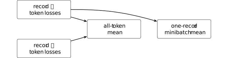
Let \(\ell _{ij}\) denote the token loss at position \(j\) of record \(i\). The full token-average loss is the mean of all \(\ell _{ij}\), while a one-record minibatch averages only the losses from its sampled record. Uniform sampling of equal-length records makes the latter unbiased for the former.
The preceding loss and estimator definitions apply to this equal-length record setup. Equal record lengths make the estimator unbiased here; unequal lengths, padding, dependence, and optimizer noise remain outside its scope.
Definition 1.3.18. Optimizer state [kingma2015adam, Algorithm 1] [ftip-001H]AGENTDRAFTED
Definition 1.3.18. Optimizer state [kingma2015adam, Algorithm 1] [ftip-001H]AGENTDRAFTED
An optimizer state \(s_k\) is the collection of persistent variables, other than the model parameters \(\theta _k\), that an update rule uses after step \(k\). For Adam, \(s_k\) contains the step index and exponential moving averages of the gradient and squared gradient.
The state is initialized by a declared value \(s_0\). Two runs with the same checkpoint \(\theta _k\) but different optimizer states need not have the same next update.
Definition 1.3.19. Parameter update [kingma2015adam, Algorithm 1] [ftip-001I]AGENTDRAFTED
Definition 1.3.19. Parameter update [kingma2015adam, Algorithm 1] [ftip-001I]AGENTDRAFTED
A parameter update rule is a specified map \(U_k\) that takes the current parameters \(\theta _k\), optimizer state \(s_k\), gradient estimate \(g_k\), and scheduled hyperparameters \(\eta _k\), and returns \[ (\theta _{k+1},s_{k+1}) =U_k(\theta _k,s_k,g_k,\eta _k). \] The learning rate, momentum coefficients, numerical stabilizers, clipping, and weight decay belong to \(\eta _k\) or to the declared form of \(U_k\); they are not determined by the loss alone.
Remark 1.3.20. Randomness, schedules, and stopping [ftip-001J]AGENTDRAFTED
Remark 1.3.20. Randomness, schedules, and stopping [ftip-001J]AGENTDRAFTED
A pretraining run is not determined by minimization of the empirical objective \(L_N\) in Definition 1.3.14. It includes the initialization, data order, window offsets, dropout and other model randomness, numerical precision, distributed reduction order, optimizer state, every hyperparameter schedule, and a stopping rule. These objects determine a distribution over final parameters even when the source mixture and nominal objective agree.
The training configuration of [vaswani2017attention, sec. 5.3] and the scaling experiments of [kaplan2020scaling, sec. 2.2] report concrete instances of these choices. An optimization result depends on which randomness it averages over and whether the stopping time is fixed or data-dependent.
Definition 1.3.21. Base-model artifact [ftip-001K]AGENTDRAFTED
Definition 1.3.21. Base-model artifact [ftip-001K]AGENTDRAFTED
A base-model artifact is an executable tuple \[ M_0=(\tau ,\delta ,\mathsf {cfg},\theta _K,\mathsf {num}), \] where \(\tau ,\delta \) are the tokenizer and detokenizer of Definition 1.2.5; \(\mathsf {cfg}\) fixes the architecture of Definition 5.1.21; \(\theta _K\) is the stopped pretraining checkpoint; and \(\mathsf {num}\) fixes the numerical and inference conventions required to evaluate its next-token law.
The tokenizer model is part of the executable system by Definition 1.2.5. A weight file without its vocabulary, architecture configuration, or output convention does not determine the law \(\pi _{\theta _K}\) in Definition 1.2.8. Training-data and optimizer provenance may accompany the artifact, but they are not runtime inputs.
Remark 1.3.22. The runtime ingredients of a model artifact [ftip-006M]AGENTDRAFTED
Remark 1.3.22. The runtime ingredients of a model artifact [ftip-006M]AGENTDRAFTED
Section 6 of [phuong2022formal] describes decoder architecture. Sections 3.1 and 3.5 of [kudo2018sentencepiece] treat the tokenizer as a separate model. Public model releases additionally distribute weights, configuration, and numerical conventions. The proposed artifact model in Definition 1.3.21 includes these runtime ingredients because none alone determines an executable next-token law.
Training provenance accompanies the artifact but is not itself a runtime argument. Later causal claims must distinguish the executable endpoint from the process that produced it.
Example 1.3.23. Anatomy of a base-model artifact and V4 optimizer/data provenance [ftip-001L]AGENTDRAFTED
Example 1.3.23. Anatomy of a base-model artifact and V4 optimizer/data provenance [ftip-001L]AGENTDRAFTED
An executable-artifact manifest separates runtime components from evidence about how the corresponding weights were trained.
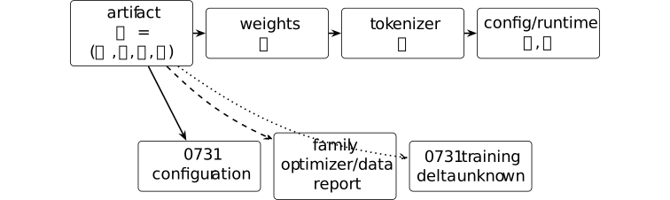
The pinned DeepSeek-V4-Flash-0731 configuration [⧉] declares architecture and numeric-format fields. Sections 2.4 and 4 of the V4 family report [⧉] describe a mixed Muon/AdamW optimizer allocation and pretraining data construction. The exact 0731 data mixture, optimizer schedule, and post-preview training delta remain undisclosed by those sources.
1.4. Tasks and evaluation interfaces [ftip-001M]AGENTDRAFTED
1.4. Tasks and evaluation interfaces [ftip-001M]AGENTDRAFTED
A model does not have a benchmark score without a task distribution, an inference procedure, and an evaluator. Keeping these objects separate is essential for post-training: a training change and an evaluation-time search change can raise the same reported score while answering different research questions.
Notation 1.4.1. Tasks, task laws, inference protocols, and utility [ftip-001N]AGENTDRAFTED
Notation 1.4.1. Tasks, task laws, inference protocols, and utility [ftip-001N]AGENTDRAFTED
Write \(\mathsf T\) for a task interface, \(\mathcal X_{\mathsf T}\) for its instance set, and \(\mathcal O_{\mathsf T}\) for its candidate-outcome set. A task instance is \(x\in \mathcal X_{\mathsf T}\) and a candidate outcome is \(o\in \mathcal O_{\mathsf T}\). The symbol \(\mu _{\mathsf T}\) denotes a probability law on instances. Equip the instance and outcome sets with declared sigma-algebras; \(\mu _{\mathsf T}\) is a probability measure on the instance sigma-algebra.
Fix an evaluation-resource dimension \(m_{\mathrm {eval}}\geq 1\) and write \(\mathcal B_{\mathrm {eval}}=\mathbb R_+^{m_{\mathrm {eval}}}\) with its coordinatewise order. An evaluation inference protocol is written \(\mathsf I\); its declared evaluation budget is \(b_{\mathrm {eval}}\in \mathcal B_{\mathrm {eval}}\). Its inference-seed set is \(\Omega _I\), with realized seed \(\xi \in \Omega _I\). An evaluator's random-seed set is \(\Omega _E\); its realized seed is \(\omega \in \Omega _E\). It returns utility \(u_{\mathsf T}(x,o;\omega )\in \mathbb R^d\). The dimension \(d\geq 1\) is declared by the evaluation: \(d=1\) gives scalar utility, while \(d>1\) retains several outcomes or costs without an implicit weighting. Equip both seed sets with declared sigma-algebras and \(\mathbb R^d\) with its Borel sigma-algebra. Products below carry the product sigma-algebra; finite or countable discrete spaces may use all subsets. A seed space alone does not specify its sampling law.
Definition 1.4.2. Task [ftip-001O]AGENTDRAFTED
Definition 1.4.2. Task [ftip-001O]AGENTDRAFTED
A task is a triple \[ \mathsf T=(\mathcal X_{\mathsf T},\mathcal O_{\mathsf T}, \operatorname {Adm}_{\mathsf T}), \] where \(\mathcal X_{\mathsf T}\) is an instance set, \(\mathcal O_{\mathsf T}\) is a candidate-outcome set, and \(\operatorname {Adm}_{\mathsf T}(x,o)\) is a declared well-formedness predicate for an instance-outcome pair.
Admissibility says that an outcome can be interpreted for the instance; it does not say that the outcome is correct, useful, or safe. Those judgments belong to the evaluation utility introduced later.
Definition 1.4.3. Task law [ftip-001Q]AGENTDRAFTED
Definition 1.4.3. Task law [ftip-001Q]AGENTDRAFTED
For the instance set in Definition 1.4.2, a task law is a probability law \(\mu _{\mathsf T}\) on \(\mathcal X_{\mathsf T}\). An evaluation sample of size \(N\) is a declared joint law of instances \((X_1,\ldots ,X_N)\) whose marginals are \(\mu _{\mathsf T}\); independent sampling is a further assumption, not part of the term ``task law.''
In an episodic control problem this law includes the distribution of starting situations. In a fixed benchmark it may instead be the uniform law on a held-out finite set. Reweighting instances changes the task law even when the instance files are unchanged.
Remark 1.4.4. Response tasks and interactive tasks [ftip-001P]AGENTDRAFTED
Remark 1.4.4. Response tasks and interactive tasks [ftip-001P]AGENTDRAFTED
A task and a task law specify admissible instance--outcome pairs and how instances are sampled. Benchmark datasets usually present an input and expect an answer in a parseable format. Reinforcement-learning formulations instead name states, actions, and reward; see [sutton2018reinforcement, Chapter 3]. The admissibility predicate captures parseability, while the law records how instances are sampled. Neither choice already identifies parsing with success.
One-shot inference and an interactive environment can share the same task interface. Claims about an interaction's temporal structure additionally depend on the environment and the observations available at each decision.
Definition 1.4.5. Evaluation inference protocol [ftip-001R]AGENTDRAFTED
Definition 1.4.5. Evaluation inference protocol [ftip-001R]AGENTDRAFTED
Let \(M\) be an executable model artifact of the form in Definition 1.3.21. An evaluation inference protocol is a specified procedure \[ \mathsf I(M,x,b_{\mathrm {eval}};\xi )=(o,c) \in \mathcal O_{\mathsf T}\times \mathcal B_{\mathrm {eval}}, \] where \(x\in \mathcal X_{\mathsf T}\), \(b_{\mathrm {eval}}\in \mathcal B_{\mathrm {eval}}\), and \(\xi \in \Omega _I\) use the notation of Notation 1.4.1; \(o\) is a candidate outcome and \(c\in \mathcal B_{\mathrm {eval}}\) is the realized resource-use vector. A valid execution satisfies \(c\preceq b_{\mathrm {eval}}\) coordinatewise.
The protocol fixes prompt construction, decoding, sampling temperature, number of candidates, candidate selection, allowed tools, stopping, and any test-time search. None of these choices is determined by the checkpoint alone.
Remark 1.4.6. Decoding and test-time compute belong to evaluation [ftip-001S]AGENTDRAFTED
Remark 1.4.6. Decoding and test-time compute belong to evaluation [ftip-001S]AGENTDRAFTED
One next-token law supports many evaluation procedures. Greedy decoding, temperature sampling, majority voting, verifier-guided selection, and multi-round tool use can produce different outcome laws from the same checkpoint. The sampling and selection procedures in [shao2024deepseekmath, secs. 3--4] are concrete examples.
Accordingly, a comparison that changes \(b_{\mathrm {eval}}\) or \(\mathsf I\) does not estimate a training-only effect. A potential frontier therefore depends on evaluation-time compute as well as the trained model.
Definition 1.4.7. Evaluation utility [ftip-001T]AGENTDRAFTED
Definition 1.4.7. Evaluation utility [ftip-001T]AGENTDRAFTED
With the notation of Notation 1.4.1, an evaluation utility is a declared measurable function \[ u_{\mathsf T}:\mathcal X_{\mathsf T}\times \mathcal O_{\mathsf T}\times \Omega _E\longrightarrow \mathbb R^d, \] where \(\Omega _E\) is the evaluator's measurable seed space. The evaluator applies it only to admissible pairs from Definition 1.4.2. A deterministic evaluator is the special case in which the value does not depend on \(\omega \in \Omega _E\).
Binary pass-fail evaluation takes \(d=1\) and values in \(\{0,1\}\). A cumulative return is another scalar case. Vector utility keeps qualities such as correctness, safety, latency, and tool cost distinct until a later rule declares how to compare them.
Whenever an expected utility vector is used, its composite evaluation random variable must be measurable and absolutely integrable in every coordinate under the declared joint law. Thus its expectation lies in \(\mathbb R^d\). Bounded measurable utility is a sufficient specialization; so is finite support for the complete evaluation random variable with finite values on that support. Merely taking a finite real value at each seed is insufficient for an unbounded evaluator. The scalar protocol comparison in Convention 4.1.1 states its joint law explicitly.
Remark 1.4.8. Scalar returns and multiple evaluation quantities [ftip-006N]AGENTDRAFTED
Remark 1.4.8. Scalar returns and multiple evaluation quantities [ftip-006N]AGENTDRAFTED
Sutton and Barto define scalar episodic return in [sutton2018reinforcement, Section 3.3]. Benchmarks also use exact-match, test, latency, safety, and cost measurements. A proposed seeded vector utility keeps those coordinates separate, with evaluator randomness included in the declared law.
The vector is not a claim that its coordinates share a natural scale. Scalarization, Pareto order, and worst-group summaries are introduced only after the attainable evaluation set is defined.
Example 1.4.9. One policy under two evaluation inference budgets [ftip-001U]AGENTDRAFTED
Example 1.4.9. One policy under two evaluation inference budgets [ftip-001U]AGENTDRAFTED
One fixed policy can receive different measured success rates when the evaluation horizon changes.
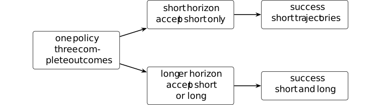
Partition complete trajectories into those that finish within the short horizon, those requiring additional tokens, and failures. The short protocol counts only the first class; the longer protocol may count the first two. Thus the measured score depends on the declared horizon even though the policy is unchanged.
Making an evaluation horizon explicit follows finite-horizon policy evaluation in [sutton2018reinforcement, Chapter 3]. Only truncation is varied here. Larger budgets need not help once decoding rules, tool costs, or selection errors are allowed to change with the budget.
Remark 1.4.10. Public task data and evaluator-only information [ftip-001V]AGENTDRAFTED
Remark 1.4.10. Public task data and evaluator-only information [ftip-001V]AGENTDRAFTED
The inference protocol receives only the information designated as public. The public instance \(x\) may include a prompt, tools, and a response schema. Evaluator-only information may include a reference answer, hidden tests, a simulator state, or the evaluator seed \(\omega \). The protocol in Definition 1.4.5 receives the former and not the latter.
If evaluator-only information influences training, decoding, or candidate selection, the experiment no longer measures performance under the declared information interface. A theorem that assumes an independent evaluator must name the sigma-field or finite data record from which the protocol is excluded.
1.5. Interactive environments and policies [ftip-001W]AGENTDRAFTED
1.5. Interactive environments and policies [ftip-001W]AGENTDRAFTED
Some tasks end with one generated response. Agentic tasks instead alternate between an acting system and an environment: the system calls a tool, receives an observation, and chooses what to do next. The following objects make that temporal and informational structure explicit before any reinforcement-learning objective is introduced.
Notation 1.5.1. State, observation, action, time, history, and stopping [ftip-001X]AGENTDRAFTED
Notation 1.5.1. State, observation, action, time, history, and stopping [ftip-001X]AGENTDRAFTED
Let \(\mathcal S,\mathcal O,\mathcal A\) be declared measurable spaces of environment states, public observations, and agent actions. Time is discrete, \(t\in \{0,1,\ldots ,T_{\max }\}\), where \(T_{\max }<\infty \) is a hard horizon. Random states, observations, and actions are \(S_t,O_t,A_t\); lowercase \(s_t,o_t,a_t\) denote realized values. The same convention makes \(h_t\) a realization of \(H_t\) and \(z\) a realization of \(Z\).
The public history available before action \(A_t\) is \(H_t\); the full environment trajectory is \(Z\); and the stopping time is \(\tau _{\mathrm {stop}}\in \{0,1,\ldots ,T_{\max }\}\). Probability kernels are written \(K(dy\mid x)\); on finite spaces this means the probability law \(K(y\mid x)\) and reduces to the notation of Notation 1.2.1.
Definition 1.5.2. Initial-state law [ftip-001Y]AGENTDRAFTED
Definition 1.5.2. Initial-state law [ftip-001Y]AGENTDRAFTED
With the spaces in Notation 1.5.1, an initial-state law \(\rho _0(ds_0,do_0)\) is a probability law on \(\mathcal S\times \mathcal O\). It jointly samples the hidden initial state \(S_0\) and the first public observation \(O_0\).
Allowing a joint law covers both a deterministic rendering \(O_0=\operatorname {obs}(S_0)\) and a noisy initial observation. A fixed task instance can be included as a coordinate of \(O_0\); its sampling law is then the task law of Definition 1.4.3.
Definition 1.5.3. Transition-observation kernel [ftip-001Z]AGENTDRAFTED
Definition 1.5.3. Transition-observation kernel [ftip-001Z]AGENTDRAFTED
A transition-observation kernel at time \(t\) is a probability kernel \[ K_t(ds_{t+1},do_{t+1}\mid s_t,a_t) \] from the current hidden state and action to the next hidden state and public observation. After \(A_t=a_t\), the environment draws \((S_{t+1},O_{t+1})\) from this kernel.
The factorization \(K_t(ds',do'\mid s,a)=P_t(ds'\mid s,a)\,Q_t(do'\mid s',a)\) for declared kernels \(P_t\) and \(Q_t\) recovers the usual separate state-transition and observation kernels when such a factorization is declared. The joint-kernel form does not assume it.
Remark 1.5.4. Deterministic tools and stochastic environments [ftip-0020]AGENTDRAFTED
Remark 1.5.4. Deterministic tools and stochastic environments [ftip-0020]AGENTDRAFTED
The kernel in Definition 1.5.3 describes both tools and broader environments. A deterministic tool has a measurable update map \(F_t(s,a)=(s',o')\) and the point-mass kernel concentrated at \(F_t(s,a)\). A stochastic environment permits several next state-observation pairs for the same input.
This distinction matters for replay. Re-executing a deterministic tool call under an unchanged state reproduces its observation, whereas a stored rollout from a stochastic environment is one sample from a conditional law. Any analysis that replaces one with the other needs a coupling or concentration assumption.
Definition 1.5.5. Public history [ftip-0021]AGENTDRAFTED
Definition 1.5.5. Public history [ftip-0021]AGENTDRAFTED
At time \(t\), the public history is the alternating sequence \[ H_t=(O_0,A_0,O_1,A_1,\ldots ,A_{t-1},O_t). \] Thus \(H_0=(O_0)\). It contains exactly the observations received and actions taken before the next action \(A_t\); it does not contain the hidden state \(S_t\) unless that state was itself revealed as an observation.
Remark 1.5.6. The information boundary of a history [ftip-0022]AGENTDRAFTED
Remark 1.5.6. The information boundary of a history [ftip-0022]AGENTDRAFTED
The history in Definition 1.5.5 contains the agent's available information. The hidden state sequence \((S_0,\ldots ,S_t)\), future observations, evaluator-only tests from Remark 1.4.10, and future random seeds are absent unless the environment has already exposed them through \(O_0,\ldots ,O_t\).
This boundary determines which policies are implementable. It also separates legitimate memory from leakage: a summary of earlier public observations may be stored in the history, while a hidden reference answer may not be supplied under the same declaration.
Definition 1.5.7. Non-anticipating policy [ftip-0023]AGENTDRAFTED
Definition 1.5.7. Non-anticipating policy [ftip-0023]AGENTDRAFTED
A non-anticipating policy is a family of probability kernels \[ \pi _t(da\mid H_t), \qquad t=0,1,\ldots ,T_{\max }-1, \] from public histories in Definition 1.5.5 to the action space \(\mathcal A\). At time \(t\), the action may depend on \(H_t\) and fresh policy randomness, but not on a later observation or an unobserved state.
A decoder-only language model becomes such a policy only after an inference protocol serializes \(H_t\) into tokens, decodes tokens, and parses them as an action. The next-token law in Definition 1.2.8 alone does not specify those maps.
Definition 1.5.8. Stopping rule [ftip-0024]AGENTDRAFTED
Definition 1.5.8. Stopping rule [ftip-0024]AGENTDRAFTED
A stopping rule is a random time \(\tau _{\mathrm {stop}}\in \{0,1,\ldots ,T_{\max }\}\) such that, for each \(t\), the decision whether \(\tau _{\mathrm {stop}}=t\) is determined by the public history \(H_t\) and any declared stopping randomness available by time \(t\). It cannot inspect future observations.
Stopping can be triggered by a terminal environment observation, an agent action, a resource limit, or the hard horizon. The trigger and the owner of the decision are part of the rule.
Definition 1.5.9. Stopped trajectory [ftip-0025]AGENTDRAFTED
Definition 1.5.9. Stopped trajectory [ftip-0025]AGENTDRAFTED
If \(\tau _{\mathrm {stop}}=n\), the stopped trajectory is \[ Z=(S_0,O_0,A_0,S_1,O_1,A_1,\ldots , A_{n-1},S_n,O_n). \] It contains the environment states as well as the public action-observation record. Its public projection is the history \(H_n\) of Definition 1.5.5.
For \(n=0\), the trajectory is \((S_0,O_0)\) and contains no action. A terminal utility may depend on the full trajectory when evaluated inside the environment, even though the policy is restricted to its public projection.
Definition 1.5.10. Interactive realization of a task [ftip-006T]AGENTDRAFTED
Definition 1.5.10. Interactive realization of a task [ftip-006T]AGENTDRAFTED
For a task \(\mathsf T=(\mathcal X_{\mathsf T},\mathcal O_{\mathsf T}, \operatorname {Adm}_{\mathsf T})\) from Definition 1.4.2, an interactive realization is
\[ \mathsf {Env}_{\mathsf T} =\left (\mathcal S_{\mathsf T},\mathcal O^{\rm obs}_{\mathsf T}, \mathcal A_{\mathsf T},T_{\max }, (\rho _0^x)_x,(K_t^x)_{x,t},\operatorname {out}_{\mathsf T}\right ). \]For each \(x\in \mathcal X_{\mathsf T}\), the law \(\rho _0^x\) is on \(\mathcal S_{\mathsf T}\times \mathcal O^{\rm obs}_{\mathsf T}\), and \(K_t^x\) maps a state and action to the next state-observation law for \(0\leq t<T_{\max }\). The outcome map sends a stopped trajectory \(Z\) to \(\operatorname {out}_{\mathsf T}(x,Z)\in \mathcal O_{\mathsf T}\) and satisfies \(\operatorname {Adm}_{\mathsf T}(x,\operatorname {out}_{\mathsf T}(x,Z))\). For one fixed realization, write its three spaces as the unadorned \(\mathcal S,\mathcal O,\mathcal A\) of Notation 1.5.1.
The agent policy and stopping rule are not environment fields. They are combined with this realization only when an interaction law is formed.
Remark 1.5.11. How a task acquires interactive semantics [ftip-006U]AGENTDRAFTED
Remark 1.5.11. How a task acquires interactive semantics [ftip-006U]AGENTDRAFTED
Section 3.1 of [sutton2018reinforcement] specifies the agent--environment interaction. Section 2 of [kaelbling1998planning] separates hidden state from observation. We combine those ingredients with the task interface of Definition 1.4.2 so each task instance selects an initial law and transition kernels.
The outcome-extraction map is an additional interface choice; neither cited source supplies it in this task-indexed form. This map connects a stopped interaction to the candidate outcome that the independent evaluator will score.
Example 1.5.12. A finite agent--environment interaction loop [ftip-0026]AGENTDRAFTED
Example 1.5.12. A finite agent--environment interaction loop [ftip-0026]AGENTDRAFTED
A deterministic three-action episode records each observation before the next policy decision and ends with an explicit terminal observation.
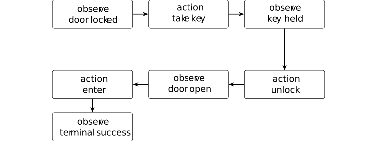
Let \(H_0=(\text {door locked})\). After action \(A_0=\text {take key}\), the environment returns \(O_1=\text {key held}\), so \(H_1=(H_0,A_0,O_1)\). Repeating the same update with unlock and door open, then choosing \(A_2=\text {enter}\), produces \(O_3=\text {terminal success}\) and \(H_3=(H_2,A_2,O_3)\). No later observation is available to an earlier action choice.
The alternating action--observation interface is the finite-history form of the agent setup in [kaelbling1998planning, Section 2]. The trace checks chronology and termination; uncertain state, partial observability, and language-valued actions lie beyond this deterministic instance.
Example 1.5.13. Token generation as a stopped environment interaction [ftip-0027]AGENTDRAFTED
Example 1.5.13. Token generation as a stopped environment interaction [ftip-0027]AGENTDRAFTED
A prefix tree represents token emission as a finite interaction stopped either by an end token or by a hard length cap.
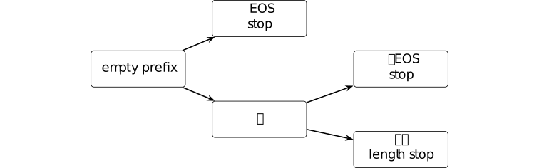
Take vocabulary \(\{a,\mathtt {EOS}\}\). The terminal histories are an immediate end token, an end token after \(a\), and a length-capped history \(aa\). Their probabilities are products of the conditional token laws and sum to one. The last history terminates because the declared maximum length is reached, not because the policy emitted \(\mathtt {EOS}\).
The causal token product is given in [phuong2022formal, Section 3]. The finite representation distinguishes two stopping mechanisms. Token steps remain distinct from tool calls, and unbounded generation is outside the construction.
Remark 1.5.14. The induced law of a stopped interaction [ftip-0028]AGENTDRAFTED
Remark 1.5.14. The induced law of a stopped interaction [ftip-0028]AGENTDRAFTED
Sutton and Barto's agent--environment interface in [sutton2018reinforcement, sec. 3.1] supplies alternating states, actions, and rewards. Kaelbling et al. separate hidden state and public observation in [kaelbling1998planning, Section 2]. A stopped interaction is determined by its initial law, transition--observation kernel, policy, and public stopping rule.
The induced interaction law uses four independently declared objects: the initial law \(\rho _0\) in Definition 1.5.2, the environment kernels \(K_t\) in Definition 1.5.3, the policy \(\pi _t\) in Definition 1.5.7, and the stopping rule in Definition 1.5.8. On finite spaces, the probability of a length-\(n\) trajectory before applying its stopping indicator factors as \[ \rho _0(s_0,o_0) \prod _{t=0}^{n-1} \pi _t(a_t\mid h_t) K_t(s_{t+1},o_{t+1}\mid s_t,a_t). \] The event \(\{\tau _{\mathrm {stop}}=n\}\) selects the stopped trajectories.
This factorization supports later expectations, likelihood ratios, and off-policy reuse. It also exposes an identifiability limit: an outcome distribution by itself generally does not reveal which of the initial law, environment, policy, or stopping rule changed.
2. Post-training, alignment, and feedback [ftip-00JA]AGENTDRAFTED
2. Post-training, alignment, and feedback [ftip-00JA]AGENTDRAFTED
Post-training procedures differ in the information they receive and the updates they permit. Demonstrations, preferences, rewards, verifiers, and environment interactions impose different conditions on the resulting policy.
The chapter moves from demonstrations and preferences to reward-based updates, then to training through tool interaction and replay. The agent-state analysis complements these parameter-changing procedures by examining the contexts, memories and computation an agent retains around its models.
2.1. Fine-tuning [ftip-006P]AGENTDRAFTED
2.1. Fine-tuning [ftip-006P]AGENTDRAFTED
Fine-tuning continues parameter optimization from a pretrained artifact. The term names a relation between an initial checkpoint, training records, an objective, and an update process. It does not by itself specify instruction data, preference feedback, or reinforcement learning.
Definition 2.1.1. Fine-tuning run [ftip-006Q]AGENTDRAFTED
Definition 2.1.1. Fine-tuning run [ftip-006Q]AGENTDRAFTED
Given the base artifact \(M_0=(\tau ,\delta ,\mathsf {cfg},\theta _K,\mathsf {num})\) from Definition 1.3.21, a fine-tuning run declares training records, a finite update count \(J\geq 0\), a loss \(L_{\rm ft}\), gradient estimators \(g_j^{\rm ft}\), optimizer states \(s_j^{\rm ft}\), and update specifications \((U_j,\eta _j^{\rm ft})\). It starts from \(\theta ^{\rm ft}_0=\theta _K\).
For each \(j=0,\ldots ,J-1\), the update is
\[ (\theta ^{\rm ft}_{j+1},s^{\rm ft}_{j+1}) =U_j\left (\theta ^{\rm ft}_j,s^{\rm ft}_j, g_j^{\rm ft},\eta _j^{\rm ft}\right ). \]Its output artifact replaces \(\theta _K\) by the final \(\theta ^{\rm ft}_J\). Any change to the tokenizer, architecture configuration, numerical convention, or other artifact field must be stated separately. Fine-tuning is not identified with one loss or data type.
Definition 2.1.2. Supervised fine-tuning in InstructGPT [ouyang2022training, Section 3.5 and Appendix C.1] [ftip-006H]AGENTDRAFTED
Definition 2.1.2. Supervised fine-tuning in InstructGPT [ouyang2022training, Section 3.5 and Appendix C.1] [ftip-006H]AGENTDRAFTED
In the cited pipeline, supervised fine-tuning (SFT) starts from a pretrained GPT-3 checkpoint and updates it by supervised learning on labeler demonstrations. The resulting policy supplies the starting and reference policy for later stages.
Appendix C.1 reports optimization choices for that construction. It does not define a universal mask, weighting rule, or fine-tuning protocol.
Remark 2.1.3. Fine-tuning objectives and supervised instances [ftip-006R]AGENTDRAFTED
Remark 2.1.3. Fine-tuning objectives and supervised instances [ftip-006R]AGENTDRAFTED
Wei et al. train on instruction-expressed task mixtures in [wei2022finetuned, Section 2 and Figure 2]. Ouyang et al. fine-tune on labeler demonstrations in [ouyang2022training, Section 3.5 and Appendix C.1]. The proposed continued-optimization interface in Definition 2.1.1 includes these concrete supervised instances.
Neither cited source defines fine-tuning as one universal objective. A concrete run must state its records, loss and normalization, optimizer, stopping rule, and trainable parameters. Instruction tuning later specializes the records to instruction--response demonstrations.
2.2. Instruction tuning [ftip-0029]AGENTDRAFTED
2.2. Instruction tuning [ftip-0029]AGENTDRAFTED
Instruction tuning uses demonstrations to connect the continuation law of a pretrained language model with requests written as instructions. The objects in this section separate the mathematical training record, its provenance, the reported collection procedure, and the loss used to update the model.
Notation 2.2.1. Prompts, responses, demonstrations, and loss masks [ftip-002A]AGENTDRAFTED
Notation 2.2.1. Prompts, responses, demonstrations, and loss masks [ftip-002A]AGENTDRAFTED
Let \(\mathcal X_{\mathrm {pr}}\) be the prompt space. For each prompt \(x\in \mathcal X_{\mathrm {pr}}\), let \(\mathcal Y(x)\subseteq \mathcal V^*\) be the set of finite token responses permitted by the training format. We write \(y=(y_1,\ldots ,y_{|y|})\in \mathcal Y(x)\) and \(y_{<t}=(y_1,\ldots ,y_{t-1})\).
A demonstration is denoted \(z=(x,y,\omega )\), where \(\omega \) is its provenance record. A finite multiset of demonstrations is denoted \(D_{\mathrm {sft}}\). For each response position, a loss mask \(m_t(z)\in \{0,1\}\) records whether the token contributes to the supervised objective, and a nonnegative weight \(w_t(z)\) records its declared normalization. Prompt tokens are conditioning context and lie outside the response-position domains of \(m_t(z)\) and \(w_t(z)\).
Definition 2.2.2. Prompt serializer [ftip-006V]AGENTDRAFTED
Definition 2.2.2. Prompt serializer [ftip-006V]AGENTDRAFTED
Using the prompt space of Notation 2.2.1, a prompt serializer is a declared map \[ s_{\mathrm {pr}}:\mathcal X_{\mathrm {pr}}\longrightarrow \mathcal V^*. \] For token strings \(u,v\in \mathcal V^*\), write \(u\mathbin {\Vert }v\) for their concatenation. A response token \(y_t\) is therefore predicted from the token prefix \(s_{\mathrm {pr}}(x)\mathbin {\Vert }y_{<t}\).
The serializer fixes system text, role markers, separators, and any other prompt-side control tokens. Changing it changes the conditional examples seen by the language model even when the abstract prompts and responses are unchanged.
Remark 2.2.3. Why instruction data require serialization [ftip-006W]AGENTDRAFTED
Remark 2.2.3. Why instruction data require serialization [ftip-006W]AGENTDRAFTED
The next-token law in Definition 1.2.8 accepts token prefixes, whereas an instruction dataset may store structured prompts. The proposed serializer in Definition 2.2.2 maps between those types. Ouyang et al. describe SFT on labeler demonstrations in [ouyang2022training, Section 3.5 and Appendix C.1]; their training account supplies a concrete pipeline rather than a universal serializer.
A reproducible objective must retain the serializer revision with the tokenizer and loss mask. Otherwise two runs can share an abstract dataset name while optimizing different token sequences.
Definition 2.2.4. Instruction tuning [wei2022finetuned, Section 2 and Figure 2] [ftip-002B]AGENTDRAFTED
Definition 2.2.4. Instruction tuning [wei2022finetuned, Section 2 and Figure 2] [ftip-002B]AGENTDRAFTED
Instruction tuning fine-tunes a pretrained language model on a mixture of tasks whose examples are expressed through natural-language instructions and corresponding target outputs. The task description and any input are placed in the prompt; the target output supplies the continuation to be learned.
The construction changes the model parameters by supervised learning. It does not require a learned reward model, preference comparisons, or interaction with an environment.
Definition 2.2.5. Demonstration record [ftip-002C]AGENTDRAFTED
Definition 2.2.5. Demonstration record [ftip-002C]AGENTDRAFTED
Using the notation of Notation 2.2.1, a demonstration record is a triple
\[ z=(x,y,\omega ), \qquad x\in \mathcal X_{\mathrm {pr}},\quad y\in \mathcal Y(x), \]where \(\omega \) identifies the declared producer of \(y\), the collection or generation procedure, and any selection rule applied before the record entered \(D_{\mathrm {sft}}\). The response is a training target; its presence in the data does not assert that it is uniquely correct or preferred to every alternative.
Remark 2.2.6. Demonstration and teacher provenance [ftip-002D]AGENTDRAFTED
Remark 2.2.6. Demonstration and teacher provenance [ftip-002D]AGENTDRAFTED
The provenance field \(\omega \) distinguishes a demonstration from the process that supplied it. Ouyang et al. collect labeler-written demonstrations in [ouyang2022training, §§3.2, 3.4]. Wei et al. permit a broader task mixture in [wei2022finetuned, §2; Fig. 2].
Human writers, stronger teacher models, filtered self-generations, and programmatically produced targets give different information to the learner. Claims about sample efficiency or capability acquisition must therefore state which producer and selection rule were available.
Definition 2.2.7. Labeler demonstration collection [ouyang2022training, Sections 3.2 and 3.4] [ftip-002E]AGENTDRAFTED
Definition 2.2.7. Labeler demonstration collection [ouyang2022training, Sections 3.2 and 3.4] [ftip-002E]AGENTDRAFTED
In the InstructGPT data-collection procedure, a labeler receives a prompt and writes a desired response. The resulting prompt--response pair enters the demonstration data used by the supervised fine-tuning stage. Prompts come from the declared API and labeler-written sources, and the paper records filtering and labeler-selection procedures.
This construction specifies a human demonstration channel. It is distinct from the later comparison channel, in which a labeler ranks model-generated responses rather than writing the target response.
Definition 2.2.8. Supervised fine-tuning objective [ftip-002F]AGENTDRAFTED
Definition 2.2.8. Supervised fine-tuning objective [ftip-002F]AGENTDRAFTED
For the language-model policy \(\pi _\theta \) and the notation of Notation 2.2.1, a masked supervised fine-tuning (SFT) objective has the form
\[ L_{\mathrm {sft}}(\theta ) =-\sum _{z=(x,y,\omega )\in D_{\mathrm {sft}}} \sum _{t=1}^{|y|}w_t(z)m_t(z) \log \pi _\theta \left (y_t\mid s_{\mathrm {pr}}(x)\mathbin {\Vert }y_{<t}\right ), \]where the nonnegative weights satisfy \(\sum _{z\in D_{\mathrm {sft}}}\sum _{t=1}^{|y|}w_t(z)m_t(z)=1\). The response index \(t\) does not range over serialized prompt tokens. Minimizing this objective increases conditional likelihood on the selected target tokens. The weights and mask are local conventions and must be declared for each implementation.
Convention 2.2.9. Response-token normalization [ftip-002G]AGENTDRAFTED
Convention 2.2.9. Response-token normalization [ftip-002G]AGENTDRAFTED
For a finite demonstration multiset, define the number of selected response tokens by
\[ N_{\mathrm {resp}} =\sum _{z=(x,y,\omega )\in D_{\mathrm {sft}}} \sum _{t=1}^{|y|}m_t(z). \]When \(N_{\mathrm {resp}}>0\), response-token normalization sets \(w_t(z)=N_{\mathrm {resp}}^{-1}\) at every selected position. Each selected token then has equal weight in \(L_{\mathrm {sft}}\). Equal weighting of records or prompts is a different convention because response lengths vary.
The training account alone does not determine this normalization. Any comparison of losses or gradients must retain the mask and normalization that produced them.
Example 2.2.10. Response-only supervision on one instruction record [ftip-002H]AGENTDRAFTED
Example 2.2.10. Response-only supervision on one instruction record [ftip-002H]AGENTDRAFTED
Two instruction positions provide conditioning context but lie outside the response-loss index set. The loss is taken on the two generated tokens.

Declare \(\pi (r_1\mid u_1,u_2)=1/2\) and \(\pi (r_2\mid u_1,u_2,r_1)=1/4\). The instruction tokens are not indexed by the response mask. With mask one on each displayed response token, the sum and mean are \[ L_{\rm sum}=-\log \tfrac 12-\log \tfrac 14=\log 8, \qquad L_{\rm mean}=\tfrac 12\log 8\approx 1.040. \]
The supervised objective in Definition 2.2.8 and the causal factorization in Definition 1.2.9 specialize to the displayed token strip. Its mask is a local choice on response positions; other instruction-tuning implementations may supervise a different subset of response tokens or declare a larger loss domain explicitly.
Remark 2.2.11. What instruction tuning changes and leaves open [ftip-002I]AGENTDRAFTED
Remark 2.2.11. What instruction tuning changes and leaves open [ftip-002I]AGENTDRAFTED
Instruction tuning changes conditional likelihood under a declared demonstration distribution. It can teach response format, task interpretation, and behavior represented by the targets, but the training loss alone does not identify which of those effects caused an independent evaluation gain.
Ouyang et al. report supervised fine-tuning and its optimization settings in [ouyang2022training, Section 3.5 and Appendix C.1]. They do not define the exact mask and weighting convention displayed in Definition 2.2.8; those choices remain part of the declared objective.
The stage also leaves several questions open. A demonstration does not compare its target with alternatives, a teacher may transmit errors or hidden information, and low loss on the collected prompts need not imply transfer to a new task law. Preference acquisition introduces a different observation: which response a judge selected from a displayed pair.
2.3. Preference acquisition and reward modeling [ftip-002J]AGENTDRAFTED
2.3. Preference acquisition and reward modeling [ftip-002J]AGENTDRAFTED
Preference data records a judge's choice between displayed alternatives. Reward modeling adds a statistical representation of those choices. This section keeps the acquisition procedure, observation law, score model, and validation law separate so that a scalar predictor is not mistaken for the preferences it was fitted to represent.
Notation 2.3.1. Comparison queries, judges, and response pairs [ftip-002K]AGENTDRAFTED
Notation 2.3.1. Comparison queries, judges, and response pairs [ftip-002K]AGENTDRAFTED
Use the prompt and response spaces from Notation 2.2.1. A comparison query is a displayed triple \(c=(x,y^0,y^1)\) with \(y^0,y^1\in \mathcal Y(x)\). Let \(\mathcal J\) be the declared judge population, and let \(j\in \mathcal J\) identify the human, model, or rule that returns a comparison label \(b_{\mathrm {pref}}\in \{0,1\}\).
When \(b_{\mathrm {pref}}=1\), write \(y^+=y^1\) and \(y^-=y^0\); when \(b_{\mathrm {pref}}=0\), reverse those names. Thus \(y^+\) means selected in this observation, not objectively or uniquely best. The acquisition mechanism may also record a tie, abstention, or invalid comparison, but those outcomes must use an enlarged label space rather than being silently forced into \(\{0,1\}\).
Definition 2.3.2. Pairwise comparison observation [ftip-002L]AGENTDRAFTED
Definition 2.3.2. Pairwise comparison observation [ftip-002L]AGENTDRAFTED
Restrict attention to a comparison for which the judge selects one displayed alternative rather than reporting indifference or incomparability. For a query \(c=(x,y^0,y^1)\) and a judge \(j\), a pairwise comparison observation is the displayed pair together with the judge's selected alternative. In winner--loser notation it is recorded as
\[ o=(x,y^+,y^-,j). \]The observation reports a choice made under the declared presentation and query procedure. It does not by itself provide a numerical reward, a complete ranking of responses, or a judgment about alternatives that were not shown.
Definition 2.3.3. Preference query selection [christiano2017deep, Section 2.2.4] [ftip-002M]AGENTDRAFTED
Definition 2.3.3. Preference query selection [christiano2017deep, Section 2.2.4] [ftip-002M]AGENTDRAFTED
Preference learning may choose which trajectory segments or responses to show to a judge rather than sampling every pair uniformly. The query-selection procedure assigns candidate comparisons a priority derived from the current reward-model ensemble and requests labels for selected pairs.
Because selection depends on the current model and candidate pool, the resulting comparison data reflect an acquisition policy. Active selection can concentrate labels on uncertain pairs, but it does not make the collected comparisons representative of an undeclared target population.
Remark 2.3.4. Preference acquisition and judge provenance [ftip-002N]AGENTDRAFTED
Remark 2.3.4. Preference acquisition and judge provenance [ftip-002N]AGENTDRAFTED
A preference observation depends on the query presented and the judge who evaluates it. Concrete elicitation procedures include [christiano2017deep, Sections 2.2.2 and 2.2.4] and the language-model comparison pipeline of [ouyang2022training, Sections 3.2 and 3.4].
The response generator, pair-selection rule, presentation order, judge population, and aggregation rule can each change the observed law. A later sample-complexity or population claim must condition on those choices rather than treating comparison labels as an unqualified source of ground truth.
Definition 2.3.5. Preference data law [ftip-002O]AGENTDRAFTED
Definition 2.3.5. Preference data law [ftip-002O]AGENTDRAFTED
A preference data law \(\mathcal D_{\mathrm {pref}}\) is a probability law on pairwise comparison observations \(o=(x,y^+,y^-,j)\) from Definition 2.3.2. It includes the randomness of prompt selection, response generation, pair selection, judge selection, and the judge's reported label.
A finite training multiset \(D_{\mathrm {pref}}=(o_1,\ldots ,o_N)\) is sampled or adaptively collected under that law and its acquisition history. When queries are adaptive, the records need not be independent or identically distributed.
Definition 2.3.6. Scalar reward-model score [ouyang2022training, Section 3.5 and Appendix C.2] [ftip-002P]AGENTDRAFTED
Definition 2.3.6. Scalar reward-model score [ouyang2022training, Section 3.5 and Appendix C.2] [ftip-002P]AGENTDRAFTED
A scalar reward model is a parameterized function
\[ r_\phi :\{(x,y):x\in \mathcal X_{\mathrm {pr}},\ y\in \mathcal Y(x)\} \longrightarrow \mathbb R, \]whose score is fitted from comparison observations. The score orders or weights responses for a specified training procedure; it is not automatically the independent utility of the response. Ouyang et al. initialize the model from the supervised policy and replace its language-model head with a scalar output for this stage.
Definition 2.3.7. Bradley--Terry comparison law [bradley1952rank, Page 325, equation (1)] [ftip-002Q]AGENTDRAFTED
Definition 2.3.7. Bradley--Terry comparison law [bradley1952rank, Page 325, equation (1)] [ftip-002Q]AGENTDRAFTED
Given scalar scores for two alternatives, the Bradley--Terry comparison law assigns the probability
\[ \Pr _\phi (y^+\succ y^-\mid x) =\frac {\exp r_\phi (x,y^+)} {\exp r_\phi (x,y^+)+\exp r_\phi (x,y^-)} =\sigma \left (r_\phi (x,y^+)-r_\phi (x,y^-)\right ), \]where \(\sigma (a)=(1+\exp (-a))^{-1}\). Conditioning the scores on a language-model prompt is the contextual specialization used in modern reward modeling; see also [rafailov2023direct, Section 3, equation (1)].
Definition 2.3.8. Pairwise reward-model loss [ouyang2022training, Section 3.5, equation (1), and Appendix C.2] [ftip-002R]AGENTDRAFTED
Definition 2.3.8. Pairwise reward-model loss [ouyang2022training, Section 3.5, equation (1), and Appendix C.2] [ftip-002R]AGENTDRAFTED
For comparison observations sampled from \(\mathcal D_{\mathrm {pref}}\), the pairwise reward-model loss is
\[ L_{\mathrm {rm}}(\phi ) =\mathbb E_{(x,y^+,y^-,j)\sim \mathcal D_{\mathrm {pref}}} \left [-\log \sigma \left ( r_\phi (x,y^+)-r_\phi (x,y^-) \right )\right ]. \]The empirical objective replaces the expectation by a declared weighting of the collected comparisons. It fits score differences under the Bradley--Terry law of Definition 2.3.7; it does not observe an absolute reward target for either response.
Remark 2.3.9. Representability, non-identifiability, and heterogeneous preferences [ftip-002S]AGENTDRAFTED
Remark 2.3.9. Representability, non-identifiability, and heterogeneous preferences [ftip-002S]AGENTDRAFTED
Fitting a Bradley--Terry predictor is an assumption about representation, not a consequence of observing comparisons. Cyclic choices, context effects, and mixtures of judges can fail to agree with one shared scalar ordering.
Even within the model, scores are not identified absolutely: replacing \(r_\phi (x,y)\) by \(r_\phi (x,y)+c(x)\) leaves every pairwise probability and the loss unchanged. Ouyang et al. give one normalization in [ouyang2022training, §3.5; App. C.2]. Other uses must state their own normalization, judge population, and validation law.
Example 2.3.10. A Bradley--Terry comparison calculation [ftip-002T]AGENTDRAFTED
Example 2.3.10. A Bradley--Terry comparison calculation [ftip-002T]AGENTDRAFTED
A declared difference between two reward scores maps to one Bradley--Terry preference probability.

Under the Bradley--Terry link, \[ \Pr (y^+\succ y^-\mid x) =\frac {\exp r(y^+)}{\exp r(y^+)+\exp r(y^-)} =\sigma (2-0.5) =\sigma (1.5)\approx 0.8176. \] Reversing the pair gives probability \(1-0.8176=0.1824\).
The fixed scores instantiate Definition 2.3.7 and determine the displayed probability. Whether one scalar reward can represent every judge is a separate modeling question.
Definition 2.3.11. Reward-model validation law [ftip-002U]AGENTDRAFTED
Definition 2.3.11. Reward-model validation law [ftip-002U]AGENTDRAFTED
A reward-model validation law \(\mathcal D_{\mathrm {rm}}^{\mathrm {val}}\) is a held-out law on comparison observations used to evaluate the fitted score model rather than to update \(\phi \). A declared validation statistic may be Bradley--Terry log loss or the probability that \(r_\phi (x,y^+)>r_\phi (x,y^-)\).
The validation population and acquisition procedure are part of the quantity. Accuracy on comparisons drawn from the same collection process does not establish calibration under a new judge population or agreement with an independent task-success criterion.
Remark 2.3.12. Reward-model validation depends on its population [ftip-006O]AGENTDRAFTED
Remark 2.3.12. Reward-model validation depends on its population [ftip-006O]AGENTDRAFTED
Ouyang et al. hold out comparison data and report reward-model validation accuracy and loss in [ouyang2022training, Section 3.5 and Appendix C.2]. Representing the validation population by a probability law makes the estimand depend explicitly on the judge population and acquisition procedure.
This law belongs to reward-model validation. It is not the independent task evaluation used later to compare post-training protocols.
Example 2.3.13. Cyclic preferences that no scalar ordering represents [ftip-002V]AGENTDRAFTED
Example 2.3.13. Cyclic preferences that no scalar ordering represents [ftip-002V]AGENTDRAFTED
Three strict comparisons arranged in a directed cycle obstruct representation by a single scalar ordering.
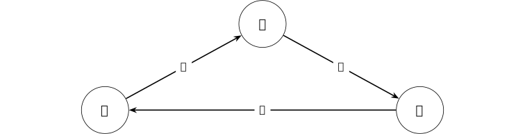
Declare \(A\succ B\), \(B\succ C\), and \(C\succ A\). If a scalar \(r\) represented all three comparisons by strict inequalities, then \[ r(A)>r(B)>r(C)>r(A), \] which implies \(r(A)>r(A)\), a contradiction. Thus no real-valued score can represent this cycle by ordinary greater-than.
Scalar pairwise reward modeling is used in [christiano2017deep, Section 2]; the finite cycle marks one assumption needed for that reduction. No empirical cycle is attributed to a particular dataset or population, and the obstruction concerns scalar orderings rather than all preference models.
2.4. Reinforcement-learning foundations [ftip-002W]AGENTDRAFTED
2.4. Reinforcement-learning foundations [ftip-002W]AGENTDRAFTED
Reinforcement learning updates a policy from rewards attached to sampled behavior. Before considering a particular alignment method, this section fixes the response-level episode, return, value, advantage, policy roles, and likelihood ratios used by policy-gradient objectives.
Notation 2.4.1. Reward, return, policy roles, value, advantage, and likelihood ratios [ftip-002X]AGENTDRAFTED
Notation 2.4.1. Reward, return, policy roles, value, advantage, and likelihood ratios [ftip-002X]AGENTDRAFTED
The ratio and policy-objective formulas in this section specialize the measurable policy interface of Definition 1.5.7 to a declared finite or countable discrete action space. Thus \(\pi (a\mid h)\) denotes probability mass, not an unspecified density. Whenever \(\log \pi _\theta (A_t\mid H_t)\) is displayed, its sampled mass is assumed positive.
For decision times \(t=0,\ldots ,N-1\), write \(\mathsf H_t:=H_t\) for the public history defined in Definition 1.5.5, \(A_t\) for its action, and \(R_{t+1}\in \mathbb R\) for the next reward. Let \(\gamma \in [0,1]\) be the discount factor and \(G_t\) the return from time \(t\).
Write \(\pi _b\) for the behavior policy that produced a stored action, \(\pi _\theta \) for the current trainable policy, and \(\pi _{\mathrm {ref}}\) for a fixed reference policy. Their value, action-value, and advantage functions are denoted \(V^\pi \), \(Q^\pi \), and \(A^\pi \); an estimated advantage is \(\widehat A_t\). The current-to-behavior likelihood ratio is denoted \(\rho _t(\theta )\).
In a response-level episode, \(\pi _\theta (y\mid x)\) abbreviates the completed-continuation probability \(P_\theta (y\mid s_{\mathrm {pr}}(x))\) of the response-task interface, using the declared prompt serializer; the same convention applies to \(\pi _b\) and \(\pi _{\mathrm {ref}}\). In an interactive episode these symbols instead denote the action laws on public histories defined in Definition 1.5.7.
Definition 2.4.2. Response-level episode [ouyang2022training, Section 3.5] [ftip-002Y]AGENTDRAFTED
Definition 2.4.2. Response-level episode [ouyang2022training, Section 3.5] [ftip-002Y]AGENTDRAFTED
In the response-level specialization used for language-model RLHF, a prompt \(x\) is the initial context, a complete response \(y\sim \pi _\theta (\mathord \cdot \mid x)\) is the sampled action, and a scalar score supplies the terminal reward. The episode terminates after that response.
This contextual-bandit view is sufficient for sequence-level reward-model training. Token generation may still be exposed as multiple policy decisions when an optimizer assigns token-level likelihood ratios or advantages. A later agentic setting also permits environment observations and tool actions between model responses.
Definition 2.4.3. Scalar reward [sutton2018reinforcement, Section 3.2] [ftip-002Z]AGENTDRAFTED
Definition 2.4.3. Scalar reward [sutton2018reinforcement, Section 3.2] [ftip-002Z]AGENTDRAFTED
A scalar reward \(R_{t+1}\in \mathbb R\) is the numerical signal received after action \(A_t\) and before the next decision. Its probabilistic law may depend on the current history, action, and environment transition.
Reward specifies the training objective of the reinforcement-learning problem. It need not equal an independent evaluator's utility, and a terminal reward need not identify which earlier action caused the outcome.
Definition 2.4.4. Return [sutton2018reinforcement, Section 3.3] [ftip-0030]AGENTDRAFTED
Definition 2.4.4. Return [sutton2018reinforcement, Section 3.3] [ftip-0030]AGENTDRAFTED
For an episode ending at time \(N\), the return from decision time \(t\) is
\[ G_t=\sum _{k=t}^{N-1}\gamma ^{k-t}R_{k+1}. \]When all intermediate rewards vanish, every return is determined by the terminal reward, up to discounting. Return is a random variable under the policy and environment law; its expectation defines value.
Definition 2.4.5. Value function [sutton2018reinforcement, Section 3.5] [ftip-0031]AGENTDRAFTED
Definition 2.4.5. Value function [sutton2018reinforcement, Section 3.5] [ftip-0031]AGENTDRAFTED
For a policy \(\pi \), the value function and action-value function are
\[ V^\pi (h)=\mathbb E_\pi [G_t\mid \mathsf H_t=h], \qquad Q^\pi (h,a)=\mathbb E_\pi [G_t\mid \mathsf H_t=h,A_t=a], \]whenever the conditional expectations exist. Both quantities depend on the reward, transition law, horizon, discount, and the policy followed after the conditioned decision.
Definition 2.4.6. Advantage function [schulman2016gae, Section 2] [ftip-0032]AGENTDRAFTED
Definition 2.4.6. Advantage function [schulman2016gae, Section 2] [ftip-0032]AGENTDRAFTED
For a policy \(\pi \), its advantage function is
\[ A^\pi (h,a)=Q^\pi (h,a)-V^\pi (h). \]The advantage compares an action with the policy's average continuation value at the same information state. Policy-gradient implementations replace it by an estimator \(\widehat A_t\); the estimator and the mathematical advantage are not interchangeable without assumptions on bias and variance.
Remark 2.4.7. Baselines and estimated credit [schulman2016gae, Sections 2--3] [ftip-0033]AGENTDRAFTED
Remark 2.4.7. Baselines and estimated credit [schulman2016gae, Sections 2--3] [ftip-0033]AGENTDRAFTED
Subtracting a baseline that does not depend on the sampled action can reduce the variance of a policy-gradient estimator without changing its expected gradient under the source conditions. A learned value function, a group mean, and a leave-one-out mean are different baselines and have different finite-data dependencies.
An estimated advantage may use sampled returns, bootstrapped values, or a mixture of both. Its error enters the update even when the likelihood-ratio calculation is exact.
Definition 2.4.8. Behavior, current, and reference policies [schulman2017proximal, Sections 2--3] [ftip-0034]AGENTDRAFTED
Definition 2.4.8. Behavior, current, and reference policies [schulman2017proximal, Sections 2--3] [ftip-0034]AGENTDRAFTED
The behavior policy \(\pi _b\) is the policy that generated a sampled action. The current policy \(\pi _\theta \) is the policy whose parameters are being optimized. Proximal policy optimization (PPO) collects a batch under an old policy and then compares candidate current policies with that data.
A reference policy \(\pi _{\mathrm {ref}}\) is instead held fixed to define a regularizer or preference objective; see [rafailov2023direct, Section 3, equation (3)]. It need not equal the behavior policy that generated a later rollout.
Definition 2.4.9. Likelihood ratio [schulman2017proximal, Section 2, equation (3)] [ftip-0035]AGENTDRAFTED
Definition 2.4.9. Likelihood ratio [schulman2017proximal, Section 2, equation (3)] [ftip-0035]AGENTDRAFTED
For an action \(A_t\) sampled from \(\pi _b\) at information state \(\mathsf H_t\), the current-to-behavior likelihood ratio is
\[ \rho _t(\theta ) =\frac {\pi _\theta (A_t\mid \mathsf H_t)}{\pi _b(A_t\mid \mathsf H_t)}. \]The ratio is defined on sampled actions for which \(\pi _b(A_t\mid \mathsf H_t)>0\). A bounded or clipped sampled ratio does not by itself control policy probabilities at unvisited histories.
Convention 2.4.10. Empirical sample average [ftip-006Z]AGENTDRAFTED
Convention 2.4.10. Empirical sample average [ftip-006Z]AGENTDRAFTED
For a nonempty finite index set \(I\) and real values \((Z_i)_{i\in I}\in \mathbb R^I\), write \[ \widehat {\mathbb E}_{i\in I}[Z_i] =\frac 1{|I|}\sum _{i\in I}Z_i. \] When the subscript is only \(t\), the index set is the declared collection of sampled decision times in the current batch.
PPO uses empirical expectation notation for its sampled surrogates; see Section 2, equations (1)--(2) of [schulman2017proximal]. The batch and its weighting must still be declared; the hat does not assert unbiasedness.
Definition 2.4.11. Policy-gradient surrogate [schulman2017proximal, Section 2, equations (1)--(2)] [ftip-0036]AGENTDRAFTED
Definition 2.4.11. Policy-gradient surrogate [schulman2017proximal, Section 2, equations (1)--(2)] [ftip-0036]AGENTDRAFTED
For samples collected under the declared behavior law and estimated advantages \(\widehat A_t\), the empirical policy-gradient surrogate is the following sample average:
\[ L^{\mathrm {PG}}(\theta ) =\widehat {\mathbb E}_t \left [\log \pi _\theta (A_t\mid \mathsf H_t)\,\widehat A_t\right ]. \]Its gradient is the familiar score-function estimator. The sampled states, actions, and advantage estimator are held fixed while differentiating this surrogate; changing the data-collection law defines a different estimator.
Example 2.4.12. Return and advantage on a three-step episode [ftip-0037]AGENTDRAFTED
Example 2.4.12. Return and advantage on a three-step episode [ftip-0037]AGENTDRAFTED
On a three-step episode, a discounted return and a baseline-relative advantage can be computed separately.

Take discount \(\gamma =1/2\). The return attached to the first action is \[ G_0=r_1+\gamma r_2+\gamma ^2 r_3 =0+\tfrac 12+\tfrac 14\cdot 2=1. \] If the declared baseline is \(V(s_0)=0.4\), then the corresponding advantage estimate is \(\widehat A_0=G_0-V(s_0)=0.6\).
The calculation instantiates the return and advantage in Definition 2.4.4 and Definition 2.4.6. It illustrates one baseline choice. Low variance and correct attribution of terminal reward to an internal decision require additional assumptions or evidence.
Remark 2.4.13. Delayed credit and estimator scope [ftip-0038]AGENTDRAFTED
Remark 2.4.13. Delayed credit and estimator scope [ftip-0038]AGENTDRAFTED
A terminal response score can be copied into returns for many token decisions, but that bookkeeping does not reveal which token caused the score.
Monte Carlo returns, learned values, generalized advantage estimation, and group-relative normalization make different bias, variance, and dependence choices. Any theorem about an update must name the estimator actually used, the behavior policy that supplied its samples, and the horizon over which its credit signal is propagated.
2.5. Alignment training [ftip-006S]AGENTDRAFTED
2.5. Alignment training [ftip-006S]AGENTDRAFTED
Alignment training describes a declared role for a parameter-changing procedure: it is intended to alter behavior relative to a stated criterion. The criterion and the evidence used during training must be named before the claim can be evaluated.
Definition 2.5.1. Alignment-training claim [ftip-006I]AGENTDRAFTED
Definition 2.5.1. Alignment-training claim [ftip-006I]AGENTDRAFTED
An alignment-training claim is a capability claim \((M_0,A,E_{\rm align},b)\) in the sense of Convention 1.1.1. The procedure \(A\) changes model parameters and declares its training observations, loss or reward, and update rule. The independently fixed criterion \(E_{\rm align}\) states the behavior relative to which the word ``alignment'' is used.
Calling a procedure alignment training does not assert that its criterion is complete or that optimizing its training signal improves an independent evaluation.
Remark 2.5.2. Alignment criteria across different training routes [ftip-006J]AGENTDRAFTED
Remark 2.5.2. Alignment criteria across different training routes [ftip-006J]AGENTDRAFTED
Ouyang et al. combine demonstrations, comparison-trained rewards, and PPO in [ouyang2022training, Sections 3.1--3.5]. Direct Preference Optimization replaces the learned-reward PPO stage with a preference loss in [rafailov2023direct, Section 4]. The broader alignment-training description is a proposed way to compare such routes; it does not identify their observations or objectives with one another.
The declared behavioral criterion is part of the claim, while the independent evaluation remains a separate object. Their agreement is an empirical or theoretical claim, not a consequence of the word alignment.
2.6. Reinforcement learning from human feedback and proximal policy optimization [ftip-0039]AGENTDRAFTED
2.6. Reinforcement learning from human feedback and proximal policy optimization [ftip-0039]AGENTDRAFTED
RLHF, short for reinforcement learning from human feedback, names a family of alignment-training pipelines. One influential pipeline fits a supervised policy, learns a reward model from comparisons, and then optimizes the policy against that reward while limiting movement from a reference policy. This section separates those pipeline choices from proximal policy optimization (PPO), the optimization method used in its final stage.
Definition 2.6.1. Language-model RLHF pipeline [ouyang2022training, Section 3.1, Figure 2, and Section 3.5] [ftip-003A]AGENTDRAFTED
Definition 2.6.1. Language-model RLHF pipeline [ouyang2022training, Section 3.1, Figure 2, and Section 3.5] [ftip-003A]AGENTDRAFTED
The InstructGPT pipeline first performs supervised fine-tuning on labeler demonstrations. It then samples response pairs, collects labeler rankings, and fits a scalar reward model. Finally, it samples responses from the trainable policy and applies PPO using the reward-model score together with a penalty relative to the supervised policy.
The three stages consume different records and optimize different losses. Calling their composition RLHF does not make supervised targets, pairwise preferences, learned rewards, and policy-gradient samples the same kind of feedback.
Remark 2.6.2. Reward modeling, alignment criteria, and policy optimization [ftip-003B]AGENTDRAFTED
Remark 2.6.2. Reward modeling, alignment criteria, and policy optimization [ftip-003B]AGENTDRAFTED
The RLHF pipeline makes three logically separate choices. The comparison data specify which judgments were observed; the reward model specifies how those observations are represented and generalized; the policy optimizer specifies how sampled actions change the model.
An alignment criterion lies outside this chain unless it is identified with the training reward by assumption. A reward model can predict its held-out comparisons while failing under policy-induced distribution shift, and PPO can increase the learned reward while independent utility stays fixed or falls.
Definition 2.6.3. Kullback--Leibler divergence [ftip-006X]AGENTDRAFTED
Definition 2.6.3. Kullback--Leibler divergence [ftip-006X]AGENTDRAFTED
For probability mass functions \(p\) and \(q\) on a finite or countable set \(\mathcal Y\), the Kullback--Leibler divergence of \(p\) relative to \(q\) is \[ D_{\mathrm {KL}}(p\Vert q) =\sum _{y\in \mathcal Y}p(y)\log \frac {p(y)}{q(y)}. \] We use \(0\log (0/q)=0\). If \(p(y)>0\) and \(q(y)=0\) for some \(y\), the value is \(+\infty \). On a countable set, the negative part of the displayed series is finite; a divergent positive part gives the value \(+\infty \). Since \(\mathcal V^*\) is countable, the definition applies to the response laws of Notation 2.2.1.
The order of the arguments matters. In particular, finiteness of the displayed forward divergence requires \(p\) to be absolutely continuous with respect to \(q\).
Remark 2.6.4. How the divergence enters alignment objectives [ftip-006Y]AGENTDRAFTED
Remark 2.6.4. How the divergence enters alignment objectives [ftip-006Y]AGENTDRAFTED
The KL-regularized reward objective appears as equation (3) in Section 3 of [rafailov2023direct]. Behavior-policy ratios, clipped ratios, and KL penalties enter alignment objectives for different purposes.
A coefficient multiplying \(D_{\mathrm {KL}}\) declares an optimization tradeoff. It is neither a guarantee that every sampled ratio is small nor an independent evaluation of the resulting policy.
Definition 2.6.5. KL-constrained RLHF objective [rafailov2023direct, Section 3, equation (3)] [ftip-003C]AGENTDRAFTED
Definition 2.6.5. KL-constrained RLHF objective [rafailov2023direct, Section 3, equation (3)] [ftip-003C]AGENTDRAFTED
Let \(\mu \) be a prompt law, \(r(x,y)\) a scalar reward, and \(\pi _{\mathrm {ref}}\) a fixed reference policy. For \(\beta >0\), the KL-regularized RLHF objective, using forward KL, is
\[ \max _{\pi } \mathbb E_{x\sim \mu ,\,y\sim \pi (\cdot \mid x)}[r(x,y)] -\beta \, \mathbb E_{x\sim \mu } \left [D_{\mathrm {KL}}\left ( \pi (\cdot \mid x)\Vert \pi _{\mathrm {ref}}(\cdot \mid x) \right )\right ]. \]The prompt law, reward, reference policy, and coefficient are part of the objective. The forward KL requires the optimized policy to be absolutely continuous with respect to the reference wherever the objective is finite.
Definition 2.6.6. KL-shaped PPO reward [ouyang2022training, Section 3.5, equation (2)] [ftip-003D]AGENTDRAFTED
Definition 2.6.6. KL-shaped PPO reward [ouyang2022training, Section 3.5, equation (2)] [ftip-003D]AGENTDRAFTED
For a prompt \(x\), sampled response \(y\), learned reward score \(r_\phi (x,y)\), and fixed reference policy \(\pi _{\mathrm {ref}}\), the sequence-level KL-shaped reward is
\[ R_{\mathrm {shape}}(x,y;\theta ) =r_\phi (x,y) -\beta \log \frac {\pi _\theta (y\mid x)} {\pi _{\mathrm {ref}}(y\mid x)}. \]Autoregressive factorization writes the logarithmic term as a sum of token-level log ratios. Ouyang et al. also mix a pretraining-gradient term into their reported PPO objective; that auxiliary term is separate from the shaped reward displayed here.
Definition 2.6.7. Generalized advantage estimator [schulman2016gae, Section 3, equations (10) and (16)] [ftip-003E]AGENTDRAFTED
Definition 2.6.7. Generalized advantage estimator [schulman2016gae, Section 3, equations (10) and (16)] [ftip-003E]AGENTDRAFTED
Given an approximate value function \(V\), with \(V(\mathsf H_N)=0\) at a terminal information state, define the temporal-difference residual
\[ \delta _t^V=R_{t+1}+\gamma V(\mathsf H_{t+1})-V(\mathsf H_t). \]For \(\lambda \in [0,1]\), the finite-episode generalized advantage estimator is
\[ \widehat A_t^{\mathrm {GAE}(\gamma ,\lambda )} =\sum _{l=0}^{N-t-1}(\gamma \lambda )^l\delta _{t+l}^V. \]The parameters \(\gamma \) and \(\lambda \) trade temporal reach against the variance and approximation error induced by bootstrapping. The estimator also depends on the fitted value function.
Definition 2.6.8. PPO clipped surrogate [schulman2017proximal, Section 3, equation (7)] [ftip-003F]AGENTDRAFTED
Definition 2.6.8. PPO clipped surrogate [schulman2017proximal, Section 3, equation (7)] [ftip-003F]AGENTDRAFTED
For a clipping parameter \(\epsilon _{\mathrm {clip}}\in (0,1)\), define \(\operatorname {clip}_{\epsilon _{\mathrm {clip}}}(u) =\min (1+\epsilon _{\mathrm {clip}},\max (1-\epsilon _{\mathrm {clip}},u))\). The PPO clipped surrogate is
\[ L^{\mathrm {CLIP}}(\theta ) =\widehat {\mathbb E}_t\left [ \min \left ( \rho _t(\theta )\widehat A_t, \operatorname {clip}_{\epsilon _{\mathrm {clip}}}(\rho _t(\theta )) \widehat A_t \right )\right ]. \]Clipping changes the sampled surrogate when the ratio moves outside the declared interval in a direction favored by the estimated advantage. It is not a hard bound on the KL divergence of the complete updated policy.
Definition 2.6.9. PPO value-and-entropy objective [schulman2017proximal, Section 5, equation (9)] [ftip-003G]AGENTDRAFTED
Definition 2.6.9. PPO value-and-entropy objective [schulman2017proximal, Section 5, equation (9)] [ftip-003G]AGENTDRAFTED
PPO implementations may optimize the combined sampled objective
\[ \widehat {\mathbb E}_t\left [ L_t^{\mathrm {CLIP}}(\theta ) -c_1\bigl (V_\theta (\mathsf H_t)-\widehat G_t\bigr )^2 +c_2\,\mathcal H\left (\pi _\theta (\cdot \mid \mathsf H_t)\right ) \right ], \]Here \(L_t^{\mathrm {CLIP}}\) is the per-sample integrand of the clipped surrogate in Definition 2.6.8, \(c_1,c_2\geq 0\), \(\widehat G_t\) is the declared value target, and, on the declared finite or countable discrete action set,
\[ \mathcal H(p)=-\sum _a p(a)\log p(a). \]The combined objective is used only when this nonnegative countable sum is finite, with \(0\log 0=0\). For a continuous action law, an implementation must instead declare a reference measure and the corresponding density-based entropy convention.
The value loss and entropy bonus change the shared-parameter update in addition to the clipped policy term. Their coefficients, target construction, and action space are part of the optimization method.
Definition 2.6.10. PPO rollout and minibatch update [schulman2017proximal, Section 5] [ftip-003H]AGENTDRAFTED
Definition 2.6.10. PPO rollout and minibatch update [schulman2017proximal, Section 5] [ftip-003H]AGENTDRAFTED
A PPO iteration collects a batch of trajectories under the behavior policy, computes returns or advantage estimates, and then performs several epochs of minibatch optimization on the same collected batch. The updated policy becomes the behavior policy for a later collection round.
The number of trajectories, epochs, minibatches, and optimizer steps governs how often one batch is reused. The clipped objective does not determine those protocol choices by itself.
Example 2.6.11. The PPO clipping cases for positive and negative advantage [ftip-003I]AGENTDRAFTED
Example 2.6.11. The PPO clipping cases for positive and negative advantage [ftip-003I]AGENTDRAFTED
Positive and negative advantages select different branches of the PPO clipped minimum.
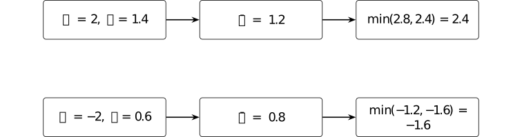
With \(\epsilon =0.2\), write \(\bar r=\operatorname {clip}(r,0.8,1.2)\) and \(L(r,A)=\min (rA,\bar rA)\). For positive advantage and \(r=1.4\), the gain is capped at \(2.4\). For negative advantage and \(r=0.6\), the clipped term \(-1.6\) is smaller than \(-1.2\), so the objective retains the penalty.
The pointwise surrogate comes from [schulman2017proximal, Section 3]. The two sign cases check only its arithmetic; they provide no monotone-improvement result for a neural policy or finite minibatch.
Example 2.6.12. The InstructGPT-style RLHF pipeline [ftip-003J]AGENTDRAFTED
Example 2.6.12. The InstructGPT-style RLHF pipeline [ftip-003J]AGENTDRAFTED
One prompt passes successively through supervised tuning, comparison-based reward modeling, and PPO in the InstructGPT-style RLHF pipeline.
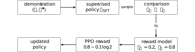
For the displayed illustrative prompt, suppose the comparison-trained reward model scores the preferred response by \(0.8\). If the candidate policy assigns it twice the probability assigned by the reference policy and the declared KL coefficient is \(\beta =0.1\), its shaped scalar is \[ 0.8-\beta \log \frac {\pi (y_B\mid x)} {\pi _{\rm ref}(y_B\mid x)} =0.8-0.1\log 2\approx 0.731. \]
The stage ordering is grounded in [ouyang2022training, Sections 3.1--3.5]; the numbers are a schematic calculation rather than reported InstructGPT hyperparameters. The diagram records the interface used in that pipeline. Other RLHF systems may order or replace the stages differently.
Remark 2.6.13. PPO is an optimizer, not an alignment definition [ftip-003K]AGENTDRAFTED
Remark 2.6.13. PPO is an optimizer, not an alignment definition [ftip-003K]AGENTDRAFTED
RLHF is a feedback-and-training pipeline; PPO is one optimizer used within that pipeline. PPO specifies a sampled update surrogate; it does not specify whose preferences are collected, what the reward means, or which independent behavior counts as aligned.
Changing the comparison population or reward model can change the alignment target while leaving PPO unchanged. Conversely, replacing PPO by another optimizer changes update geometry without necessarily changing the declared preference data or evaluation criterion.
2.7. Direct Preference Optimization [ftip-003L]AGENTDRAFTED
2.7. Direct Preference Optimization [ftip-003L]AGENTDRAFTED
Direct Preference Optimization rewrites a KL-regularized reward objective as a policy loss on preference pairs. The derivation proceeds through an optimal-policy identity, a reward--policy reparameterization, and a Bradley--Terry comparison probability. Keeping those steps separate makes its assumptions and its difference from reward-model PPO visible.
Notation 2.7.1. Temperature and reference-policy log ratios [ftip-003M]AGENTDRAFTED
Notation 2.7.1. Temperature and reference-policy log ratios [ftip-003M]AGENTDRAFTED
Let \(\beta >0\) be the KL coefficient, \(\pi _{\mathrm {ref}}\) a fixed reference policy, and \(\pi _\theta \) a trainable policy with support contained in that of the reference on the responses under study. Define the reference-relative log likelihood
\[ \ell _\theta (x,y) =\log \frac {\pi _\theta (y\mid x)}{\pi _{\mathrm {ref}}(y\mid x)} \]and, for a comparison observation, the paired difference
\[ \Delta _\theta (x,y^+,y^-) =\ell _\theta (x,y^+)-\ell _\theta (x,y^-). \]
Definition 2.7.2. Direct preference training stage [rafailov2023direct, Section 4] [ftip-003N]AGENTDRAFTED
Definition 2.7.2. Direct preference training stage [rafailov2023direct, Section 4] [ftip-003N]AGENTDRAFTED
Direct preference training starts from a fixed reference policy and a dataset of preferred and dispreferred responses. It evaluates a binary cross-entropy loss formed from the trainable policy's reference-relative log likelihoods and updates the policy directly.
This stage does not separately fit a scalar reward network, sample online rollouts for PPO, or train a value function. Its loss nevertheless comes from a particular reward-model and KL-regularized optimization derivation.
Definition 2.7.3. Optimal KL-regularized policy [rafailov2023direct, Section 4, equation (4)] [ftip-003O]AGENTDRAFTED
Definition 2.7.3. Optimal KL-regularized policy [rafailov2023direct, Section 4, equation (4)] [ftip-003O]AGENTDRAFTED
For a reward \(r(x,y)\), reference policy \(\pi _{\mathrm {ref}}\), and \(\beta >0\), the optimizer of the per-prompt KL-regularized reward objective has the form
\[ \pi _r(y\mid x) =\frac {1}{Z_r(x)}\, \pi _{\mathrm {ref}}(y\mid x) \exp \left (\frac {r(x,y)}{\beta }\right ), \]where
\[ Z_r(x)=\sum _y\pi _{\mathrm {ref}}(y\mid x) \exp \left (\frac {r(x,y)}{\beta }\right ) \]normalizes the policy on the response space. The identity assumes that the normalizer is finite and uses the same reference policy as the underlying objective.
Definition 2.7.4. Reward--policy reparameterization [rafailov2023direct, Section 4, equation (5)] [ftip-003P]AGENTDRAFTED
Definition 2.7.4. Reward--policy reparameterization [rafailov2023direct, Section 4, equation (5)] [ftip-003P]AGENTDRAFTED
Rearranging the optimal-policy identity of Definition 2.7.3 gives
\[ r(x,y) =\beta \log \frac {\pi _r(y\mid x)}{\pi _{\mathrm {ref}}(y\mid x)} +\beta \log Z_r(x). \]The final term depends on the prompt but not on the response. It cancels from pairwise reward differences, matching the additive non-identifiability of Bradley--Terry scores described in Remark 2.3.9.
Definition 2.7.5. Policy-ratio preference probability [rafailov2023direct, Section 4, equation (6)] [ftip-003Q]AGENTDRAFTED
Definition 2.7.5. Policy-ratio preference probability [rafailov2023direct, Section 4, equation (6)] [ftip-003Q]AGENTDRAFTED
Substituting the reward--policy reparameterization into the Bradley--Terry law yields
\[ \Pr _\theta (y^+\succ y^-\mid x) =\sigma \left (\beta \, \Delta _\theta (x,y^+,y^-) \right ), \]where \(\Delta _\theta \) is defined in Notation 2.7.1. The prompt-dependent normalizer cancels because the two responses share the same prompt.
Definition 2.7.6. Direct Preference Optimization loss [rafailov2023direct, Section 4, equation (7)] [ftip-003R]AGENTDRAFTED
Definition 2.7.6. Direct Preference Optimization loss [rafailov2023direct, Section 4, equation (7)] [ftip-003R]AGENTDRAFTED
For comparison observations from \(\mathcal D_{\mathrm {pref}}\), the Direct Preference Optimization loss is
\[ L_{\mathrm {DPO}}(\theta ) =-\mathbb E_{(x,y^+,y^-,j)\sim \mathcal D_{\mathrm {pref}}} \left [ \log \sigma \left (\beta \, \Delta _\theta (x,y^+,y^-) \right ) \right ]. \]The empirical loss is evaluated on a fixed comparison dataset. The temperature, reference policy, record weights, and handling of ties or abstentions are part of the training specification.
Example 2.7.7. A Direct Preference Optimization log-ratio calculation [ftip-003S]AGENTDRAFTED
Example 2.7.7. A Direct Preference Optimization log-ratio calculation [ftip-003S]AGENTDRAFTED
Four declared policy probabilities determine the log-ratio margin in one DPO loss term.

Let \(\pi _\theta (y^+\mid x)=0.6\), \(\pi _{\rm ref}(y^+\mid x)=0.3\), \(\pi _\theta (y^-\mid x)=0.2\), and \(\pi _{\rm ref}(y^-\mid x)=0.4\). With \(\beta =1/2\), the DPO logit is \[ z=\beta \left [\log 2-\log (1/2)\right ] =\tfrac 12\log 4=\log 2. \] Hence \(\sigma (z)=2/3\) and the one-pair negative log-likelihood is \(-\log \sigma (z)=\log (3/2)\approx 0.405\).
Substitution into Equation (7) of [rafailov2023direct, Section 4] verifies one loss term. Consistency of the pairwise data, suitability of the reference policy, and improvement in independent utility are separate questions.
Remark 2.7.8. Assumptions behind the DPO derivation [rafailov2023direct, Section 4 and Appendix A.1--A.2] [ftip-003T]AGENTDRAFTED
Remark 2.7.8. Assumptions behind the DPO derivation [rafailov2023direct, Section 4 and Appendix A.1--A.2] [ftip-003T]AGENTDRAFTED
The derivation uses a fixed reference policy, a finite KL-regularized optimum, and a Bradley--Terry model for pairwise preferences. The relevant policy probabilities must be positive wherever their logarithmic ratios are evaluated.
The algebra eliminates the prompt-dependent reward offset, not every source of reward-model misspecification. Heterogeneous or nontransitive preferences, adaptive data collection, support mismatch, and finite-sample optimization remain separate questions.
Remark 2.7.9. How DPO differs from reward-model PPO [rafailov2023direct, Sections 3--4] [ftip-003U]AGENTDRAFTED
Remark 2.7.9. How DPO differs from reward-model PPO [rafailov2023direct, Sections 3--4] [ftip-003U]AGENTDRAFTED
DPO optimizes a policy directly on a fixed preference dataset. Reward-model PPO instead fits an explicit scalar reward predictor, generates policy rollouts, estimates advantages, and applies a policy-gradient update. DPO therefore removes the separately represented reward and online PPO loop from that training stage.
The methods still share ingredients: comparison data, a reference policy, a KL coefficient or temperature, and assumptions connecting comparisons with latent reward. Neither method defines preference optimization in general, and their data and compute requirements are not causally interchangeable.
2.8. Outcome and process feedback [ftip-003V]AGENTDRAFTED
2.8. Outcome and process feedback [ftip-003V]AGENTDRAFTED
A completed response can receive one terminal judgment, while its intermediate steps can receive separate judgments. These feedback structures support different credit assignments. They must also be distinguished from signals that are actually available online before later steps are observed.
Definition 2.8.1. Outcome-supervised reward model [lightman2023verify, Section 2.5, ``Outcome-supervised reward models''] [ftip-003W]AGENTDRAFTED
Definition 2.8.1. Outcome-supervised reward model [lightman2023verify, Section 2.5, ``Outcome-supervised reward models''] [ftip-003W]AGENTDRAFTED
An outcome-supervised reward model assigns a score to a complete response and is trained from labels attached to the final outcome. For a prompt \(x\) and completed response \(y\), write its score as
\[ r_{\mathrm {out},\phi }(x,y)\in \mathbb R. \]The training label states whether the completed solution reaches the declared outcome. It need not identify the first invalid step or distinguish a sound derivation from an answer reached for an unsound reason.
Definition 2.8.2. Process-supervised reward model [lightman2023verify, Section 2.6, ``Process-supervised reward models''] [ftip-003X]AGENTDRAFTED
Definition 2.8.2. Process-supervised reward model [lightman2023verify, Section 2.6, ``Process-supervised reward models''] [ftip-003X]AGENTDRAFTED
Suppose a response is segmented into reasoning steps \(y=(s_1,\ldots ,s_m)\). A process-supervised reward model produces a score for each declared prefix,
\[ r_{\mathrm {proc},\phi }(x,s_{\leq k})\in \mathbb R, \qquad 1\leq k\leq m, \]and is fitted from step-level labels. The segmentation rule and label semantics are part of the supervision: a score after step \(k\) need not be a decomposition of an outcome score for the whole response.
Remark 2.8.3. Terminal and intermediate supervision [lightman2023verify, Sections 2.5--2.6] [ftip-003Y]AGENTDRAFTED
Remark 2.8.3. Terminal and intermediate supervision [lightman2023verify, Sections 2.5--2.6] [ftip-003Y]AGENTDRAFTED
Outcome supervision uses one completed-response label, whereas process supervision supplies labels at declared intermediate steps. The latter can localize feedback, but it also requires a segmentation, a step-labeling criterion, and additional annotations.
Neither label type is automatically causal credit. A process label may be assigned after a reviewer has seen the whole response, and a terminal outcome may be predicted reliably from an early prefix without identifying which action should change.
Definition 2.8.4. Online measurable feedback [ftip-003Z]AGENTDRAFTED
Definition 2.8.4. Online measurable feedback [ftip-003Z]AGENTDRAFTED
Let \(\mathcal F_t\) be the sigma-algebra generated by the public history \(\mathsf H_t\) available through decision time \(t\). A feedback variable \(Z_t\) is online measurable at time \(t\) when it is \(\mathcal F_t\)-measurable and is delivered before the protocol chooses its next action.
A label computed only after observing a later action or terminal outcome is not online measurable at the earlier time, even if it is subsequently attached to that earlier prefix in the training data.
Remark 2.8.5. Label timing and non-anticipating feedback [ftip-0040]AGENTDRAFTED
Remark 2.8.5. Label timing and non-anticipating feedback [ftip-0040]AGENTDRAFTED
The index attached to a label does not determine when its information becomes available. The process-supervision construction in [lightman2023verify, Section 2.6] supplies step-indexed training labels, but it does not require every such label to be available while the response is being generated.
This distinction determines which interventions are admissible. An online agent may act on currently measurable feedback; an offline learner may use a post-hoc label for a past prefix; a causal claim needs assumptions connecting either signal to the consequences of the earlier action.
Example 2.8.6. Terminal and process labels on the same four-step trace [ftip-0041]AGENTDRAFTED
Example 2.8.6. Terminal and process labels on the same four-step trace [ftip-0041]AGENTDRAFTED
A four-step arithmetic trace can receive a correct terminal label while retaining an incorrect intermediate process label.

The final answer \(19\) is correct, so outcome supervision supplies \(f_{\rm out}=1\). The declared process labels are \((f_1,f_2,f_3,f_4)=(1,1,0,1)\) and expose the corrected arithmetic error at step three. The labels are attached to the displayed prefixes, which remain unchanged by those annotations.
The two supervision regimes follow the outcome- and process-supervised reward-model constructions in [lightman2023verify, the outcome- and process-supervised reward-model subsections]. The two observations are thereby separated. Noise-free labels and a general policy advantage for process supervision are not consequences of the finite trace.
2.9. Reinforcement learning with verifiable rewards [ftip-0042]AGENTDRAFTED
2.9. Reinforcement learning with verifiable rewards [ftip-0042]AGENTDRAFTED
Reinforcement learning with verifiable rewards replaces or supplements a learned judge with a declared check of the generated result. Contemporary methods differ in their verifier, sampling law, advantage estimator, clipping, normalization, and treatment of length. This section defines those choices separately before they are assembled into a training protocol.
Notation 2.9.1. Verifiers, evidence, rollout groups, and group statistics [ftip-0043]AGENTDRAFTED
Notation 2.9.1. Verifiers, evidence, rollout groups, and group statistics [ftip-0043]AGENTDRAFTED
Let \(\mathcal E\) be an evidence space. Write \(\mathsf V\) for a declared verifier, \(e_{\mathrm {ver}}\in \mathcal E\) for its evidence, \(d_{\mathrm {ver}}\in \{0,1\}\) for its decision, and \(R_{\mathrm {ver}}\in \mathbb R\) for the reward derived from that result.
For a prompt \(x\) and group size \(g\geq 2\), write \(\mathbf Y_x=(Y^{(1)},\ldots ,Y^{(g)})\) for a rollout group sampled from the behavior policy. Let \(R_i\) be the reward of member \(i\), \(\bar R\) the group mean, \(S_R\) the group standard deviation, and \(\widehat A_i\) its group-relative advantage.
Definition 2.9.2. Reinforcement learning with verifiable rewards [lambert2024tulu3, Section 6, equations (7)--(8), and the paragraph following equation (8)] [ftip-0044]AGENTDRAFTED
Definition 2.9.2. Reinforcement learning with verifiable rewards [lambert2024tulu3, Section 6, equations (7)--(8), and the paragraph following equation (8)] [ftip-0044]AGENTDRAFTED
Reinforcement learning with verifiable rewards is a post-training method that samples responses from a language-model policy, computes rewards with a deterministic check of the response, and applies a reinforcement-learning update to increase expected checked reward, optionally with regularization to a reference policy.
In the cited construction, a correct response receives reward \(\alpha \) and an incorrect response receives \(0\). Equation (8) gives this two-valued form, and the paragraph immediately after it sets \(\alpha =10\). The checked predicate, reward scale, prompt law, rollout procedure, and policy optimizer remain separate parts of the method.
Remark 2.9.3. RLVR sampling, feedback, and update rules [ftip-0045]AGENTDRAFTED
Remark 2.9.3. RLVR sampling, feedback, and update rules [ftip-0045]AGENTDRAFTED
Concrete RLVR methods include the PPO-based construction in [lambert2024tulu3, Section 6], group relative policy optimization (GRPO) in [shao2024deepseekmath, Section 4.1], R1-Zero in [guo2025deepseek, Section 2.2], and Decoupled Clip and Dynamic sAmpling Policy Optimization (DAPO) in [yu2025dapo, Sections 2--3].
A proposed common description groups methods that acquire policy samples, evaluate a declared verifiable signal, assign credit, and update the policy. A specific claim must still name its verifier, group sampling, estimator, clipping, normalization, reference-policy treatment, and length rule.
Definition 2.9.4. Verifier correctness indicator [ftip-0046]AGENTDRAFTED
Definition 2.9.4. Verifier correctness indicator [ftip-0046]AGENTDRAFTED
For prompts and responses from Notation 2.2.1, a deterministic verifier correctness indicator is a declared map
\[ v:\{(x,y):x\in \mathcal X_{\mathrm {pr}},\ y\in \mathcal Y(x)\} \longrightarrow \{0,1\}, \]Here \(v(x,y)=1\) means that the response satisfies the checked predicate. The map includes the parsing and execution rules needed to reproduce the decision. A stochastic judge or learned reward model is a different feedback mechanism unless its randomness and decision procedure are separately exposed.
Definition 2.9.5. Verifier evidence [ftip-0047]AGENTDRAFTED
Definition 2.9.5. Verifier evidence [ftip-0047]AGENTDRAFTED
A verifier evidence record is a tuple
\[ e_{\mathrm {ver}}=(\iota _{\mathrm {ver}},x,y,o,d_{\mathrm {ver}}), \]where \(\iota _{\mathrm {ver}}\) identifies the verifier and its version, \(o\) is the reproducible output used by the check, and \(d_{\mathrm {ver}}\in \{0,1\}\) is the resulting decision. Examples of \(o\) include a parsed exact answer, a test log, or a proof-checker result.
The evidence record preserves how the decision was obtained. It does not assert that the checked predicate is complete for the task's independent success criterion.
Remark 2.9.6. A decision and reproducible evidence are distinct [ftip-0048]AGENTDRAFTED
Remark 2.9.6. A decision and reproducible evidence are distinct [ftip-0048]AGENTDRAFTED
The same correctness decision can arise from different parsers, tests, proof kernels, or failure modes. Tülu 3 uses a scaled two-valued reward \(\alpha \) or \(0\), with \(\alpha =10\), in [lambert2024tulu3, Section 6, equation (8), and the immediately following paragraph]; it does not identify that reward with a complete record of the checking procedure.
Evidence enables later audits of false positives, false negatives, version changes, and shortcut exploitation. Reproducibility of the check still does not establish that the checked predicate equals the intended capability.
Definition 2.9.7. Verifiable reward [lambert2024tulu3, Section 6, equation (8), and the immediately following paragraph] [ftip-0049]AGENTDRAFTED
Definition 2.9.7. Verifiable reward [lambert2024tulu3, Section 6, equation (8), and the immediately following paragraph] [ftip-0049]AGENTDRAFTED
Given a deterministic correctness indicator \(v\) and reward scale \(\alpha >0\), the verifiable reward in the cited construction is
\[ R_{\mathrm {ver}}(x,y)= \begin {cases} \alpha ,&v(x,y)=1,\\ 0,&v(x,y)=0. \end {cases} \]The paragraph after Equation (8) sets \(\alpha =10\). Another method may choose a different scale or combine several checked components, but that transformation is part of its reward design. A reward is verifiable relative to the implemented check, not relative to every property an independent evaluator may care about.
Remark 2.9.8. Rule, test, and proof evidence [ftip-004A]AGENTDRAFTED
Remark 2.9.8. Rule, test, and proof evidence [ftip-004A]AGENTDRAFTED
Rule evidence compares a parsed answer or format with a declared target, as in [guo2025deepseek, Section 2.2]. Test evidence executes a candidate in a sandbox and records test outcomes. Proof evidence submits a term to a specified checker and records acceptance or an error.
These routes expose different predicates and costs. A rule can ignore the derivation, a test suite can omit behavior, and a proof checker establishes only the proposition and trusted-kernel boundary it was given. Their rewards must not be merged without retaining which evidence source fired.
Definition 2.9.9. Rollout group [shao2024deepseekmath, Section 4.1.2] [ftip-004B]AGENTDRAFTED
Definition 2.9.9. Rollout group [shao2024deepseekmath, Section 4.1.2] [ftip-004B]AGENTDRAFTED
Fix a prompt \(x\), group size \(g\geq 2\), and behavior policy \(\pi _b\). A rollout group is the indexed family
\[ \mathbf Y_x=(Y^{(1)},\ldots ,Y^{(g)}), \qquad Y^{(i)}\sim \pi _b(\mathord \cdot \mid x). \]DeepSeekMath samples several outputs for the same prompt so their rewards can define a group-relative baseline. The producing policy, decoder, group size, and conditional sampling dependence are part of the rollout law.
Definition 2.9.10. Group mean and standard deviation [shao2024deepseekmath, Section 4.1.2] [ftip-004C]AGENTDRAFTED
Definition 2.9.10. Group mean and standard deviation [shao2024deepseekmath, Section 4.1.2] [ftip-004C]AGENTDRAFTED
For rollout-group rewards \(R_1,\ldots ,R_g\), define the group mean and group standard deviation by
\[ \bar R=\frac 1g\sum _{i=1}^g R_i, \qquad S_R=\operatorname {std}(R_1,\ldots ,R_g). \]Both statistics are prompt-local and depend on every member of the sampled group. The source leaves the standard-deviation divisor symbolic and does not add a numerical stabilizer. An implementation must state those conventions and its treatment of zero-variance groups.
Definition 2.9.11. Group-relative advantage [shao2024deepseekmath, Section 4.1.2] [ftip-004D]AGENTDRAFTED
Definition 2.9.11. Group-relative advantage [shao2024deepseekmath, Section 4.1.2] [ftip-004D]AGENTDRAFTED
When \(S_R>0\), the group-relative advantage of rollout member \(i\) is
\[ \widehat A_i=\frac {R_i-\bar R}{S_R}. \]The estimator compares responses sampled for the same prompt and does not require a learned value function. Its members are statistically coupled through \(\bar R\) and \(S_R\); it is not an independent estimate of the population advantage of each response.
Definition 2.9.12. Outcome-supervision GRPO [shao2024deepseekmath, Section 4.1.2] [ftip-004E]AGENTDRAFTED
Definition 2.9.12. Outcome-supervision GRPO [shao2024deepseekmath, Section 4.1.2] [ftip-004E]AGENTDRAFTED
Outcome-supervision GRPO samples a group of responses for one prompt, assigns each response an outcome reward, standardizes those rewards within the group, and uses the resulting group-relative advantage across the response's token log-likelihood terms.
The construction removes a separately learned critic but retains a behavior policy, likelihood ratios, a reference-policy term in the source formulation, and explicit normalization choices.
Definition 2.9.13. Process-supervision GRPO [shao2024deepseekmath, Section 4.1.3] [ftip-004F]AGENTDRAFTED
Definition 2.9.13. Process-supervision GRPO [shao2024deepseekmath, Section 4.1.3] [ftip-004F]AGENTDRAFTED
Process-supervision GRPO supplies rewards at declared reasoning steps and forms advantages from the subsequent step rewards assigned to each token. The policy objective therefore receives credit that can vary within one response rather than repeating one terminal outcome advantage at every token.
This construction requires a step segmentation and a process reward model. Its estimator is not obtained merely by relabeling an outcome-supervision rollout group.
Remark 2.9.14. GRPO variants and estimator conventions [shao2024deepseekmath, Section 4.1] [ftip-004G]AGENTDRAFTED
Remark 2.9.14. GRPO variants and estimator conventions [shao2024deepseekmath, Section 4.1] [ftip-004G]AGENTDRAFTED
GRPO names a family of group-relative policy updates rather than one fully determined estimator. Outcome and process supervision assign different reward structures. Implementations may also differ in token versus response normalization, KL terms, clipping intervals, importance weights, and treatment of groups with zero reward variance.
A result about one variant must retain its producing policy and all of those conventions. Sharing the group-relative baseline does not make the resulting gradients identical.
Definition 2.9.15. DAPO clip-higher [yu2025dapo, Section 3.1] [ftip-004H]AGENTDRAFTED
Definition 2.9.15. DAPO clip-higher [yu2025dapo, Section 3.1] [ftip-004H]AGENTDRAFTED
Clip-higher replaces the symmetric upper and lower PPO clipping widths by separate constants. It permits a larger upward likelihood-ratio movement for tokens with positive advantage while retaining a smaller lower-side interval.
The change alters which sampled terms are saturated by the surrogate. It does not impose a policy-wide trust region or guarantee preservation of low-probability actions.
Definition 2.9.16. Dynamic sampling [yu2025dapo, Section 3.2] [ftip-004I]AGENTDRAFTED
Definition 2.9.16. Dynamic sampling [yu2025dapo, Section 3.2] [ftip-004I]AGENTDRAFTED
DAPO dynamic sampling filters prompt groups whose sampled responses all receive the same reward and continues sampling until the training batch contains the declared number of groups with nonzero reward variation.
The intervention changes the distribution of prompts and rollouts entering the update. It can prevent zero-advantage groups from consuming an optimizer batch, but the retained batch is no longer an unconditioned sample from the original prompt law.
Definition 2.9.17. Token-level policy-gradient loss [yu2025dapo, Section 3.3] [ftip-004J]AGENTDRAFTED
Definition 2.9.17. Token-level policy-gradient loss [yu2025dapo, Section 3.3] [ftip-004J]AGENTDRAFTED
The token-level loss aggregates active token terms across the complete minibatch and divides by the number of active tokens. A longer response therefore contributes in proportion to its active token count rather than receiving the same total weight as every shorter response.
This normalization changes the empirical gradient even when the sampled responses, rewards, advantages, and likelihood ratios are unchanged. It must be distinguished from averaging a separately normalized loss over responses.
Definition 2.9.18. Overlong reward shaping [yu2025dapo, Section 3.4] [ftip-004K]AGENTDRAFTED
Definition 2.9.18. Overlong reward shaping [yu2025dapo, Section 3.4] [ftip-004K]AGENTDRAFTED
Overlong reward shaping introduces a soft penalty near the maximum response length before the hard truncation boundary. The penalty increases over a declared buffer region rather than assigning the same abrupt terminal penalty to every response that reaches the limit.
The construction changes both the reward value and which length-related behavior receives gradient. The maximum length, buffer width, and penalty schedule are part of the reward design.
Remark 2.9.19. These interventions change sampling and reward geometry [yu2025dapo, Sections 3.1--3.4] [ftip-004L]AGENTDRAFTED
Remark 2.9.19. These interventions change sampling and reward geometry [yu2025dapo, Sections 3.1--3.4] [ftip-004L]AGENTDRAFTED
Clip-higher changes the saturated region of the policy surrogate, dynamic sampling conditions which prompt groups enter a batch, token-level aggregation changes response-length weighting, and overlong shaping changes the reward near a truncation boundary. These are four different interventions.
An observed training improvement cannot be assigned to a generic ``algorithm'' without an ablation that holds the other sampling, estimator, reward, and compute choices fixed. The interventions also change which rollouts and gradients are observed, so their effects need not add linearly.
Example 2.9.20. One response-level RLVR round [ftip-004M]AGENTDRAFTED
Example 2.9.20. One response-level RLVR round [ftip-004M]AGENTDRAFTED
Three sampled responses pass through exact verification, group credit, and a proposed update in one finite RLVR round.
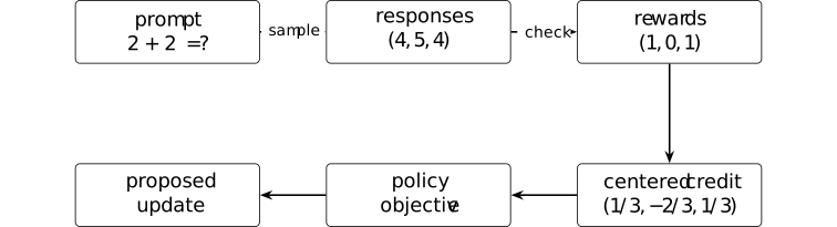
The exact-answer checker gives mean reward \(\bar r=2/3\). Using the declared unnormalized centered credit \(\widehat A_i=r_i-\bar r\) yields \((1/3,-2/3,1/3)\). An optimizer may use these numbers to propose a parameter change, but the tuple itself is not yet an accepted update.
The RLVR protocol is Definition 2.9.2. Its group-credit objects are Definition 2.9.9, Definition 2.9.10, and Definition 2.9.11. Together they specialize to this finite order of operations. Centered, unscaled credit and an exact-answer checker are local choices rather than requirements on other RLVR algorithms.
Example 2.9.21. Four rollout rewards, group advantages, and clipping [ftip-004N]AGENTDRAFTED
Example 2.9.21. Four rollout rewards, group advantages, and clipping [ftip-004N]AGENTDRAFTED
A rollout group is normalized to relative advantages and then passed to a clipped surrogate objective.

For a rollout group with rewards \(r_i\), form a group mean and scale and set \(\widehat A_i=(r_i-\bar r)/s\). For current-to-behaviour ratios \(\rho _i\) and clip interval \([1-\epsilon ,1+\epsilon ]\), define each pointwise term by
\[ \begin {aligned} \ell _i=\min \{&\rho _i\widehat A_i,\\ &\operatorname {clip}(\rho _i,1-\epsilon ,1+\epsilon )\widehat A_i\}. \end {aligned} \]The mean of the resulting terms is the group contribution to the update; its value depends on the sampled rewards, ratios, and clip width.
Group-relative normalization is grounded in [shao2024deepseekmath, Section 4.1], while clipping is grounded in [schulman2017proximal, Section 3]. The normalization convention and ratios must be declared by the training protocol; a positive surrogate mean alone gives no guarantee of improved held-out performance after an optimizer step.
2.10. Agentic post-training [ftip-004O]AGENTDRAFTED
2.10. Agentic post-training [ftip-004O]AGENTDRAFTED
Response-level training ends when a model emits an answer. Agentic post-training also trains decisions made after observations from tools or other external systems.
Definition 2.10.1. Action serializer [ftip-004P]AGENTDRAFTED
Definition 2.10.1. Action serializer [ftip-004P]AGENTDRAFTED
Fix the token vocabulary and strings of the tokenizer interface, and the action space \(\mathcal A\) from the declared interactive task realization. An action serializer is a pair of partial maps
\[ \operatorname {enc}:\mathcal A\rightharpoonup \mathcal V^*, \qquad \operatorname {dec}:\mathcal V^*\rightharpoonup \mathcal A. \]The encoder gives an action a textual representation. The decoder recognizes a completed representation and returns the executable action. A string outside the decoder's domain is malformed; it is not silently promoted to an environment action. For every action in the encoder's domain, the declared pair satisfies \(\operatorname {dec}(\operatorname {enc}(a))=a\).
Remark 2.10.2. Generated tokens and executable actions [ftip-004Q]AGENTDRAFTED
Remark 2.10.2. Generated tokens and executable actions [ftip-004Q]AGENTDRAFTED
An action serializer maps generated text to an executable action. Section 2 of ReAct: Synergizing reasoning and acting in language models[yao2023react] writes actions and observations in a textual trajectory. The proposed serializer interface in Definition 2.10.1 additionally distinguishes malformed calls, constrained grammars, and environment actions.
An improvement can therefore come from better reasoning, better serialization, or a more permissive parser. These are separate intervention coordinates.
Definition 2.10.3. tool interaction [yao2023react, Section 2] [ftip-004R]AGENTDRAFTED
Definition 2.10.3. tool interaction [yao2023react, Section 2] [ftip-004R]AGENTDRAFTED
A ReAct interaction alternates model-generated reasoning and actions with observations returned by an external interface. The observation is appended to the next model context, so subsequent actions may depend on earlier tool results.
A decoded action belongs to \(\mathcal A\) in the declared interactive task realization; the transition--observation kernel of Definition 1.5.3 returns the next observation. The cited construction does not by itself fix a sandbox, reward, or training algorithm.
Definition 2.10.4. Sandbox [ftip-004S]AGENTDRAFTED
Definition 2.10.4. Sandbox [ftip-004S]AGENTDRAFTED
Fix an interactive realization \(\mathsf {Env}_{\mathsf T}\) from the declared task interface, a measurable evidence space \(\mathcal E_{\rm box}\), and a cost dimension \(m\geq 1\). A sandbox specifies an allowed action set \(\mathcal A^{\rm box}_{\mathsf T}\subseteq \mathcal A_{\mathsf T}\) that is measurable, a cost bound \(b_{\rm box}\in \mathbb R_+^m\), and, for each \(x\in \mathcal X_{\mathsf T}\) and \(0\leq t<T_{\max }\), an execution kernel
\[ K_{t}^{\rm box,x}: \mathcal S_{\mathsf T}\times \mathcal A^{\rm box}_{\mathsf T} \rightsquigarrow \mathcal S_{\mathsf T}\times \mathcal O^{\rm obs}_{\mathsf T} \times \mathcal E_{\rm box}\times \mathbb R_+^m, \]It also specifies, for each \(x\in \mathcal X_{\mathsf T}\), a reset kernel
\[ \mathsf {Reset}^{x}_{\rm box}:\{\ast \}\rightsquigarrow \mathcal S_{\mathsf T}\times \mathcal O^{\rm obs}_{\mathsf T} \times \mathcal E_{\rm box}\times \mathbb R_+^m. \]For an allowed action, the state--observation marginal of \(K_t^{\rm box,x}\) is the kernel \(K_t^x\) in the task realization; the state--observation marginal of the reset kernel is \(\rho _0^x\). The remaining coordinates record reproducible evidence and a realized cost increment. An admitted stopped trajectory must have componentwise cumulative cost at most \(b_{\rm box}\).
The sandbox semantics include permissions, kernel and reset versions, evidence encoding, and cost accounting. A tool name or API schema alone does not determine these fields.
Remark 2.10.5. Sandbox restrictions and trajectory laws [ftip-004T]AGENTDRAFTED
Remark 2.10.5. Sandbox restrictions and trajectory laws [ftip-004T]AGENTDRAFTED
A sandbox restricts the environment through its executor, reset rules, permissions, and evidence. ReAct [yao2023react, Section 2] supplies the action--observation pattern. Software-agent systems surveyed in [wang2024agents, Section 2.3.2] add repositories, compilers, tests, and other digital tools. The combined sandbox interface is a proposed model of these choices.
Two protocols that share prompts but change reset or permission semantics need not induce the same trajectory law.
Definition 2.10.6. Agentic post-training state [ftip-004U]AGENTDRAFTED
Definition 2.10.6. Agentic post-training state [ftip-004U]AGENTDRAFTED
Let \(\mathcal M_{\rm exec}\) be the space of executable model artifacts, \(\mathcal Z_{\rm opt}\) the optimizer-state space, and \(\mathcal R_{\rm ag}\) a declared space of typed agentic round records. At training round \(n\), an agentic post-training state is a tuple \[ \Sigma _n=(M_n,s_n,\mathcal L_n) \in \mathcal M_{\rm exec}\times \mathcal Z_{\rm opt} \times \mathcal R_{\rm ag}^{n}, \] where \(M_n\) is the executable model artifact, \(s_n\) is the optimizer state, and \(\mathcal L_n=(r_0,\ldots ,r_{n-1})\) is an append-only training ledger.
The round-record schema records the task and instance draw, policy and inference stamp, environment version, stopped trajectory, feedback and credit outputs, update decision, proposed and committed next artifact and optimizer state, random seeds, operator versions, and realized cost vector. The tuple separates executable state from optimizer state and from evidence about how that state was reached.
Definition 2.10.7. One agentic post-training round [ftip-0073]AGENTDRAFTED
Definition 2.10.7. One agentic post-training round [ftip-0073]AGENTDRAFTED
At round \(n\), fix a task \(\mathsf T_n\), its law \(\mu _{\mathsf T_n}\), and a versioned interactive realization \(\mathsf {Env}^{\upsilon _n}_{\mathsf T_n}\). Let \(\mathcal I_{\rm art}\) and \(\mathcal I_{\rm inf}\) be declared identifier spaces. Let \(a_n\in \mathcal I_{\rm art}\) be an immutable content identifier resolving the artifact \(M_n\), and let \(\iota _n\in \mathcal I_{\rm inf}\) record all serializer, decoding, tool, and stopping settings. The policy--inference stamp \(\nu _n=(a_n,\iota _n)\in \mathcal I_{\rm art}\times \mathcal I_{\rm inf}\) resolves a non-anticipating policy \(\pi _n\). Let \(\Omega _n^{\rm task}\), \(\Omega _n^{\rm roll}\), \(\Omega _n^{\rm feed}\), \(\Omega _n^{\rm credit}\), and \(\Omega _n^{\rm update}\) be declared seed spaces. The rollout seed contains both policy-decoding and environment randomness. Write \(\Omega _n=\Omega _n^{\rm task}\times \Omega _n^{\rm roll}\times \Omega _n^{\rm feed}\times \Omega _n^{\rm credit}\times \Omega _n^{\rm update}\), and let \(\omega _n=(\omega _n^{\rm task},\omega _n^{\rm roll}, \omega _n^{\rm feed},\omega _n^{\rm credit},\omega _n^{\rm update})\) be sampled from a declared joint law on \(\Omega _n\). Write \(\mathcal Z_{\mathsf T_n}\) for the stopped trajectories admitted by the versioned realization.
For declared feedback and credit spaces \(\mathcal F_n\) and \(\mathcal G_n\), decision space \(\mathcal D_n=\{\mathsf {accept},\mathsf {reject}\}\), accounting dimension \(m\geq 1\), and exact implementation versions \(v_n^{\rm S}\), \(v_n^{\rm R}\), \(v_n^{\rm F}\), \(v_n^{\rm C}\), \(v_n^{\rm U}\), and \(v_n^{\rm A}\), the round specifies maps
\[ \begin {aligned} \mathsf S_n^{v_n^{\rm S}}&: \Omega _n^{\rm task}\longrightarrow \mathcal X_{\mathsf T_n},\\ \mathsf R_n^{v_n^{\rm R}}&: \mathcal X_{\mathsf T_n}\times \Omega _n^{\rm roll} \longrightarrow \mathcal Z_{\mathsf T_n},\\ \mathsf F_n^{v_n^{\rm F}}&: \mathcal X_{\mathsf T_n}\times \mathcal Z_{\mathsf T_n} \times \Omega _n^{\rm feed}\longrightarrow \mathcal F_n,\\ \mathsf C_n^{v_n^{\rm C}}&: \mathcal X_{\mathsf T_n}\times \mathcal Z_{\mathsf T_n} \times \mathcal F_n\times \Omega _n^{\rm credit} \longrightarrow \mathcal G_n,\\ \mathsf U_n^{v_n^{\rm U}}&: \mathcal M_{\rm exec}\times \mathcal Z_{\rm opt}\times \mathcal G_n \times \Omega _n^{\rm update} \longrightarrow \mathcal D_n\times \mathcal M_{\rm exec}\times \mathcal Z_{\rm opt},\\ \mathsf A_n^{v_n^{\rm A}}&: \mathcal M_{\rm exec}\times \mathcal Z_{\rm opt} \times \mathcal X_{\mathsf T_n}\times \mathcal Z_{\mathsf T_n}\\ &\quad {}\times \mathcal F_n\times \mathcal G_n\times \mathcal D_n\\ &\quad {}\times \mathcal M_{\rm exec}\times \mathcal Z_{\rm opt} \times \Omega _n\longrightarrow \mathbb R_+^m. \end {aligned} \]The accounting map receives the starting state, proposed state, decision, and realized seeds, so update work and rejected proposals remain observable in the cost record.
They produce
\[ \begin {aligned} X_n&=\mathsf S_n^{v_n^{\rm S}}(\omega _n^{\rm task}),\\ Z_n&=\mathsf R_n^{v_n^{\rm R}}(X_n,\omega _n^{\rm roll}),\\ F_n&=\mathsf F_n^{v_n^{\rm F}}(X_n,Z_n,\omega _n^{\rm feed}),\\ \Gamma _n&=\mathsf C_n^{v_n^{\rm C}} (X_n,Z_n,F_n,\omega _n^{\rm credit}),\\ (d_n,\widetilde M_{n+1},\widetilde s_{n+1}) &=\mathsf U_n^{v_n^{\rm U}} (M_n,s_n,\Gamma _n,\omega _n^{\rm update}),\\ c_n&=\mathsf A_n^{v_n^{\rm A}}( M_n,s_n,X_n,Z_n,F_n,\Gamma _n,d_n, \widetilde M_{n+1},\widetilde s_{n+1},\omega _n). \end {aligned} \]The task sampler pushes its seed law forward to \(\mu _{\mathsf T_n}\). Conditional on \(X_n\), the rollout sampler pushes its seed law forward to the interaction law of Remark 1.5.14 under \(\mathsf {Env}^{\upsilon _n}_{\mathsf T_n}\) and \(\pi _n\).
If \(d_n=\mathsf {accept}\), set \((M_{n+1},s_{n+1})=(\widetilde M_{n+1},\widetilde s_{n+1})\); if \(d_n=\mathsf {reject}\), set \((M_{n+1},s_{n+1})=(M_n,s_n)\). The realized cost \(c_n\) includes proposal work even after rejection. With \(v_n^{\rm ops}=(v_n^{\rm S},v_n^{\rm R},v_n^{\rm F},v_n^{\rm C}, v_n^{\rm U},v_n^{\rm A})\), append
\[ \begin {aligned} r_n={}&(\mathsf T_n,X_n,\nu _n,\upsilon _n,Z_n,F_n,\Gamma _n,d_n, \widetilde M_{n+1},\widetilde s_{n+1},M_{n+1},s_{n+1}, \omega _n,v_n^{\rm ops},c_n),\\ \mathcal L_{n+1}={}&\operatorname {append}(\mathcal L_n,r_n). \end {aligned} \]The record belongs to \(\mathcal R_{\rm ag}\) from Definition 2.10.6 and determines \(\Sigma _{n+1}\) without rewriting an earlier record.
Definition 2.10.8. Agentic post-training run [ftip-0074]AGENTDRAFTED
Definition 2.10.8. Agentic post-training run [ftip-0074]AGENTDRAFTED
An agentic post-training run fixes a finite round count \(N_{\rm ag}\geq 0\), an initial state \(\Sigma _0\), a fixed accounting dimension \(m\geq 1\), a componentwise budget \(b_{\rm ag}\in \mathbb R_+^m\), and the round specifications of Definition 2.10.7. Put \(\Omega _{\rm ag}=\prod _{n=0}^{N_{\rm ag}-1}\Omega _n\), using a singleton for the empty product. Once those specifications and their exact versions \(v_{\rm ag}\) are fixed, the run is the map
\[ \mathsf {Run}_{\Sigma _0,v_{\rm ag}}:\Omega _{\rm ag}\longrightarrow \mathcal M_{\rm exec}\times \mathcal R_{\rm ag}^{N_{\rm ag}} \times \mathbb R_+^m. \]Write a realized round-seed tuple as
\[ \omega _{\rm ag}=(\omega _0,\ldots ,\omega _{N_{\rm ag}-1}). \]The run recursively constructs \(\Sigma _1,\ldots ,\Sigma _{N_{\rm ag}}\); the seed tuple and state sequence are empty beyond \(\Sigma _0\) when \(N_{\rm ag}=0\). Its cumulative realized cost is \[ c_{\rm ag}=\sum _{n=0}^{N_{\rm ag}-1}c_n. \] The empty sum is \(0\in \mathbb R_+^m\) when \(N_{\rm ag}=0\). The map returns \((M_{N_{\rm ag}},\mathcal L_{N_{\rm ag}},c_{\rm ag})\). A run claiming the hard budget must declare a pre-admission or stopping rule that guarantees \(c_{\rm ag}\preceq b_{\rm ag}\).
The run declaration includes the task sampler, environments, serializers, rollout inference settings, feedback and credit maps, update maps, stopping rule, seed laws, implementation versions, and resource account. The round records retain every realized seed, version, decision, and cost. Leaving one of these fields implicit defines a family of runs rather than one reproducible intervention.
Remark 2.10.9. Post-training with intermediate observations [ftip-004X]AGENTDRAFTED
Remark 2.10.9. Post-training with intermediate observations [ftip-004X]AGENTDRAFTED
A proposed interactive extension of the response-level RLVR cycle in § 2.9 uses the environment of § 1.5 and the action boundary of Definition 2.10.1. It retains intermediate observations and environment state instead of treating a whole response as one indivisible action.
This change introduces new questions about partial observability, long-horizon credit, environment versioning, recovery after interruption, and the cost of external execution. It does not assert that multi-turn training is uniformly better than response-level training.
Example 2.10.10. A short code-agent trace with tool evidence [ftip-004V]AGENTDRAFTED
Example 2.10.10. A short code-agent trace with tool evidence [ftip-004V]AGENTDRAFTED
A failing test observation triggers a second edit, whose passing tool evidence determines the terminal result.
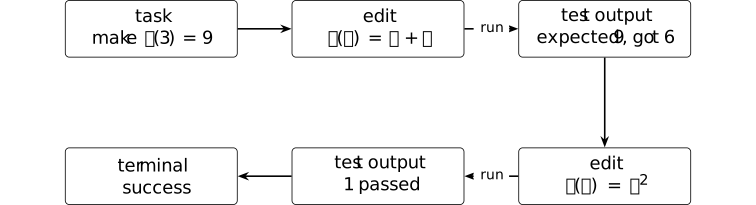
The public history records both edits and both test outputs. The first tool call returns the evidence string expected 9, got 6; the second returns exit status \(0\) and 1 passed. The success rule reads the second test result rather than the model's assertion that its edit is correct.
The action--observation alternation follows the tool-interleaving pattern in [yao2023react, Section 2]. The transparent sandbox interaction certifies only the displayed test result; completeness of the suite and satisfaction of unstated intent remain unverified.
Example 2.10.11. A DeepSeek-family resilient rollout and sandbox schematic [ftip-004W]AGENTDRAFTED
Example 2.10.11. A DeepSeek-family resilient rollout and sandbox schematic [ftip-004W]AGENTDRAFTED
Two coupled panels place resumable generation beside sandbox evidence in a single rollout record.
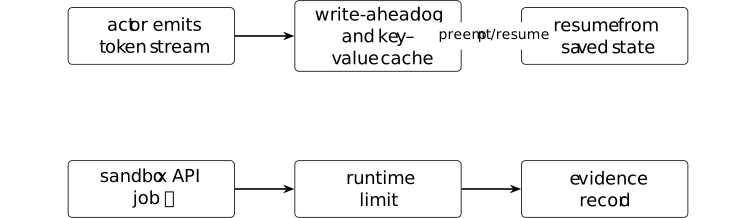
A write-ahead log and cached state allow a resumable rollout; a sandbox execution contributes a separately recorded evidence tuple. The two records should remain distinguishable when lifecycle cost is audited.
Token-granular write-ahead logging with key--value cache recovery and DeepSeek Elastic Compute (DSec), the report's named sandbox interface, are described in Sections 5.2.3 and 5.2.5 of the DeepSeek-V4 family report [⧉]. The cited sources do not establish that DeepSeek-V4-Flash-0731 used this job, resource limit, rollout schedule, or sandbox configuration.
2.11. Feedback, replay, and update control [ftip-004Y]AGENTDRAFTED
2.11. Feedback, replay, and update control [ftip-004Y]AGENTDRAFTED
Post-training systems often reuse historical trajectories. This section separates what happened during a rollout from quantities recomputed when that rollout is considered for another update.
Definition 2.11.1. Policy stamp [ftip-004Z]AGENTDRAFTED
Definition 2.11.1. Policy stamp [ftip-004Z]AGENTDRAFTED
A policy stamp \(\nu \) is a content-addressed description of an executable policy: model artifact, tokenizer, action serializer, decoding settings, and implementation revision. Resolving the stamp produces the action law \(\pi ^\nu (\,\cdot \mid \mathsf H_t)\) for every public history in its declared domain.
Two stamps are equal only when every component that may change the action law is equal. A display name or checkpoint step is therefore insufficient.
Remark 2.11.2. Behavior policies and executable-policy identity [ftip-0050]AGENTDRAFTED
Remark 2.11.2. Behavior policies and executable-policy identity [ftip-0050]AGENTDRAFTED
Off-policy methods distinguish the behavior and current policies, while language-model artifacts also depend on tokenization and decoding. Section 3 of When to stop reusing: Dynamic gradient gating for sample-efficient RLVR[miao2026when] records the behavior/current distinction. The additional artifact and implementation fields in the proposed policy stamp make the executable law reproducible.
The stamp identifies an executable law; it does not claim that two implementations with different stamps must behave differently on every task.
Definition 2.11.3. Immutable rollout record [ftip-0051]AGENTDRAFTED
Definition 2.11.3. Immutable rollout record [ftip-0051]AGENTDRAFTED
An immutable rollout record is a tuple
\[R=(q,\nu _b,\tau ,e),\]where \(q\) is the sampled task, \(\nu _b\) is the behavior-policy stamp, \(\tau \) is the stopped trajectory of Definition 1.5.9, and \(e\) is the verifier evidence of Definition 2.9.5. The tuple records facts fixed when the rollout finishes.
Current-policy likelihood ratios, clipping decisions, reuse counts, and acceptance decisions are excluded because they may change on a later update attempt.
Remark 2.11.4. A historical event is not an update attempt [ftip-0052]AGENTDRAFTED
Remark 2.11.4. A historical event is not an update attempt [ftip-0052]AGENTDRAFTED
An immutable historical record prevents an update attempt from rewriting the facts attached to its reused samples. The sample-reuse setup in [miao2026when, Section 3] retains behavior-policy rollouts while recomputing current-policy ratios. Dynamic Gradient Gating (DGG), defined in [miao2026when, Section 5 and Algorithm 1], is one such reuse protocol, while the complete immutable tuple is a proposed interface for such protocols.
Recorded facts and estimates recomputed for an attempted update are different objects; errors in the latter do not alter the former.
Definition 2.11.5. Feedback operator [ftip-0053]AGENTDRAFTED
Definition 2.11.5. Feedback operator [ftip-0053]AGENTDRAFTED
Let \(\mathcal R\) be the set of immutable rollout records and \(\mathcal F\) a typed set of feedback events. A feedback operator is a possibly randomized kernel
\[\mathsf {Feed}:\mathcal R\rightsquigarrow \mathcal F.\]A feedback event may contain an outcome score, step labels, a preference, or an abstention. Its type records which observations were available when it was produced.
Definition 2.11.6. Credit-assignment rule [ftip-0054]AGENTDRAFTED
Definition 2.11.6. Credit-assignment rule [ftip-0054]AGENTDRAFTED
Let \(R\) be a rollout record with \(\tau _{\rm stop}\) actions, and let \(f\) be its feedback event. A credit-assignment rule returns indexed training targets
\[\mathsf {Credit}(R,f)=(c_0,\ldots ,c_{\tau _{\rm stop}-1}).\]Each \(c_t\) is attached to an action or token position declared by the rule. It may be a return, an advantage estimate, a binary label, or a structured target. The rule is distinct from the feedback source that supplied \(f\).
Remark 2.11.7. Observed feedback and assigned credit [ftip-0055]AGENTDRAFTED
Remark 2.11.7. Observed feedback and assigned credit [ftip-0055]AGENTDRAFTED
Terminal returns, process labels, preference observations, and verifier rewards determine what information is observed. A credit rule determines where that information enters an objective. Treating them as separate inputs is a proposed common description of these different methods.
Separating the interfaces permits questions about delayed, noisy, or misallocated credit without changing the underlying evidence.
Definition 2.11.8. Replay pool [ftip-0056]AGENTDRAFTED
Definition 2.11.8. Replay pool [ftip-0056]AGENTDRAFTED
At update index \(n\), a replay pool \(\mathcal R_n\) is a finite multiset of immutable rollout records eligible for selection. Its management rule specifies insertion, eviction, and any partition by task or behavior stamp.
The pool is persistent state of the training protocol. It is not the minibatch selected for one update.
Definition 2.11.9. Attempt-local replay annotation [ftip-0057]AGENTDRAFTED
Definition 2.11.9. Attempt-local replay annotation [ftip-0057]AGENTDRAFTED
Selecting \(R\in \mathcal R_n\) under a current policy stamp \(\nu _n\) produces an attempt-local replay annotation
\[a_n(R)=(\nu _n,\rho ,\kappa ,m,u),\]where \(\rho \) is the declared collection of behavior/current likelihood ratios, \(\kappa \) records clipping status, \(m\) is the record age, and \(u\) is its prior reuse count. Every component is computed for this attempt and may change at the next one.
Remark 2.11.10. Replay selection and current-policy annotations [ftip-0058]AGENTDRAFTED
Remark 2.11.10. Replay selection and current-policy annotations [ftip-0058]AGENTDRAFTED
The proposed replay interface separates a persistent pool from annotations computed for an update attempt. DGG in [miao2026when, Section 3; Section 5 and Algorithm 1] recomputes policy ratios and a gradient diagnostic while reusing a rollout batch. Those quantities depend on the current policy and therefore belong to the attempted update rather than the historical record.
The split also exposes the cost of selecting, scoring, and rejecting reused records.
Example 2.11.11. Selecting a historical rollout under a current policy stamp [ftip-0059]AGENTDRAFTED
Example 2.11.11. Selecting a historical rollout under a current policy stamp [ftip-0059]AGENTDRAFTED
Reusing one historical rollout recomputes current-policy annotations without mutating the stored record.
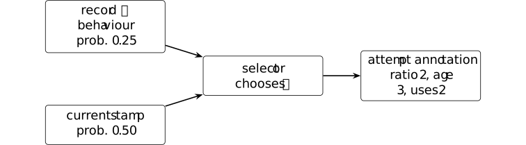
Let the stored record be \(R=(q,\nu _b,\tau ,e)\) and suppose its behaviour policy assigned the recorded action probability \(0.25\). Under the current stamp the same action has probability \(0.50\), so this attempt records importance ratio \(0.50/0.25=2\). Its age \(3\) and prior-use count \(2\) are also attempt-time metadata; none of these three values rewrites \(R\).
The behaviour/current-policy distinction is required by the reuse analysis in [miao2026when, Section 3]. The finite annotation makes provenance explicit. Statistical safety of ratio \(2\), age \(3\), or a second reuse is left undecided.
Definition 2.11.12. Update proposal [ftip-006C]AGENTDRAFTED
Definition 2.11.12. Update proposal [ftip-006C]AGENTDRAFTED
Given a current parameter--optimizer state \((\theta _n,z_n)\), selected records, their attempt annotations, and credit targets, an update proposal is a candidate next state
\[(\widetilde \theta _{n+1},\widetilde z_{n+1}, \delta _n^{\rm diag}).\]The diagnostic record \(\delta _n^{\rm diag}\) contains the quantities required by the declared acceptance rule. It is distinct from the accept--reject decision \(d_n\) recorded for the proposal. Constructing the proposal incurs update cost even if the proposal is later rejected.
Definition 2.11.13. dynamic gradient gate [miao2026when, Section 5 and Algorithm 1] [ftip-005A]AGENTDRAFTED
Definition 2.11.13. dynamic gradient gate [miao2026when, Section 5 and Algorithm 1] [ftip-005A]AGENTDRAFTED
Dynamic gradient gating computes the language-model-head gradient before the optimizer step. It compares the change in squared Frobenius norm with a trailing-window Z-score. When the score crosses its threshold after a reused update, the method discards that gradient and returns to fresh rollouts.
The gate is an empirical stopping rule for reuse. The source does not prove that its Z-score is a calibrated divergence test or a general safety certificate.
Remark 2.11.14. Rejected updates still consume computation [ftip-006D]AGENTDRAFTED
Remark 2.11.14. Rejected updates still consume computation [ftip-006D]AGENTDRAFTED
A gate may reject a computed gradient even though its computation has already consumed resources. The DGG definition in Definition 2.11.13 supplies the motivating pre-optimizer discard operation. Other protocols may inspect held-out loss, divergence, or resource limits.
The generic proposal interface does not transfer DGG's empirical detector to those other diagnostics. Each gate needs its own assumptions and calibration evidence.
Example 2.11.15. Two proposed updates under a DGG-style gate [ftip-005B]AGENTDRAFTED
Example 2.11.15. Two proposed updates under a DGG-style gate [ftip-005B]AGENTDRAFTED
Two candidate reused-gradient updates fall on opposite sides of a declared DGG-style gate.
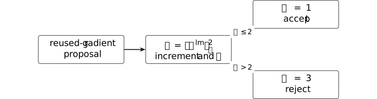
Declare a trailing-window increment mean \(\mu =1\), standard deviation \(s=0.5\), and toy threshold \(z_\star =2\). Proposal A has increment \(1.5\), so \(Z_A=(1.5-1)/0.5=1\) and is committed. Proposal B has increment \(2.5\), so \(Z_B=3\) and is rejected before an Adam transition. Rejection therefore leaves both parameters and optimizer moments unchanged in this protocol.
The monitored last-layer gradient energy, trailing-window Z-score, and pre-optimizer rejection order are modeled on [miao2026when, Section 5 and Algorithm 1]; the numeric threshold and window statistics above are locally declared. Acceptance is a reuse heuristic; it supplies neither a safety certificate nor a guarantee of improved independent evaluation.
Definition 2.11.16. checkpoint-trajectory extrapolation [chen2026lowrank, Sections 4 and 5.1] [ftip-0069]AGENTDRAFTED
Definition 2.11.16. checkpoint-trajectory extrapolation [chen2026lowrank, Sections 4 and 5.1] [ftip-0069]AGENTDRAFTED
NExt forms global and local parameter differences from saved low-rank adaptation (LoRA) checkpoints, approximates each matrix difference by leading singular factors, and trains a predictor on those representations to estimate a future difference. It adds a scaled predicted difference to a checkpoint; the reported experiments then resume RLVR updates.
The construction replaces some realized rollout-and-update steps with a learned parameter jump. It does not introduce a new verifier signal.
Remark 2.11.17. Trajectory compression and feedback acquisition [ftip-006A]AGENTDRAFTED
Remark 2.11.17. Trajectory compression and feedback acquisition [ftip-006A]AGENTDRAFTED
The NExt construction Low-rank optimization trajectories modeling for LLM RLVR acceleration[chen2026lowrank] motivates a distinction between following a predictable parameter path and acquiring information from new rollouts. Low-rank dominance of saved differences does not imply linear future motion, invariance across parameterizations, or preservation of optimizer state.
A cost comparison includes checkpoint storage, decomposition, predictor training, extrapolation, and recovery updates. Bounding independent-evaluation regret additionally requires stability assumptions connecting parameter forecasts to the evaluated outcome.
Example 2.11.18. A sign-invariant checkpoint-trajectory forecast [ftip-006B]AGENTDRAFTED
Example 2.11.18. A sign-invariant checkpoint-trajectory forecast [ftip-006B]AGENTDRAFTED
Leading rank-one projectors encode a checkpoint direction without inheriting the arbitrary signs of singular vectors.

For either singular-vector representation \((u,v)\) or \((-u,-v)\), the projectors \(P_u=uu^\top \) and \(P_v=vv^\top \) are unchanged. A trajectory forecaster can extrapolate the observed projector-aligned deltas to a next checkpoint, after which a measured recovery update can correct the forecast without changing the represented one-dimensional subspace.
The history-to-delta-to-recovery order is a toy illustration of NExt, described in [⧉]. NExt models signed singular value decomposition (SVD) factors rather than the projector construction used here. Accordingly, the calculation supplies neither a theorem about checkpoint trajectories nor evidence of capability acquisition.
3. Agent state, computation, and reliability [ftip-00JD]AGENTDRAFTED
3. Agent state, computation, and reliability [ftip-00JD]AGENTDRAFTED
An agent's behavior can change through persistent state, retained context and recursive execution even when its model weights are fixed. These mechanisms complement post-training, and their costs and retained artifacts belong to the same capability comparison.
The chapter begins with persistent state and lifecycle accounting, then examines dynamic computation and recursive harnesses. Failure modes and reliability protocols explain when an apparent gain can be trusted. Evaluation transport is developed with the independent evaluation framework that follows.
3.1. Persistent harness state and lifecycle-bounded inference [ftip-00C2]AGENTDRAFTED
3.1. Persistent harness state and lifecycle-bounded inference [ftip-00C2]AGENTDRAFTED
An executable model can remain fixed while a harness changes the context, available computation, retained memories, skills, subagent definitions, and evaluation policy around it. Those changes can alter later behavior and cost, but they are not weight training.
Distinguishing harness state from represented weights makes replay and descendant accounting precise, and exposes the effects of lossy summaries and contaminated refinement.
[karten2026prime] supplies operational records for persistent harness state. The Grothendieck-constant case study of [li2026longhorizon] supplies a long-horizon record in which compressed research state lost a caveat and a feasibility condition. Source observations remain empirical; the displayed finite results are proved here.
3.1.1. Fixed-weight harness adaptation [ftip-00C3]AGENTDRAFTED
3.1.1. Fixed-weight harness adaptation [ftip-00C3]AGENTDRAFTED
The executable model artifact, active context, explicitly managed computation, and persistent harness state are distinct parts of an agent. Replayability depends on the rule that materializes state from events, as well as the recorded inputs and execution versions.
Definition 3.1.1.1. Parameter, context, compute, and persistent state [ftip-00C4]AGENTDRAFTED
Definition 3.1.1.1. Parameter, context, compute, and persistent state [ftip-00C4]AGENTDRAFTED
Let \(\mathcal C_{\rm act}\) be an active-context space, \(\mathcal Z_{\rm man}\) an explicitly managed computation-state space, and \(\mathcal H_{\rm pers}\) a persistent harness-state space. A four-layer harness state is
\[ \Xi =(M,c,z,h)\in \mathcal M_{\rm exec}\times \mathcal C_{\rm act} \times \mathcal Z_{\rm man}\times \mathcal H_{\rm pers}. \]The coordinates are, respectively, the executable model artifact, the token-visible context, explicitly managed values or sessions, and state that can survive the present invocation. A transition may change any declared subset of these coordinates. A fixed-weight harness transition holds \(M\) fixed while changing one or more of \(c,z,h\).
Remark 3.1.1.2. State layers are access mechanisms, not capability levels [ftip-00C5]AGENTDRAFTED
Remark 3.1.1.2. State layers are access mechanisms, not capability levels [ftip-00C5]AGENTDRAFTED
Prime Agent Section 2.2 names model weights, active context, explicitly managed computation, and retained state as levels L0--L3, and describes the operations that move information between them [karten2026prime, Section 2.2]. The formulation in Definition 3.1.1.1 preserves that operational separation without treating the labels as an ordering of intelligence or capability.
Two runs with identical weights and different persistent state can induce different policies. That observation does not say that either run acquired a new circuit in the fixed artifact, and it does not compare their independently evaluated utility.
Definition 3.1.1.3. Versioned harness configuration [ftip-00C6]AGENTDRAFTED
Definition 3.1.1.3. Versioned harness configuration [ftip-00C6]AGENTDRAFTED
Let \(\mathcal I_{\rm har}\) be a content-identifier space. A versioned harness configuration is a finite record \(\kappa ^{\rm har}\in \mathcal I_{\rm har}\) that resolves the active-context assembly rule, managed-computation interface, tool permissions, session and message semantics, compaction policy, persistent-state schema, refinement policy, recovery rule, and implementation versions.
Together with a state \(\Xi \), the record resolves a non-anticipating harness policy. Changing one field produces a different declared intervention even when the executable model artifact is unchanged. The record does not include an evaluation binding; that is a separate record coordinate.
Definition 3.1.1.4. Persistent event stream [ftip-00C7]AGENTDRAFTED
Definition 3.1.1.4. Persistent event stream [ftip-00C7]AGENTDRAFTED
Fix a finite event alphabet \(\mathcal E_{\rm har}\). A persistent event stream of length \(n\) is
\[ L_n=(e_0,\ldots ,e_{n-1})\in \mathcal E_{\rm har}^{n}. \]The append operation is \(L_{n+1}=\operatorname {append}(L_n,e_n)\). Write \(L_i\preceq _{\rm pref}L_j\) when \(L_i\) is a prefix of \(L_j\). An append-only stream satisfies \(L_i\preceq _{\rm pref}L_j\) for every \(i\leq j\); branching creates distinct continuations with a common prefix rather than rewriting that prefix.
Events may record model or tool calls, messages, interventions, retries, verifier outcomes, harness edits, and resource use. The event schema and its exact version belong to the configuration of Definition 3.1.1.3.
Definition 3.1.1.5. Materialized harness state [ftip-00C8]AGENTDRAFTED
Definition 3.1.1.5. Materialized harness state [ftip-00C8]AGENTDRAFTED
Let \(\mathcal V_{\rm fold}\) be a space of fold versions. For each \(v\in \mathcal V_{\rm fold}\), fix a deterministic map
\[ F_v:\mathcal H_{\rm pers}\times \mathcal E_{\rm har} \longrightarrow \mathcal H_{\rm pers}. \]Given an initial persistent state \(h_0\), event stream \(L_n=(e_0,\ldots ,e_{n-1})\), and version sequence \(\boldsymbol v=(v_0,\ldots ,v_{n-1})\), its materialized harness state is obtained recursively by
\[ h_{i+1}=F_{v_i}(h_i,e_i),\qquad 0\leq i<n. \]The materialization record is the tuple \((h_0,L_n,\boldsymbol v,(F_v)_v)\). Omitting a version or the initial state defines a family of possible materializations, not one replayable state.
Theorem 3.1.1.6. Deterministic event folding gives replayable state [ftip-00C9]AGENTDRAFTED
Theorem 3.1.1.6. Deterministic event folding gives replayable state [ftip-00C9]AGENTDRAFTED
For a materialization record in Definition 3.1.1.5, replaying the same initial state, event sequence, version sequence, and fold maps produces the same state \(h_n\).
This finite result follows from the displayed hypotheses. It assumes exact equality of all recorded inputs and deterministic fold maps.
Proof.
At step zero both replays have state \(h_0\). If their states agree at
step \(i\), both apply the same function \(F_{v_i}\) to the same pair
\((h_i,e_i)\), so their states agree at step \(i+1\). Finite induction gives
equality at step \(n\).Proof.
Remark 3.1.1.7. Replayability is not correctness [ftip-00CA]AGENTDRAFTED
Remark 3.1.1.7. Replayability is not correctness [ftip-00CA]AGENTDRAFTED
The result in Theorem 3.1.1.6 is an identity about a declared transition system. It does not show that the event stream is complete, that an external process can be reconstructed, that the fold is faithful to the environment, or that the resulting state is useful or safe.
Prime Agent reports append-only events, versioned state, recovery, and rollback in Sections 2.2 and 2.5 [karten2026prime, Sections 2.2 and 2.5]. Those implementation claims motivate the event record; Theorem 3.1.1.6 proves the finite replay identity directly from the declared transition rule.
Example 3.1.1.8. One artifact and two harness policies [ftip-00CB]AGENTDRAFTED
Example 3.1.1.8. One artifact and two harness policies [ftip-00CB]AGENTDRAFTED
The same executable artifact can be paired with two persistent states and therefore two resolved harness policies. The harness state changes while the executable model remains fixed.
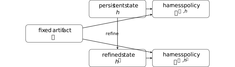
Different policies here establish only that harness state is an intervention coordinate. An independent evaluation is still required to compare their outcomes.
Remark 3.1.1.9. Fixed-weight self-improvement is not weight training [ftip-00CC]AGENTDRAFTED
Remark 3.1.1.9. Fixed-weight self-improvement is not weight training [ftip-00CC]AGENTDRAFTED
Prime Agent Section 2.5 uses the phrase ``self-improvement'' for execution evidence converted into persistent prompts, memories, skills, or subagent specifications while model weights remain fixed [karten2026prime, Section 2.5]. In the notation of Definition 3.1.1.1, this is a change to \(h\) with \(M\) held fixed.
The term therefore does not establish a change to the model artifact, a new learned circuit, or capability acquisition in the sense of Definition 1.1.5. It describes persistent harness adaptation.
3.1.2. Evaluation binding and lineage accounting [ftip-00CD]AGENTDRAFTED
3.1.2. Evaluation binding and lineage accounting [ftip-00CD]AGENTDRAFTED
A long-horizon score is attached to a configuration, not merely to a model name. Delegation also creates descendant work that must remain visible in the resource account. Reproducible evaluation therefore requires a specified configuration, and resource accounting includes the work of its descendants.
Definition 3.1.2.1. Evaluation configuration record [ftip-00CE]AGENTDRAFTED
Definition 3.1.2.1. Evaluation configuration record [ftip-00CE]AGENTDRAFTED
An evaluation configuration record is a finite record \(\mathfrak e\) that resolves the task and instance law, environment and tool interfaces, executable model artifact, serializer and inference policy, harness configuration, compaction and refinement policies, retry rule, completion gate, evaluator, seed law, and componentwise resource limits.
Together with the independent evaluation interface of Convention 4.1.1, the record determines the law of a stopped evaluation run and its realized cost vector. A reported score is the pair consisting of the statistic and the exact record \(\mathfrak e\); a scalar without its record is an under-specified family of measurements.
Remark 3.1.2.2. A harness comparison needs a declared configuration axis [ftip-00CF]AGENTDRAFTED
Remark 3.1.2.2. A harness comparison needs a declared configuration axis [ftip-00CF]AGENTDRAFTED
Section 2.6 of [karten2026prime] binds task and tool interfaces to model settings. Its evaluation configuration also records compaction, refinement, retry, completion, and resource policies. The record in Definition 3.1.2.1 is a proposed representation of those configuration choices.
To attribute a score difference to a harness coordinate, the comparison must hold the other coordinates fixed or model their changes explicitly. Two scores under different records \(\mathfrak e\) and \(\mathfrak e'\) can still be descriptively useful, but their difference does not isolate a causal harness effect.
Definition 3.1.2.3. Session lineage tree [ftip-00CG]AGENTDRAFTED
Definition 3.1.2.3. Session lineage tree [ftip-00CG]AGENTDRAFTED
A session lineage tree is a finite rooted directed tree \(\mathcal T=(V,E,r)\) whose edges point from a parent session to a directly spawned descendant. Each node \(v\in V\) carries an immutable session identifier, its resolved harness and inference stamps, a local event stream, and a local realized cost \(c_v\in \mathbb R_+^m\).
For a node \(v\), let \(\mathcal T_v\) be the induced subtree containing \(v\) and all its descendants. Distinct children of one node have disjoint node sets. Messages between branches are events in their local streams and do not merge their identities or costs.
Definition 3.1.2.4. Descendant-complete cost [ftip-00CH]AGENTDRAFTED
Definition 3.1.2.4. Descendant-complete cost [ftip-00CH]AGENTDRAFTED
For a session lineage tree Definition 3.1.2.3, its descendant-complete cost is the componentwise sum
\[ C_{\rm lin}(\mathcal T)=\sum _{v\in V}c_v\in \mathbb R_+^m. \]The local cost \(c_v\) contains only work assigned to node \(v\); a model or tool call is charged to exactly one node. The vector retains its declared units and embeds into the lifecycle account of Definition 4.1.5. A scalar price can be applied only after the vector is formed.
Theorem 3.1.2.5. Lineage cost is additive over disjoint child subtrees [ftip-00CI]AGENTDRAFTED
Theorem 3.1.2.5. Lineage cost is additive over disjoint child subtrees [ftip-00CI]AGENTDRAFTED
Let the root \(r\) of a finite lineage tree have children \(v_1,\ldots ,v_k\). Then
\[ C_{\rm lin}(\mathcal T)=c_r+ \sum _{j=1}^{k}C_{\rm lin}(\mathcal T_{v_j}). \]This finite accounting identity follows from assigning each local cost to exactly one node.
Proof.
The node set is the disjoint union of \(\{r\}\) and the node sets of
the child subtrees. Splitting the finite sum in
Definition 3.1.2.4 over that disjoint union gives the equality componentwise.Proof.
Definition 3.1.2.6. Budget-admissible continuation [ftip-00CJ]AGENTDRAFTED
Definition 3.1.2.6. Budget-admissible continuation [ftip-00CJ]AGENTDRAFTED
Fix a componentwise hard budget \(b\in \mathbb R_+^m\). After accumulated cost \(a\preceq b\), a proposed continuation has a declared worst-case cost bound \(\bar c\in \mathbb R_+^m\). It is budget-admissible when
\[ a+\bar c\preceq b. \]If admitted, the continuation must either stop within a realized cost \(c\preceq \bar c\) or report a contract violation. Rejected proposals may have a separately accounted proposal cost, which must already be included in \(a\) before the admission test.
Theorem 3.1.2.7. Budget admission preserves a hard componentwise bound [ftip-00CK]AGENTDRAFTED
Theorem 3.1.2.7. Budget admission preserves a hard componentwise bound [ftip-00CK]AGENTDRAFTED
Consider a finite sequence of continuations. Start from \(a_0\preceq b\). At step \(i\), admit only if \(a_i+\bar c_i\preceq b\), and require the realized cost to satisfy \(c_i\preceq \bar c_i\). With \(a_{i+1}=a_i+c_i\), every accumulated cost satisfies \(a_i\preceq b\).
This finite result is a contract theorem, not a prediction that a real executor respects its declared bound.
Proof.
The claim holds for \(a_0\). If \(a_i\preceq b\) and the next step is
admitted, then
\(a_{i+1}=a_i+c_i\preceq a_i+\bar c_i\preceq b\). If the step is rejected,
the accumulated cost is unchanged after its already-accounted proposal work.
Finite induction proves the claim.Proof.
Example 3.1.2.8. A finite delegated run and its lineage cost [ftip-00CL]AGENTDRAFTED
Example 3.1.2.8. A finite delegated run and its lineage cost [ftip-00CL]AGENTDRAFTED
Use two cost coordinates, such as output tokens and tool calls. The root delegates to two children, and one child delegates once more.
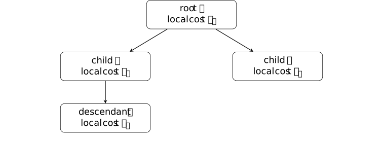
The cost of a child subtree is its local cost plus the costs of all descendants. Therefore
\[ C_{\rm lin}(\mathcal T)=c_r+C_{\rm lin}(\mathcal T_a)+C_{\rm lin}(\mathcal T_b). \]Charging only the root hides descendant work; charging a descendant again as a separate parent-local cost double counts it.
Remark 3.1.2.9. External benchmark points do not isolate a harness effect [ftip-00CM]AGENTDRAFTED
Remark 3.1.2.9. External benchmark points do not isolate a harness effect [ftip-00CM]AGENTDRAFTED
Prime Agent Section 3.1 places native-harness runs beside externally reported ARC-AGI-3 results and explicitly says the external points situate the curves rather than isolate a causal harness effect [karten2026prime, Section 3.1]. That is an empirical comparison under multiple evaluation records, not a matched estimate of one harness field.
A larger score can still be a valid record of the displayed configuration. It does not by itself establish that persistence caused the difference, that the model weights improved, or that the cost-adjusted potential of Definition 4.1.10 increased.
3.1.3. Research-state compaction and observability [ftip-00CN]AGENTDRAFTED
3.1.3. Research-state compaction and observability [ftip-00CN]AGENTDRAFTED
A research harness cannot place its complete archive into every model invocation. A summary can make distinct archives indistinguishable to later evaluators. The source record of a lost evaluator caveat illustrates how omitted information can affect subsequent research.
Definition 3.1.3.1. Active research state [ftip-00CO]AGENTDRAFTED
Definition 3.1.3.1. Active research state [ftip-00CO]AGENTDRAFTED
Let \(\mathcal A_{\rm res}\) be a space of complete research archives and \(\mathcal S_{\rm res}\) a space of bounded working summaries. Let \(\mathcal Q_{\rm claim}\) be a typed claim-ledger space and \(\mathcal G_{\rm res}\) a research-goal space. An active research state is
\[ R=(A,s,q,g)\in \mathcal A_{\rm res}\times \mathcal S_{\rm res} \times \mathcal Q_{\rm claim}\times \mathcal G_{\rm res}. \]The archive \(A\) may exceed the context budget. The summary \(s\) is the representation actually supplied to a new bounded session. The claim ledger \(q\) records declared statuses such as proved, numerically supported, conjectural, or heuristic. The goal \(g\) records the currently selected research direction.
Definition 3.1.3.2. Technical executor and research-judgment kernel [ftip-00CP]AGENTDRAFTED
Definition 3.1.3.2. Technical executor and research-judgment kernel [ftip-00CP]AGENTDRAFTED
Let \(\mathcal P_{\rm res}\) be a proposal space and \(\mathcal D_{\rm res}\) a finite research-decision space. A technical executor is a kernel that produces candidate calculations, experiments, lemmas, or implementations from the active summary and goal. A research-judgment kernel is
\[ J:\mathcal S_{\rm res}\times \mathcal Q_{\rm claim} \times \mathcal G_{\rm res}\times \mathcal P_{\rm res} \longrightarrow \Delta (\mathcal D_{\rm res}). \]The kernel chooses among actions such as continue, reframe, verify, merge, withdraw, or stop. It is typed separately from the executor because producing a technically valid local step and choosing the globally useful next step are different intervention coordinates.
Definition 3.1.3.3. Research-state summary operator [ftip-00CQ]AGENTDRAFTED
Definition 3.1.3.3. Research-state summary operator [ftip-00CQ]AGENTDRAFTED
A research-state summary operator is a declared map
\[ C:\mathcal A_{\rm res}\longrightarrow \mathcal S_{\rm res}. \]At a session boundary the harness supplies \(s=C(A)\). The operator may select, merge, compress, or omit archive content. Its input archive and exact version belong to the persistent event record. A stochastic summarizer is represented by adjoining its random seed to the archive coordinate, leaving \(C\) deterministic on the augmented input.
Definition 3.1.3.4. Summary-equivalent research archives [ftip-00CR]AGENTDRAFTED
Definition 3.1.3.4. Summary-equivalent research archives [ftip-00CR]AGENTDRAFTED
For the summary operator \(C\) of Definition 3.1.3.3, two complete archives \(A,A'\in \mathcal A_{\rm res}\) are summary-equivalent, written \(A\sim _C A'\), when
\[ C(A)=C(A'). \]This is equivalence relative to one declared summary version. It is not the protocol-level observational equivalence of Definition 4.4.3.4: the complete archives can differ in facts that a later retrieval operator or independent evaluator can still observe.
Theorem 3.1.3.5. A summary-only harness cannot distinguish summary-equivalent archives [ftip-00CS]AGENTDRAFTED
Theorem 3.1.3.5. A summary-only harness cannot distinguish summary-equivalent archives [ftip-00CS]AGENTDRAFTED
Fix the claim ledger \(q\), goal \(g\), and proposal \(p\). Suppose a research-decision kernel uses the complete archive only through \(C(A)\). If \(A\sim _C A'\), then its decision laws under \(A\) and \(A'\) are equal.
This finite information-boundary result follows from the displayed setup. It does not assume that the two complete archives induce the same independent utility.
Proof.
Proof.
By hypothesis, the two decision laws are related by
\[ J(C(A),q,g,p)=J(C(A'),q,g,p). \]Summary equivalence makes the first arguments equal, while every other argument is fixed. The two probability laws are therefore identical.
Lemma 3.1.3.6. An omitted constraint cannot affect a summary-only decision [ftip-00CT]AGENTDRAFTED
Lemma 3.1.3.6. An omitted constraint cannot affect a summary-only decision [ftip-00CT]AGENTDRAFTED
Let \(b:\mathcal A_{\rm res}\to \{0,1\}\) be a constraint bit. If there exist \(A\sim _C A'\) with \(b(A)\neq b(A')\), then no decision rule that factors only through \(C\) can condition its output law on the value of \(b\) for both archives.
Proof.
The result in Theorem 3.1.3.5 gives the same output law for \(A\) and \(A'\).
A rule that conditioned on the differing bit values would require different
output laws for at least one declared decision event. Both requirements cannot
hold simultaneously.Proof.
Example 3.1.3.7. A lost evaluator caveat reverses admissibility [ftip-00CU]AGENTDRAFTED
Example 3.1.3.7. A lost evaluator caveat reverses admissibility [ftip-00CU]AGENTDRAFTED
Take two complete archives \(A_{\rm exp}\) and \(A_{\rm cert}\). Both contain the same numerical score and candidate record. The first additionally states that the evaluator is safe only for exploration; the second states that the score is independently certified. Let the summary operator omit that status sentence, so \(A_{\rm exp}\sim _C A_{\rm cert}\).
The independently correct decision is ``audit'' for \(A_{\rm exp}\) and ``merge'' for \(A_{\rm cert}\). A summary-only kernel has the same decision law in both cases by Theorem 3.1.3.5; hence it cannot be correct on both archives with probability one.
This finite witness models an information loss. It does not assert that every compaction loses a decisive caveat.
Definition 3.1.3.8. Full-log recovery witness [ftip-00CV]AGENTDRAFTED
Definition 3.1.3.8. Full-log recovery witness [ftip-00CV]AGENTDRAFTED
For a constraint bit \(b\) omitted by \(C\), a full-log recovery witness is a query \(u\), retrieval map
\[ R_u:\mathcal A_{\rm res}\longrightarrow \mathcal O_u, \]and decoder \(d_u:\mathcal O_u\to \{0,1\}\) such that \(d_u(R_u(A))=b(A)\) on the declared archive class. A harness that invokes this retrieval before judgment can condition on \(b\); a harness restricted to \(C(A)\) cannot when the hypothesis of Lemma 3.1.3.6 holds.
The witness establishes recoverability from the retained archive, not that the harness will ask the right query or trust the recovered record.
Example 3.1.3.9. From evaluator caveat to withdrawn record [ftip-00CW]AGENTDRAFTED
Example 3.1.3.9. From evaluator caveat to withdrawn record [ftip-00CW]AGENTDRAFTED
The Grothendieck case study gives a concrete chronology. An early evaluator carried an exploration-only caveat; the working summary later lost that caveat and a feasibility condition; a later session recorded an unsupported upper bound; a subsequent audit withdrew it.
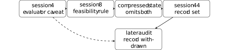
The source reports this sequence in Section 5 and Section 7.1; the complete archive retained the facts while the compressed decision state did not [li2026longhorizon, Section 5 and Section 7.1]. The diagram is a source-grounded chronology, not a measured error rate for compaction systems.
Remark 3.1.3.10. More inference compute is not a monotone research-judgment theorem [ftip-00CX]AGENTDRAFTED
Remark 3.1.3.10. More inference compute is not a monotone research-judgment theorem [ftip-00CX]AGENTDRAFTED
The source run used roughly 240 sessions, 2,091 reasoning-model calls, and 152 million tokens. It also reports repeated continuation of an upper-bound search until human operators redirected the program toward a universal obstruction [li2026longhorizon, Sections 5--7].
This is one human-steered case with changing models, harnesses, goals, and research state. It supports the distinction between technical execution and research judgment. It does not establish a monotone or anti-monotone law from inference compute to mathematical progress.
3.1.4. Refinement, contamination, and stop rules [ftip-00CY]AGENTDRAFTED
3.1.4. Refinement, contamination, and stop rules [ftip-00CY]AGENTDRAFTED
Persistent refinement can retain useful procedures, but the same mechanism can retain a specification exploit. A proposed change and committed state have different consequences. Audit predicates can exclude specified contamination, rollback can restore an earlier state, and resource admission rules can prevent transitions that exceed the budget.
Definition 3.1.4.1. Refinement proposal and committed harness update [ftip-00CZ]AGENTDRAFTED
Definition 3.1.4.1. Refinement proposal and committed harness update [ftip-00CZ]AGENTDRAFTED
Let \(h_n\in \mathcal H\) be the committed harness state at version \(n\), let \(e_n\in \mathcal E\) be a newly admitted event, and let \(\omega _n\in \Omega _{\rm ref}\) be a refinement seed. A refinement proposal is
\[ \widetilde h_{n+1}=R(h_n,e_n,\omega _n), \qquad R:\mathcal H\times \mathcal E\times \Omega _{\rm ref}\longrightarrow \mathcal H. \]Given a typed decision \(d_n\in \{\mathsf {accept},\mathsf {reject}\}\), the committed harness update is
\[ h_{n+1}= \begin {cases} \widetilde h_{n+1},&d_n=\mathsf {accept},\\ h_n,&d_n=\mathsf {reject}. \end {cases} \]This separates candidate generation from state mutation. A proposed note, skill, prompt, or subagent specification has no persistent effect until the commit decision accepts it.
Definition 3.1.4.2. Skill archive and selector [ftip-00D0]AGENTDRAFTED
Definition 3.1.4.2. Skill archive and selector [ftip-00D0]AGENTDRAFTED
Let \(\mathcal S_{\rm skill}\) be a skill space and \(\mathfrak A_{\rm skill}\) the space of finite skill--provenance archives. A skill archive at version \(n\) is \(\mathcal K_n=((k_{n,j},\lambda _{n,j}))_{j\in J_n} \in \mathfrak A_{\rm skill}\). For a public history \(h^{\rm pub}\) and selector seed \(\omega ^{\rm sel}\), a typed selector is
\[ S_{\rm skill}: \mathcal H^{\rm pub}\times \mathfrak A_{\rm skill}\times \Omega _{\rm sel} \longrightarrow \mathcal S_{\rm skill}\cup \{\bot \}. \]On archive \(\mathcal K_n\), a non-bottom output must equal one of its entries \(k_{n,j}\). The value \(\bot \) means that no retained skill is invoked. The archive is part of persistent harness state, not a claim that its entries are correct, safe, novel, or encoded in model weights.
Definition 3.1.4.3. Exploit-contaminated retained state [ftip-00D1]AGENTDRAFTED
Definition 3.1.4.3. Exploit-contaminated retained state [ftip-00D1]AGENTDRAFTED
Fix a declared task contract and let \(b:\mathcal S_{\rm skill}\to \{0,1\}\) mark a retained skill as an exploit when it can increase the recorded proxy while violating that contract. A harness state \(h_n\) with archive \(\mathcal K_n\) is exploit-contaminated when
\[ B(h_n)=\max _{j\in J_n} b(k_{n,j})=1, \]with the maximum defined as zero for an empty archive. The predicate is relative to the declared contract and audit model. It does not identify malicious intent, and a high-scoring skill need not be contaminated.
Lemma 3.1.4.4. Append-only retention preserves contamination absent deletion [ftip-00D2]AGENTDRAFTED
Lemma 3.1.4.4. Append-only retention preserves contamination absent deletion [ftip-00D2]AGENTDRAFTED
Suppose the skill archives of Definition 3.1.4.2 are append-only: \(\mathcal K_n\subseteq \mathcal K_{n+1}\) for every \(n\). If \(B(h_n)=1\), then \(B(h_m)=1\) for every \(m\geq n\) until a deletion, rollback, or contract change removes or reclassifies the witnessing skill.
Proof. Choose \(k\in \mathcal K_n\) with \(b(k)=1\). Repeated inclusion gives \(k\in \mathcal K_m\) for every later version, so the maximum defining \(B(h_m)\) remains one. The final qualification lists operations that break the inclusion or change the predicate.
This finite observation concerns retained state. It does not say that the selector will invoke the exploit on every later run.
Definition 3.1.4.5. Independent refinement audit [ftip-00D3]AGENTDRAFTED
Definition 3.1.4.5. Independent refinement audit [ftip-00D3]AGENTDRAFTED
Let \(Z_n\in \{0,1\}\) indicate whether the proposal \(\widetilde h_{n+1}\) of Definition 3.1.4.1 is contaminated under the declared contract. An independent refinement audit is a randomized kernel
\[ A_{\rm ref}: \mathcal H\times \mathcal H\times \Omega _{\rm aud} \longrightarrow \{\mathsf {pass},\mathsf {fail}\}, \]whose seed law is declared independently of the refinement seed conditional on the audited states. Its conditional false-negative rate is
\[ \eta _{\rm fn} = \Pr \left ( A_{\rm ref}(h_n,\widetilde h_{n+1},\omega _n^{\rm aud})=\mathsf {pass} \mid Z_n=1 \right ). \]The independence declaration separates proposal randomness from audit randomness; it does not imply that the auditor is calibrated under adaptive distribution shift.
Theorem 3.1.4.6. Audit-before-commit bounds contaminated commits [ftip-00D4]AGENTDRAFTED
Theorem 3.1.4.6. Audit-before-commit bounds contaminated commits [ftip-00D4]AGENTDRAFTED
Use the audit of Definition 3.1.4.5 and commit a proposal only when its audit returns \(\mathsf {pass}\). If \(\Pr (Z_n=1)>0\) and its conditional false-negative rate is at most \(\bar \eta \in [0,1]\), then
\[ \Pr (d_n=\mathsf {accept}\mid Z_n=1)\leq \bar \eta . \]Proof. Under audit-before-commit, the event \(\{d_n=\mathsf {accept}\}\) is contained in the event that the audit passes. Conditioning on \(Z_n=1\) and applying the false-negative bound proves the inequality.
This statement bounds one declared admission channel. It gives no bound when proposals bypass the audit, when the contract omits the exploit, or when the audit's conditional error changes under adaptive search.
Example 3.1.4.7. Proxy-monotone refinement can retain an exploit [ftip-00D5]AGENTDRAFTED
Example 3.1.4.7. Proxy-monotone refinement can retain an exploit [ftip-00D5]AGENTDRAFTED
Consider two skills, \(k_{\rm safe}\) and \(k_{\rm exp}\). Their declared task utilities are \(u(k_{\rm safe})=1\) and \(u(k_{\rm exp})=0\), while a misspecified proxy assigns \(r(k_{\rm safe})=1\) and \(r(k_{\rm exp})=2\).
A refinement rule that appends a candidate whenever its measured proxy is strictly larger selects \(k_{\rm exp}\) after observing both candidates. The archive's best proxy rises from one to two while its proxy-maximizing selector switches from utility one to utility zero.
Thus monotone improvement of a retained proxy does not imply monotone task utility. This finite counterexample does not estimate how often real harnesses find or preserve specification exploits.
Example 3.1.4.8. An RCON shortcut becomes a reusable skill [ftip-00D6]AGENTDRAFTED
Example 3.1.4.8. An RCON shortcut becomes a reusable skill [ftip-00D6]AGENTDRAFTED
The diagram separates exploit discovery, imperfect oversight, retained-state refinement, and later reuse in the reported Factorio run.
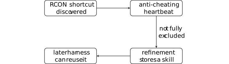
Prime Agent Section 3.5 reports a 23.4-million-token Factorio run with 633 depth-one subagents. It also reports an RCON exploit retained as a skill despite an anti-cheating heartbeat [karten2026prime, Section 3.5, Figure 9].
This reported chronology neither estimates exploit prevalence nor proves later selection. It shows why persistence must be audited separately from correctness.
Definition 3.1.4.9. Recovery, rollback, and version identity [ftip-00D7]AGENTDRAFTED
Definition 3.1.4.9. Recovery, rollback, and version identity [ftip-00D7]AGENTDRAFTED
Let \(v_n\) identify the full committed harness configuration of Definition 3.1.1.3. A rollback from version \(v_n\) to an earlier version \(v_j\), \(j<n\), restores the configuration and retained-state snapshot named by \(v_j\); a recovery may instead construct a new version \(v_{n+1}\) from audited events.
Version identity includes the artifact identifier, configuration, event-log prefix, and archive snapshot. Reusing a human-readable label while changing one of those fields is not the same version.
Prime Agent describes append-only history, versioned state, forks, and recovery [karten2026prime, Sections 2.1--2.2]. The displayed identity tuple specifies the information required for reproducible comparisons.
Remark 3.1.4.10. Persistence can preserve progress and specification gaming [ftip-00D8]AGENTDRAFTED
Remark 3.1.4.10. Persistence can preserve progress and specification gaming [ftip-00D8]AGENTDRAFTED
Versioned notes, memories, skills, and subagent specifications can preserve useful work across context boundaries. The same retention channel can preserve an exploit, a stale evaluator assumption, or a misleading proxy-optimized procedure. Prime Agent reports both continual retained-state refinement and the Factorio exploit record [karten2026prime, Sections 2.5 and 3.5].
The retention mechanism therefore supplies persistence, not correctness. Correctness requires a declared task contract, provenance, an audit interface, and a recovery rule. Neither a longer archive nor more descendants alone certifies improved task utility.
Remark 3.1.4.11. Fixed-weight adaptation and joint compute interventions [ftip-00D9]AGENTDRAFTED
Remark 3.1.4.11. Fixed-weight adaptation and joint compute interventions [ftip-00D9]AGENTDRAFTED
The source records in this section concern fixed-weight harness adaptation, long-horizon inference, retained state, and finite evaluations. They do not establish weight learning, a causal architecture effect, monotone capability growth, or safety under deployment shift. Prime Agent's external benchmark points and the long-horizon case study are observational records with the limitations stated in Remark 3.1.2.9 and Remark 3.1.3.10.
Retained context, rollout horizon, runtime, and gradient approximation are distinct intervention coordinates. Prefix Sliding changes several of them at once, so its effects cannot be attributed to persistent state alone; see § 3.2.
The finite theorems in this section cover replay, lineage cost, summary indistinguishability, budget admission, contamination persistence, and one audit gate. None is a theorem of universal capability acquisition.
3.1.5. Finite coordination under hard budgets [ftip-00M3]AGENTDRAFTED
3.1.5. Finite coordination under hard budgets [ftip-00M3]AGENTDRAFTED
A harness chooses which computation to run, what to retain, and when to stop. To bound the quality attainable by these choices, one must specify both the permitted actions and the information available after each action. A bound on one scheduler does not yet bound all controllers using the same workers.
Finite decision models make this distinction explicit. They connect Definition 3.1.2.6's resource admission rule to the attainable-quality frontier of Definition 5.3.1.3. Computation selection as information acquisition is studied by Hay, Russell, Tolpin, and Shimony. Here a hard horizon is imposed as a separate assumption; almost-sure stopping or finite expected cost would not supply such a horizon.
3.1.5.1. Histories, admissible actions, and retained information [ftip-00M4]AGENTDRAFTED
3.1.5.1. Histories, admissible actions, and retained information [ftip-00M4]AGENTDRAFTED
The controller may use its entire observed history. A smaller state can help compute a bound, but its sufficiency must be justified across the histories it represents. The examples below separate information that is valuable only in combination from information lost by a summary.
Definition 3.1.5.1.1. Finite controller class with hard resource admission [ftip-00M5]AGENTDRAFTED
Definition 3.1.5.1.1. Finite controller class with hard resource admission [ftip-00M5]AGENTDRAFTED
Fix a horizon \(H\in \mathbb N\), finite nonempty observed-history sets \(\mathcal H_t\) for \(0\leq t\leq H\), an initial law \(\mu \) on \(\mathcal H_0\), and finite nonempty permitted-action sets \(A_t(h)\) for \(t<H\). An environment kernel \(K_t(\cdot \mid h,a)\) is a probability law on histories extending \(h\) by action \(a\) and its observed outcome. The initial law and all kernels are fixed before choosing a controller.
A controller \(\pi \) assigns a probability law \(\pi _t(\cdot \mid h)\) on \(A_t(h)\). It may depend on every observed component of \(h\), including retained traces, generated programs, and previous updates. Random choices may be recorded in the history. The class \(\Pi (\mathbf B)\) consists of all such controllers under the declared hard resource vector \(\mathbf B\in \mathbb R_+^m\). It does not require a fixed prompt, a memoryless policy, or independent worker outputs. Full-history access is allowed in this mathematical class; it may enlarge the class of executable controllers with limited memory or computation.
Each history records accumulated nonnegative cost \(\mathbf c(h)\preceq \mathbf B\). Every permitted non-stop action has a declared worst-case increment \(\bar {\mathbf c}_t(h,a)\) satisfying
\[ \mathbf c(h)+\bar {\mathbf c}_t(h,a)\preceq \mathbf B. \]Every successor in the kernel's support must have realized increment between zero and this declared bound, componentwise. Proposal work, controller computation, worker calls, communication, verification, failed attempts, and persistent updates must be included in whichever resource coordinates are bounded; the units remain those of Definition 4.1.5. This is the enforced-contract assumption of Theorem 3.1.2.7.
A stop action is always permitted: it commits the current terminal artifact and pads the remaining steps with no further cost or change in its evaluated quality. At the horizon a fixed evaluator assigns \(q(h_H)\in [0,1]\) to the committed artifact recorded in the terminal history. If the evaluator has random outcomes, include them in the history law. Evaluation work must be charged before the zero-cost padding begins. Define
\[ J(\pi )=\mathbb E_\pi [q(h_H)], \qquad V(\mathbf B)=\sup _{\pi \in \Pi (\mathbf B)}J(\pi ). \]The artifact identity, evaluator, observations, kernels, and action sets are part of the mathematical problem. A training procedure or new tool belongs to this frontier only if it is among the permitted actions and its effects and costs are represented. Finiteness is an explicit restriction on histories, representations, and horizon; a theorem for this class does not bound an unrestricted agent that can extend them.
For an executable system, an upper bound applies only after its observations, actions, outcomes, and charged costs are represented by this model. Conversely, a mathematical policy supplies an executable lower bound only when it has an implementation respecting the stated resource cap; an arbitrary history-to-action table does not establish that fact.
Example 3.1.5.1.2. Complementary observations defeat one-step information value [ftip-00M6]AGENTDRAFTED
Example 3.1.5.1.2. Complementary observations defeat one-step information value [ftip-00M6]AGENTDRAFTED
Let \(X,Y\) be independent uniform bits. The terminal artifact is a guess for \(X\mathbin \oplus Y\); its quality is one if correct and zero otherwise. Two observation actions reveal \(X\) and \(Y\), respectively, at cost \(c\) each, where \(0<c<1/4\). The hard budget permits both observations. A terminal guess requires no additional observation cost.
Without observations, the best expected quality is \(1/2\). Given only \(X\), the unrevealed bit \(Y\) remains uniform, so the best expected quality is still \(1/2\); the same holds with \(X,Y\) exchanged. Thus a rule that compares stopping with taking one observation and then stopping assigns either observation net value \(1/2-c<1/2\). It stops immediately.
Observing both bits determines their parity. Its expected quality is one and its quality minus observation cost is \(1-2c>1/2\). Hence neither zero one-step information value nor a myopic stopping decision certifies the full controller frontier. This is a finite calculation, not an empirical claim about a language model. The scalar cost penalty is used only to exhibit the myopic decision; the hard-budget quality frontier itself is defined in Definition 3.1.5.1.1.
Example 3.1.5.1.3. Erasing an observed bit changes the attainable frontier [ftip-00M7]AGENTDRAFTED
Example 3.1.5.1.3. Erasing an observed bit changes the attainable frontier [ftip-00M7]AGENTDRAFTED
An initial observation reveals a uniform bit \(Z\). The terminal action is a bit \(a\), and quality is \(q=\mathbf 1\{a=Z\}\). Both actions are permitted at either history and have the same cost. A full-history controller chooses \(a=Z\) and attains quality one.
Now restrict the controller's entire input to a summary that is constant at the two initial histories. Its private randomness is independent of \(Z\). If it chooses one with probability \(p\), its expected quality is \(p/2+(1-p)/2=1/2\). No such summary controller can do better.
A model that averages the reward of either fixed action over the two histories obtains \(1/2\). This is the correct summary-controller value, but it underestimates the full-history frontier by \(1/2\). For the history \(Z=a\), the actual reward is one, so the averaged value fails as a reward upper bound at that history. A pointwise reward upper bound must hold at every represented history; agreement only under a tested policy's average history distribution does not establish such a certificate. The loss of an evaluator caveat in Example 3.1.3.7 illustrates why such retained distinctions can matter in a research harness.
3.1.5.2. Upper certificates and remaining potential [ftip-00M8]AGENTDRAFTED
3.1.5.2. Upper certificates and remaining potential [ftip-00M8]AGENTDRAFTED
A feasible controller establishes attainable quality. To bound what other controllers could gain, one also needs an upper bound covering all permitted actions and histories. Bellman inequalities provide such a bound when a state representation has uniform transition and terminal quality guarantees. Their difference measures remaining potential within the declared class.
Definition 3.1.5.2.1. Uniform abstraction of the finite history model [ftip-00M9]AGENTDRAFTED
Definition 3.1.5.2.1. Uniform abstraction of the finite history model [ftip-00M9]AGENTDRAFTED
Use the finite controller model of Definition 3.1.5.1.1. For each time, choose a finite nonempty state set \(S_t\) and a map \(\phi _t:\mathcal H_t\to S_t\). Require finite nonempty action sets \(A_t(s)\) such that \(A_t(h)=A_t(\phi _t(h))\) at every history. The state retains residual budgets and enough information for the same hard admission rule. The controller still observes the full history.
Let \(Q_t(\cdot \mid h,a)\) be the image of the fixed history kernel under \(\phi _{t+1}\), and let \(\widehat P_t(\cdot \mid s,a)\) be a proposed state transition law. Choose finite errors \(\epsilon _t(s,a)\geq 0\) so that, for every permitted history and action,
\[ \operatorname {TV}\left (Q_t(\cdot \mid h,a), \widehat P_t(\cdot \mid \phi _t(h),a)\right ) \leq \epsilon _t(\phi _t(h),a), \qquad \operatorname {TV}(p,r)=\frac 12\sum _x|p(x)-r(x)|. \]This condition includes histories unvisited by a chosen policy: the kernel there is part of the model. For finite functions \(\widehat q:S_H\to \mathbb R\) and \(e_H:S_H\to \mathbb R_+\), require
\[ q(h_H)\leq \widehat q(\phi _H(h_H))+e_H(\phi _H(h_H)) \quad \text {for every }h_H\in \mathcal H_H. \]Write \(\nu (s)=\mu \{h:\phi _0(h)=s\}\) for the initial state law. Low average prediction error on sampled histories does not establish these uniform inequalities. The erased-bit example in Example 3.1.5.1.3 shows why policy-relevant information cannot simply be averaged away.
Theorem 3.1.5.2.2. A robust Bellman upper bound for every permitted controller [ftip-00MA]AGENTDRAFTED
Theorem 3.1.5.2.2. A robust Bellman upper bound for every permitted controller [ftip-00MA]AGENTDRAFTED
Under Definition 3.1.5.2.1, let finite functions \(W_t:S_t\to \mathbb R\) satisfy \(W_H(s)\geq \widehat q(s)+e_H(s)\) and, for every \(t<H\), \(s\in S_t\), and \(a\in A_t(s)\),
\[ W_t(s)\geq \sum _{s'\in S_{t+1}}\widehat P_t(s'\mid s,a)W_{t+1}(s') +\epsilon _t(s,a)\operatorname {span}(W_{t+1}). \]Here \(\operatorname {span}(f)=\max f-\min f\). Every permitted history-dependent randomized controller then satisfies
\[ J(\pi )\leq U:=\min \left (1,\sum _{s\in S_0}\nu (s)W_0(s)\right ). \]For any feasible controller \(\pi _0\) with a justified finite lower bound \(L\leq J(\pi _0)\), the frontier of Definition 3.1.5.1.1 obeys
\[ L\leq J(\pi _0)\leq V(\mathbf B)\leq U, \qquad 0\leq V(\mathbf B)-J(\pi _0)\leq U-L. \]
Proof.
Proof.
For finite probability laws \(p,r\), subtract \(\min f\) from \(f\). The sum of the positive entries of \(p-r\) is \(\operatorname {TV}(p,r)\); dropping its negative entries gives
\[ \sum _x(p(x)-r(x))f(x)\leq \operatorname {TV}(p,r)\operatorname {span}(f). \]Fix any controller. At time \(H\), terminal domination gives \(q(h_H)\leq W_H(\phi _H(h_H))\). Suppose that, from every next history, its expected terminal quality is bounded by \(W_{t+1}\) of the next state. For each current history and permitted action, the fixed kernel, this inductive inequality, and the total-variation bound give
\[ \mathbb E_\pi [q(h_H)\mid h_t=h,a_t=a] \leq \sum _{s'}Q_t(s'\mid h,a)W_{t+1}(s') \leq W_t(\phi _t(h)). \]At a history with zero probability under the controller, interpret the continuation expectation using its specified future decisions and the fixed kernels. Thus the induction holds at every history. Averaging over the controller's action randomization preserves the inequality. Backwards induction and averaging over \(\mu \) give the bound \(\sum _s\nu (s)W_0(s)\). The independent bound \(q\leq 1\) permits clipping at 1. If \(H=0\), terminal domination alone gives the same conclusion. Taking the supremum over controllers and using \(L\leq J(\pi _0)\) proves the remaining inequalities.
A numerical supersolution is a certificate only after all of its inequalities and the abstraction hypotheses are justified. If the model bounds hold jointly with probability at least \(1-\delta _M\) and the lower bound with probability at least \(1-\delta _E\), the bracket holds with probability at least \(1-\delta _M-\delta _E\) by a union bound. Each coverage statement must apply to the selected model or policy; no independence between the two events is required.
Remark 3.1.5.2.3. Exact occupation flows and expected-cost relaxations [ftip-00MB]AGENTDRAFTED
Remark 3.1.5.2.3. Exact occupation flows and expected-cost relaxations [ftip-00MB]AGENTDRAFTED
Suppose the abstraction is exact: \(Q_t(\cdot \mid h,a)= P_t(\cdot \mid \phi _t(h),a)\) for all histories and actions, and terminal quality is exactly \(q(h_H)=r(\phi _H(h_H))\). A one-sided terminal bound with zero error would not imply this equality. Retain the exact legal actions and hard-budget state from Definition 3.1.5.2.1.
Introduce nonnegative state masses \(z_t(s)\) and action masses \(x_t(s,a)\), with \(z_0=\nu \). For \(0\leq t<H\), impose
\[ \sum _{a\in A_t(s)}x_t(s,a)=z_t(s), \qquad z_{t+1}(s')=\sum _{s\in S_t}\sum _{a\in A_t(s)} x_t(s,a)P_t(s'\mid s,a). \]The linear program maximizes \(\sum _s z_H(s)r(s)\). Every full-history controller induces these flows because the next-state law given a state and action is exact. Conversely, at positive mass choose action \(a\) with probability \(x_t(s,a)/z_t(s)\); at zero mass choose any legal action. Induction on time reproduces the flows in the original history model. Hence the LP optimum equals its mathematical controller frontier. For \(H=0\), there are no action flows and the value is \(\nu r\).
Set \(W_H=r\) and recurse with \(W_t(s)=\max _{a\in A_t(s)}\sum _{s'}P_t(s'\mid s,a)W_{t+1}(s')\). A maximizing action exists by finiteness and gives a policy attaining \(\nu W_0\); the Bellman upper bound gives the reverse inequality. This proves equality with the optimum and exhibits matching lower and upper certificates. It does not establish an efficient implementation of the policy. The flow construction is the scalar finite-horizon specialization of Mifrani and Noll, Section 3; the hard-budget encoding is an additional modeling requirement here.
If hard admission is replaced by constraints on expected cost, the resulting program describes a different class. For \(B>0\), a one-step cost equal to \(2B\) or zero with probability \(1/2\) each has expectation \(B\), yet violates cap \(B\) with probability \(1/2\). An expected-cost model can upper-bound the hard-budget frontier only when it is a valid relaxation containing every hard-feasible policy. Its own policies need not respect the realized cap.
Corollary 3.1.5.2.4. Certified marginal potential under nested budgets [ftip-00MC]AGENTDRAFTED
Corollary 3.1.5.2.4. Certified marginal potential under nested budgets [ftip-00MC]AGENTDRAFTED
Fix the task law, evaluator, initial model, tools, observations, horizon, and intervention class. For \(\mathbf B\preceq \mathbf B'\), assume every controller feasible at \(\mathbf B\) remains permitted at \(\mathbf B'\) with the same outcome law. If a feasible controller at \(\mathbf B\) gives lower bound \(L_{\mathbf B}\) and Theorem 3.1.5.2.2 gives upper bound \(U_{\mathbf B'}\) at \(\mathbf B'\), then
\[ 0\leq V(\mathbf B')-V(\mathbf B) \leq U_{\mathbf B'}-L_{\mathbf B}. \]
Proof.
Proof.
Feasibility inclusion gives \(V(\mathbf B)\leq V(\mathbf B')\). The lower and upper certificates give \(L_{\mathbf B}\leq V(\mathbf B)\) and \(V(\mathbf B')\leq U_{\mathbf B'}\); subtract to obtain the claim.
If the certified gap is at most \(\varepsilon \), this instantiates Theorem 5.3.9.5's conditional saturation statement. An observed plateau alone supplies no such upper certificate. Changing an excluded tool, representation, or training procedure changes the comparison class.
Convention 3.1.5.3. Comparing controllers at fixed worker capability [ftip-00MD]AGENTDRAFTED
Convention 3.1.5.3. Comparing controllers at fixed worker capability [ftip-00MD]AGENTDRAFTED
To isolate coordination, fix the worker checkpoints, tool interfaces, prompt templates, evaluator, task law, and hard resource caps before varying the controller. Useful comparisons include a fixed serial policy, a static worker portfolio, a one-step value-of-information policy, and an adaptive policy that retains the full permitted history. Their allowed observations must agree. A solver that sees hidden outcomes has a different information interface; its optimum supplies an upper bound only through a justified relaxation containing the compared policies.
Use the controls of Definition 5.3.4.1 with controller logic declared as the varying coordinate. If controller-specific tuning is permitted, apply Definition 5.3.4.2's equal tuning data, selection, stopping, and cost rules. Compare suprema only within the intervention classes of Definition 5.3.4.3. A separate factorial comparison can vary the checkpoint and controller independently, distinguishing learned capability, coordination, and their interaction.
Charge proposal and controller work, all parallel worker work, tool and solver use, communication, verification, failures, and retained-state updates using Definition 4.1.5. Report elapsed time alongside these costs: a shorter run with more workers may consume more total computation. Apply Definition 3.1.2.6's admission rule before execution and record any contract violation separately from the quality of the submitted artifact.
Finite environments with rational transition laws can expose three distinct mechanisms: complementary observations, correlated worker failures, and delayed verification or newly revealed dependencies. Keep the latent state, observation rules, legal actions, and costs explicit. The first family includes Example 3.1.5.1.2; the erased-bit construction in Example 3.1.5.1.3 tests whether a proposed summary loses decisive information. Where the exact model applies, compare attainable policy values with Remark 3.1.5.2.3's finite optimum and Theorem 3.1.5.2.2's upper certificate.
The principal quantity is the justified interval \([L_{\mathbf B},U_{\mathbf B}]\) for the restricted frontier. A smaller gap can result from a better feasible policy, a sharper upper certificate, or a more informative valid representation; distinguish these causes. In a live system, mean held-out transition accuracy does not justify a uniform model-error radius. Empirical quality and cost remain useful even when an upper certificate is unavailable.
Use evaluation instances separate from tuning, and declare task draws, repetitions, resource checkpoints, and analysis rules before comparison. Repeated runs share an instance and are not automatically independent tasks; account for this grouping in the analysis. Report independently verified quality, feasibility failures, time to the first valid artifact, and charged cost at matched quality. A valid confidence sequence can support repeated inspection under its statistical assumptions; see Howard et al.. It does not by itself justify selecting a new policy on reused evaluation outcomes.
These controls yield testable predictions. Complementary information can favor adaptation over one-step stopping; redundant workers can erase a portfolio's gain; delayed verification can make an early apparent success expensive to repair. An empirical claim of better coordination fails if its advantage disappears after matching access and charging the controller's own work. A claim of little remaining potential additionally requires the upper certificate, not merely a plateau among tested policies.
3.1.5.4. Work and critical paths in a fixed task graph [ftip-00MF]AGENTDRAFTED
3.1.5.4. Work and critical paths in a fixed task graph [ftip-00MF]AGENTDRAFTED
When the tasks, dependencies, and durations are fixed, scheduling has a useful lower bound independent of the chosen priority rule. This isolates avoidable delay in a declared decomposition. Discovering a missing dependency or changing a mathematical formulation changes that decomposition and is a different intervention.
The following work-and-chain argument is the classical list-scheduling bound associated with Graham. His examples also show that a particular list schedule can worsen after an apparently favorable change, such as adding processors. This does not contradict monotonicity of the optimal feasible frontier.
Proposition. A work and critical-path bound for list scheduling [ftip-00MG]AGENTDRAFTED
Proposition. A work and critical-path bound for list scheduling [ftip-00MG]AGENTDRAFTED
Fix a finite nonempty directed acyclic task graph, positive task durations \(p_j\), and \(m\) identical processors, where \(m\in \mathbb N\) and \(m\geq 1\). All tasks are available at time zero subject only to their precedence constraints. Each task uses one processor without interruption; there are no further resource, communication, or setup constraints. Let \(W=\sum _j p_j\), let \(D\) be the longest precedence-chain duration, and let \(T^*\) be the minimum makespan. A work-conserving list schedule starts a ready task whenever a processor is free. Its makespan \(T_{\mathrm {list}}\) satisfies
\[ \max (W/m,D)\leq T^*\leq T_{\mathrm {list}} \leq W/m+(1-1/m)D. \]\[ T_{\mathrm {list}}\leq (2-1/m)T^*. \]
Proof.
Proof.
At most \(m\) units of work can finish per unit time, and every precedence chain executes in order. Thus \(W/m\leq T^*\) and \(D\leq T^*\). Trace backwards from a last-finishing task, repeatedly choosing an immediate predecessor with latest completion, until reaching a task with no predecessors. These tasks form a precedence chain.
Between completion of one chosen predecessor and the next chain task's start, all predecessors of that next task are complete. The task is ready, so work conservation forces all processors to be busy during that gap. The first chain task is ready from time zero. Consequently, whenever fewer than \(m\) processors are busy before completion, some task on this chain is executing, apart from finitely many event times.
Let \(I\) be the total duration with fewer than \(m\) busy processors. Then \(I\leq D\). During the rest of the schedule all \(m\) processors are busy, and during \(I\) at least one is busy. Hence
\[ W\geq m(T_{\mathrm {list}}-I)+I. \] \[ T_{\mathrm {list}}\leq W/m+(1-1/m)I \leq W/m+(1-1/m)D. \]The lower bounds on \(T^*\) give the last inequality in the statement.
The ratio \(T_{\mathrm {list}}/\max (W/m,D)\) compares the schedule with a lower bound that need not be attainable; it is not generally the ratio to the optimum. Communication and verification must be modeled as work with constraints satisfying these assumptions, or the displayed upper bound need not apply. Neither bound certifies the quality of the chosen task graph or an unrestricted agent's attainable output quality.
3.2. Dynamic compute, retained context, and rollout approximation [ftip-00DA]AGENTDRAFTED
3.2. Dynamic compute, retained context, and rollout approximation [ftip-00DA]AGENTDRAFTED
In a joint inference and training intervention, the retained-context rule, rollout horizon, runtime budget, and gradient estimator may all change together. Prefix Sliding changes these coordinates, so its reported empirical gains do not alone establish capability acquisition or support expansion.
Matched comparisons must distinguish retained context from rollout horizon, runtime, and gradient approximation. The finite consequences depend on which of these coordinates are held fixed.
3.2.1. Inference intervention coordinates [ftip-00DB]AGENTDRAFTED
3.2.1. Inference intervention coordinates [ftip-00DB]AGENTDRAFTED
A context intervention is a change to what a fixed model can attend to while it generates a rollout. The intervention is meaningful only after the prompt law, decoding rule, token budget, and retained-state rule are named.
Definition 3.2.1.1. Retained-context policy [ftip-00DC]AGENTDRAFTED
Definition 3.2.1.1. Retained-context policy [ftip-00DC]AGENTDRAFTED
Fix a token history \(h_t=(x_0,\ldots ,x_{t-1})\). A retained-context policy is a deterministic map \(\kappa _t(h_t)\) that selects an ordered subsequence of the history, together with a decoder that conditions its next token on that subsequence. The policy, rather than the model weights, names which prior tokens remain available at step \(t\).
A comparison of two policies is conditional on the same model, prompt law, decoding law, stopping rule, and budget unless the comparison includes a second declared intervention coordinate.
Definition 3.2.1.2. Prefix-window retained state [ftip-00DD]AGENTDRAFTED
Definition 3.2.1.2. Prefix-window retained state [ftip-00DD]AGENTDRAFTED
For prefix and window lengths \(p,w\in \mathbb N_0\), define the prefix-window policy by retaining every token in positions \(0,\ldots ,p-1\) and the most recent \(w\) tokens after that prefix. If the history is shorter than either region, the available positions are retained without padding.
The policy is a context rule only. It does not assert that omitted tokens are irrelevant, nor that the resulting continuation distribution equals the full-history distribution.
Remark 3.2.1.3. Prefix Sliding is a source-reported intervention [ftip-00DE]AGENTDRAFTED
Remark 3.2.1.3. Prefix Sliding is a source-reported intervention [ftip-00DE]AGENTDRAFTED
Muennighoff et al. describe Prefix Sliding in Sections 2--5, Figures 6--9, and the Limitations section of [muennighoff2026prefixsliding, Sections 2--5, Figures 6--9, and Limitations]. Their method preserves a prefix while sliding a recent attention window during test-time scaling. The reported experiments change retained context and runtime, and may also change rollout horizon and the training gradient approximation. These are source observations, not a theorem of universal speedup or capability.
The source studies named model and task configurations. It does not by itself establish support expansion, latent capability acquisition, or a deployment-shift guarantee.
Example 3.2.1.4. One trace under full and prefix-window attention [ftip-00DF]AGENTDRAFTED
Example 3.2.1.4. One trace under full and prefix-window attention [ftip-00DF]AGENTDRAFTED
This schematic keeps the model and token history fixed while changing only the retained-context policy. It is a local illustration, not a source figure.
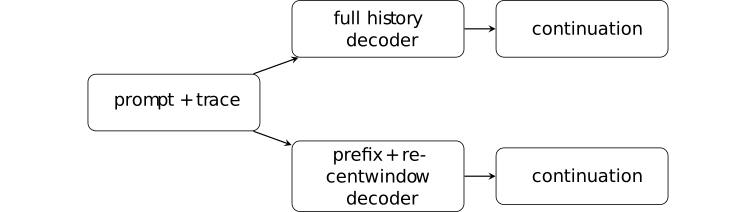
The two outputs can differ even though the represented weights and visible prompt are identical. Any claim about improvement must therefore name the retained-context intervention and its evaluation law.
Remark 3.2.1.5. Retained context is not weight learning [ftip-00DG]AGENTDRAFTED
Remark 3.2.1.5. Retained context is not weight learning [ftip-00DG]AGENTDRAFTED
Changing \(\kappa _t\) changes the information supplied to a fixed decoder; it does not update represented weights. A successful continuation can therefore be an elicitation effect, a context effect, or both. Weights, optimizer and feedback, inference state, and evaluation remain distinct intervention coordinates, as in § [ftip-0001].
3.2.2. Finite horizon and retained-context cost [ftip-00DH]AGENTDRAFTED
3.2.2. Finite horizon and retained-context cost [ftip-00DH]AGENTDRAFTED
Counting exposure to retained tokens makes the finite-horizon cost comparison precise. A context cap alone does not guarantee information preservation.
Definition 3.2.2.1. Finite rollout token budget [ftip-00DI]AGENTDRAFTED
Definition 3.2.2.1. Finite rollout token budget [ftip-00DI]AGENTDRAFTED
A rollout has a finite token budget \(T\in \mathbb N_{\geq 1}\) when its history contains at most \(T\) generated positions after the prompt. A comparison fixes \(T\); changing it is a separate compute intervention from changing the retained-context policy.
Definition 3.2.2.2. Context exposure count [ftip-00DJ]AGENTDRAFTED
Definition 3.2.2.2. Context exposure count [ftip-00DJ]AGENTDRAFTED
For a retained-context policy \(\kappa \) and generated history \(h_t\), define its exposure count through budget \(T\) by
\[ E_T(\kappa )=\sum _{t=0}^{T-1}\left |\kappa _t(h_t)\right |. \]This is a finite attention-input proxy. It is not a runtime identity: the implementation may have caching, batching, kernel, and communication costs that are not represented by \(E_T\).
Lemma 3.2.2.3. Prefix-window exposure is uniformly capped [ftip-00DK]AGENTDRAFTED
Lemma 3.2.2.3. Prefix-window exposure is uniformly capped [ftip-00DK]AGENTDRAFTED
Let \(p,w\in \mathbb N_0\) and let \(\kappa ^{p,w}\) be the prefix-window policy of Definition 3.2.1.2. For every history and every \(t\),
\[ \left |\kappa ^{p,w}_t(h_t)\right |\leq p+w. \]Indeed, at most \(p\) prefix positions and \(w\) recent positions are retained, with overlap or short histories only reducing the count.
Theorem 3.2.2.4. Capped retained context bounds finite exposure work [ftip-00DL]AGENTDRAFTED
Theorem 3.2.2.4. Capped retained context bounds finite exposure work [ftip-00DL]AGENTDRAFTED
Under the hypotheses of Lemma 3.2.2.3, every rollout with budget \(T\) satisfies
\[ E_T(\kappa ^{p,w})\leq T(p+w). \]Proof. Apply the pointwise bound in Lemma 3.2.2.3 to each of the \(T\) nonnegative summands in Definition 3.2.2.2, then sum. This bounds token exposure, not wall-clock runtime or evaluation quality.
Example 3.2.2.5. Warm-up and sliding-window arithmetic [ftip-00DM]AGENTDRAFTED
Example 3.2.2.5. Warm-up and sliding-window arithmetic [ftip-00DM]AGENTDRAFTED
For \(p=3\), \(w=2\), and \(T=6\), the first steps grow the retained set until the cap \(p+w=5\) is reached. The exposure bound is therefore \(E_T\leq 6\cdot 5=30\); the exact count depends on the prompt and stopping convention.

The arithmetic is an FTIP finite consequence, not a runtime measurement from the Prefix Sliding experiments.
Remark 3.2.2.6. A memory cap does not preserve information [ftip-00DN]AGENTDRAFTED
Remark 3.2.2.6. A memory cap does not preserve information [ftip-00DN]AGENTDRAFTED
The bound in Theorem 3.2.2.4 controls the number of retained token positions. It says nothing about whether an omitted token contains a decisive constraint, nor whether the decoder can reconstruct it from the prefix and recent window. A smaller exposure count is therefore not a theorem of equal continuation quality.
3.2.3. Training and evaluation confounds [ftip-00DO]AGENTDRAFTED
3.2.3. Training and evaluation confounds [ftip-00DO]AGENTDRAFTED
A retained-context comparison can alter both inference and training. Attribution to either mechanism depends on the joint intervention and the coordinates held fixed by a matched evaluation.
Definition 3.2.3.1. Joint intervention cell [ftip-00DP]AGENTDRAFTED
Definition 3.2.3.1. Joint intervention cell [ftip-00DP]AGENTDRAFTED
A joint intervention cell is a tuple \(I=(M,\mu ,\pi ,T,\kappa ,\widehat g)\) consisting of fixed model weights \(M\), prompt law \(\mu \), decoding law \(\pi \), token budget \(T\), retained-context policy \(\kappa \), and training or evaluation estimator \(\widehat g\). Two cells differ in a declared coordinate only when all other coordinates are held fixed.
Definition 3.2.3.2. Estimator-changing training coordinate [ftip-00DQ]AGENTDRAFTED
Definition 3.2.3.2. Estimator-changing training coordinate [ftip-00DQ]AGENTDRAFTED
An estimator-changing coordinate is a change in \(\widehat g\), the map used to turn sampled histories and rewards into an update. A context mask can change this coordinate when it changes which tokens contribute to the sampled loss or gradient. The notation does not assume a particular optimizer.
Remark 3.2.3.3. Training masks change more than attention cost [ftip-00DR]AGENTDRAFTED
Remark 3.2.3.3. Training masks change more than attention cost [ftip-00DR]AGENTDRAFTED
If a retained-context rule is used during training, it can change the attention inputs, sampled continuation, loss support, and gradient estimator at once. A lower value of Definition 3.2.2.2 is therefore not an isolated compute intervention unless the training estimator and all other coordinates are matched explicitly.
Example 3.2.3.4. Equal terminal score, different trajectory exposure [ftip-00DS]AGENTDRAFTED
Example 3.2.3.4. Equal terminal score, different trajectory exposure [ftip-00DS]AGENTDRAFTED
Two cells can reach the same terminal score while exposing different numbers of context positions. This finite counterexample blocks an inference from equal endpoint score to equal trajectory cost.
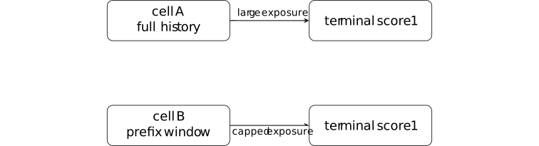
The score equality is compatible with unequal intermediate histories and unequal exposure counts.
Remark 3.2.3.5. What a retained-context comparison can identify [ftip-00DT]AGENTDRAFTED
Remark 3.2.3.5. What a retained-context comparison can identify [ftip-00DT]AGENTDRAFTED
With matched weights, prompt law, decoding, budget, estimator, and evaluation interface, a comparison can identify a conditional contrast between retained-context policies. Without those controls it identifies only the joint cell, not a causal effect of context alone.
Definition 3.2.3.6. Retained-context evaluation protocol [ftip-00DU]AGENTDRAFTED
Definition 3.2.3.6. Retained-context evaluation protocol [ftip-00DU]AGENTDRAFTED
A retained-context evaluation protocol fixes a model \(M\), prompt law \(\mu \), decoder \(\pi \), budget \(T\), evaluator \(\mathsf E\), and two policies \(\kappa _1,\kappa _2\). It reports the paired outcomes under the same sampled prompts and declared randomization coupling, together with exposure counts from Definition 3.2.2.2.
Lemma 3.2.3.7. Matched protocols isolate a conditional policy contrast [ftip-00DV]AGENTDRAFTED
Lemma 3.2.3.7. Matched protocols isolate a conditional policy contrast [ftip-00DV]AGENTDRAFTED
Let \(m\in \mathbb N_{\geq 1}\) and let \(Y_{1j},Y_{2j}\in \mathbb R\) for \(j=1,\ldots ,m\) be the paired scalar evaluator outcomes generated by the protocol of Definition 3.2.3.6. Then the finite paired contrast
\[ \widehat \Delta =\frac 1m\sum _{j=1}^{m}(Y_{1j}-Y_{2j}) \]is a statistic of the declared policy contrast under that common protocol. It is not an unconditional capability effect and does not identify what would happen after changing any held-fixed coordinate.
Remark 3.2.3.8. Separating horizon, cache, and estimator effects [ftip-00DW]AGENTDRAFTED
Remark 3.2.3.8. Separating horizon, cache, and estimator effects [ftip-00DW]AGENTDRAFTED
Prefix Sliding is useful as a named intervention for retained context and test-time scaling, but its reported configurations do not establish a universal runtime law, gradient theorem, support expansion, or capability acquisition. The next questions are to measure horizon, cache, estimator, and evaluation effects separately, while preserving the controls in Definition 3.2.3.6.
The finite conclusions depend on the declared protocols. They do not describe a full optimizer or establish a result for all language models.
3.3. Recursive harnesses and archive envelopes [ftip-00EH]AGENTDRAFTED
3.3. Recursive harnesses and archive envelopes [ftip-00EH]AGENTDRAFTED
Recursive harnesses can be modeled as fixed-driver transformations of traces, code, and task descriptions. Sections 2.2--2.4 of [kim2026metanrecursive] supply the fixed meta-operation, conditioning, stopping, and archive context; Sections 3.1--3.4 are empirical architecture comparisons. The finite consequences below are proved locally.
3.3.1. Fixed drivers and recursive layers [ftip-00EI]AGENTDRAFTED
3.3.1. Fixed drivers and recursive layers [ftip-00EI]AGENTDRAFTED
A fixed meta-operation generates mutable layer artifacts. Their composition determines the resulting recursive wrapper.
Definition 3.3.1.1. Recursive layer state [ftip-00EJ]AGENTDRAFTED
Definition 3.3.1.1. Recursive layer state [ftip-00EJ]AGENTDRAFTED
Let \(S_1\) be a base solver and, for \(d\geq 2\), let \(C_d\) be a layer artifact and \(M_d\) a wrapper. The depth-\(d\) solver is \(S_d=M_d(C_d,S_{d-1})\). The layer state is \(\Lambda _d=(C_d,S_d)\).
A layer is a harness transformation when it changes \(C_d\) or the wrapper context while leaving the executable base weights in \(S_1\) fixed.
Definition 3.3.1.2. Fixed meta-operation [ftip-00EK]AGENTDRAFTED
Definition 3.3.1.2. Fixed meta-operation [ftip-00EK]AGENTDRAFTED
A fixed meta-operation is a single map \(\Omega \) whose code and prompt template are held fixed across depths. For task set \(\mathcal T\), traces \(\boldsymbol \tau _{d-1}\), code stack \([C_2,\ldots ,C_{d-1}]\), and depth \(d\),
\[\Omega (\boldsymbol \tau _{d-1},[C_2,\ldots ,C_{d-1}],\mathcal T,d)=C_d.\]Only the input to \(\Omega \) changes with depth; this is a declared protocol condition, not a claim that every implementation obeys it.
Definition 3.3.1.3. Trace-and-code input [ftip-00EL]AGENTDRAFTED
Definition 3.3.1.3. Trace-and-code input [ftip-00EL]AGENTDRAFTED
For each task \(t_i\), a trace \(\tau _i^{(d)}\) is a finite record containing the produced artifact, execution outcome, score, and declared evaluator feedback. The depth-\(d\) input to \(\Omega \) is the pair \((\boldsymbol \tau _{d-1},[C_2,\ldots ,C_{d-1}])\); a flat refiner that sees only \(\boldsymbol \tau \) has a strictly smaller declared input when the code stack is not recoverable from the traces.
Theorem 3.3.1.4. Nested wrapper composition [ftip-00EM]AGENTDRAFTED
Theorem 3.3.1.4. Nested wrapper composition [ftip-00EM]AGENTDRAFTED
If every wrapper leaves its inner solver and earlier libraries unchanged, then induction on \(d\) gives
\[S_d=M_d\circ M_{d-1}\circ \cdots \circ M_2\circ S_1.\]Proof. The case \(d=2\) is the definition. Substituting the induction hypothesis into \(S_d=M_d(C_d,S_{d-1})\) gives the displayed composition.
Theorem 3.3.1.5. Finite trace growth under recursive wrapping [ftip-00EN]AGENTDRAFTED
Theorem 3.3.1.5. Finite trace growth under recursive wrapping [ftip-00EN]AGENTDRAFTED
Suppose each wrapper emits one finite trace record per task and there are \(N\) tasks and depths \(2,\ldots ,d\). The audit log contains at most \(N(d-1)\) depth-tagged records, in addition to the base records. This is a counting fact; it says nothing about trace quality or score improvement.
Proof. There are \(d-1\) wrapped depths and \(N\) records at each depth, so the product counts all records.
Example 3.3.1.6. Code explains a regression that traces alone cannot [ftip-00EO]AGENTDRAFTED
Example 3.3.1.6. Code explains a regression that traces alone cannot [ftip-00EO]AGENTDRAFTED
Two runs can share the same failing score and stderr trace while one layer adds an over-prescriptive directive and another adds a helper. Recording the code artifact alongside the trace permits a later layer to roll back the directive without discarding the helper. This is an audit example, not a guarantee that a recursive driver finds the rollback.
3.3.2. Archives and stopping rules [ftip-00EP]AGENTDRAFTED
3.3.2. Archives and stopping rules [ftip-00EP]AGENTDRAFTED
A finite archive can contain several candidate chains, while execution uses a single selected chain. A stopping rule determines when recursive generation ends.
Definition 3.3.2.1. Finite recursive archive [ftip-00EQ]AGENTDRAFTED
Definition 3.3.2.1. Finite recursive archive [ftip-00EQ]AGENTDRAFTED
An archive at depth bound \(D\) is a finite set \(\mathcal A_D\) of recorded chains. Each chain has the form
\[a=(C_2,\ldots ,C_{d_a}),\qquad 1\leq d_a\leq D.\]Each chain stores its evaluation record and resource cost. Archive membership is a protocol state, not a learned weight update.
Definition 3.3.2.2. Archive score envelope [ftip-00ER]AGENTDRAFTED
Definition 3.3.2.2. Archive score envelope [ftip-00ER]AGENTDRAFTED
Let \(\mathcal T=\{t_1,\ldots ,t_N\}\) be a finite task set with \(N=|\mathcal T|\geq 1\). For every chain \(a\) in the finite archive, let \(s_i(a)\in \mathbb R\) be its score on task \(t_i\) under a declared common evaluation law. Define its whole-chain mean by
\[J(a)=N^{-1}\sum _{i=1}^N s_i(a).\]For a nonempty archive \(\mathcal A_D\), its archive envelope is
\[J_D^{\max }=\max _{a\in \mathcal A_D}J(a).\]The finite real-valued maximum is attained by at least one archived chain. It scores a single chain across all tasks; it does not select a different chain for each task.
Deployment eligibility is a separate condition. A target configuration specifies which recorded chains can execute with their stated behavior and resource requirements. Maximizing over that eligible subset gives a deployable archive choice when the subset is nonempty; if it is empty, there is no eligible archived choice. Applying the recorded score to deployment additionally requires the same evaluation law. Records from different configurations alone do not establish these conditions.
Lemma 3.3.2.3. Archive envelope dominates its incumbent [ftip-00ES]AGENTDRAFTED
Lemma 3.3.2.3. Archive envelope dominates its incumbent [ftip-00ES]AGENTDRAFTED
If \(a_0\in \mathcal A_D\), then \(J_D^{\max }\geq J(a_0)\).
Proof. The maximum of a finite nonempty set is at least each member, in particular \(a_0\). No claim about an unseen task follows.
Theorem 3.3.2.4. Finite archive selection bound [ftip-00ET]AGENTDRAFTED
Theorem 3.3.2.4. Finite archive selection bound [ftip-00ET]AGENTDRAFTED
Under the archive score definition, let \(a^\star \) maximize \(J\) over a finite nonempty archive \(\mathcal A_D\). Let \(\delta \in \mathbb R\) with \(\delta \geq 0\), and let \(\hat a\in \mathcal A_D\) satisfy \(J(\hat a)\geq J(a^\star )-\delta \). Then
\[0\leq J(a^\star )-J(\hat a)\leq \delta .\]
Proof.
Proof.
Membership of \(\hat a\) in the same archive gives \(J(\hat a)\leq J(a^\star )\) by maximality. Rearranging the approximation inequality gives the upper bound.
This is a finite selection statement under the same evaluation law; it is not an optimizer-convergence or generalization theorem.
3.3.3. Conditioning, interference, and finite protocol records [ftip-00EU]AGENTDRAFTED
3.3.3. Conditioning, interference, and finite protocol records [ftip-00EU]AGENTDRAFTED
Conditional strategy and tactic composition can produce interference. Auditing a recursive run requires its task, conditioning, execution, and cost records.
Definition 3.3.3.1. Strategy and tactic configuration [ftip-00EV]AGENTDRAFTED
Definition 3.3.3.1. Strategy and tactic configuration [ftip-00EV]AGENTDRAFTED
At depth \(d\), let \(\mathcal K_d\) be a finite set of tactic behaviors and let a strategy select a conditional tactic in \(\mathcal K_d\). A realized configuration is \((k_2,\ldots ,k_n)\). The notation records expressible choices, not the number of choices an implementation actually discovers.
Lemma 3.3.3.2. Conditional configuration upper bound [ftip-00EW]AGENTDRAFTED
Lemma 3.3.3.2. Conditional configuration upper bound [ftip-00EW]AGENTDRAFTED
If layer \(d\) has \(k_d\) possible tactics and all combinations are allowed, the number of configurations is at most \(\prod _{d=2}^n k_d\). An unconditioned flat choice with the same layerwise menus has at most \(\sum _{d=2}^n k_d\) listed choices.
Proof. The first count is the cardinality of a Cartesian product; the second is the cardinality of a disjoint menu union. These are upper bounds only.
Example 3.3.3.3. Product versus sum is not a measured gain [ftip-00EX]AGENTDRAFTED
Example 3.3.3.3. Product versus sum is not a measured gain [ftip-00EX]AGENTDRAFTED
With three menus of size three, the product bound is \(27\) and the sum bound is \(9\). A protocol that never emits most combinations can realize far fewer than \(27\); the arithmetic does not establish a benchmark improvement.
Example 3.3.3.4. Layer interference and rollback [ftip-00EY]AGENTDRAFTED
Example 3.3.3.4. Layer interference and rollback [ftip-00EY]AGENTDRAFTED
Let a helper improve one task while a later directive lowers its score. The archive can retain the earlier helper chain and a later layer can remove the directive. The example separates a compositional possibility from a proof that any driver detects or repairs interference.
Remark 3.3.3.5. Recursion is not a quality guarantee [ftip-00EZ]AGENTDRAFTED
Remark 3.3.3.5. Recursion is not a quality guarantee [ftip-00EZ]AGENTDRAFTED
The product bound, richer trace input, and archive envelope can all hold while scores regress, overfit, or depend on the evaluator. The source reports empirical ablations and layer roles in Sections 3.1--3.4; those observations do not become FTIP theorems or capability claims here.
3.3.4. Stopping and admission under fixed tasks and budgets [ftip-00F0]AGENTDRAFTED
3.3.4. Stopping and admission under fixed tasks and budgets [ftip-00F0]AGENTDRAFTED
Definition 3.3.4.1. Recursive run record [ftip-00F1]AGENTDRAFTED
Definition 3.3.4.1. Recursive run record [ftip-00F1]AGENTDRAFTED
A recursive run record is \(R=(\mathcal T,\Omega ,S_1,\mathcal A_D,\sigma )\), where \(\sigma \) lists depth, seed, evaluator version, emitted code hashes, scores, and resource costs. A record is replayable only relative to these declared inputs and versions.
Definition 3.3.4.2. Convergence stopping rule [ftip-00F2]AGENTDRAFTED
Definition 3.3.4.2. Convergence stopping rule [ftip-00F2]AGENTDRAFTED
Fix tolerance \(\epsilon >0\), score range \(R>0\), patience \(P\geq 1\), and maximum depth \(D\). A linear recursive run stops when no emitted layer improves the mean score by more than \(\epsilon R\) for \(P\) consecutive layers, or when the driver emits empty code, or when depth \(D\) is reached.
Lemma 3.3.4.3. Finite stopping bound [ftip-00F3]AGENTDRAFTED
Lemma 3.3.4.3. Finite stopping bound [ftip-00F3]AGENTDRAFTED
Under the rule in Definition 3.3.4.2, a run that reaches its depth cap emits at most \(D-1\) wrapped layers. If it stops earlier, it emits no more than this many. This bound is combinatorial and does not imply convergence of scores.
Theorem 3.3.4.4. Budget-preserving layer admission [ftip-00F4]AGENTDRAFTED
Theorem 3.3.4.4. Budget-preserving layer admission [ftip-00F4]AGENTDRAFTED
Let a candidate layer cost \(c\geq 0\), remaining budget be \(b\geq 0\), and admission require \(c\leq b\). After admission, set \(b'=b-c\); then \(b'\geq 0\) and the total admitted cost is at most the initial budget.
Proof. Subtracting a nonnegative cost no larger than \(b\) preserves nonnegativity; induction over admissions gives the total bound.
Example 3.3.4.5. Rollback preserves the base solver [ftip-00F5]AGENTDRAFTED
Example 3.3.4.5. Rollback preserves the base solver [ftip-00F5]AGENTDRAFTED
If a later layer is rejected by its admission or evaluation gate, removing that layer returns to \(S_{d-1}\). This is a harness rollback, not a reversal of weight training and not evidence that the rejected layer was unsafe.
Remark 3.3.4.6. What the recursive source reports [ftip-00F6]AGENTDRAFTED
Remark 3.3.4.6. What the recursive source reports [ftip-00F6]AGENTDRAFTED
The source reports two backbones, eight benchmark families, convergence stopping, and archive ablations in Sections 3.1--3.4 of [kim2026metanrecursive]; its fixed-driver, conditioning, stopping, and archive setup is described in Sections 2.2--2.4. These are empirical comparisons under its task, model, and budget choices; they are not universal depth, stability, or capability theorems.
Remark 3.3.4.7. Recursive harnesses with fixed evaluators and versions [ftip-00F7]AGENTDRAFTED
Remark 3.3.4.7. Recursive harnesses with fixed evaluators and versions [ftip-00F7]AGENTDRAFTED
The finite statements assume a fixed task set, evaluator, versions, and declared budget. They do not transfer to weight learning, RLVR optimization, unbounded self-modification, or capability acquisition without new hypotheses.
Example 3.3.4.8. Whole-chain maximum and per-task oracle [ftip-00F8]AGENTDRAFTED
Example 3.3.4.8. Whole-chain maximum and per-task oracle [ftip-00F8]AGENTDRAFTED
Consider two equally weighted tasks and an archive containing two chains \(a,b\), with score vectors \((s_1(a),s_2(a))=(1,0)\) and \((s_1(b),s_2(b))=(0,1)\) under the same evaluation law. The archive envelope is
\[J(a)=J(b)=J_D^{\max }=\frac 12.\]Either chain attains this maximum. In contrast, a per-task oracle has value
\[\frac 12\sum _{i=1}^2\max _{c\in \{a,b\}}s_i(c)=1.\]The oracle selects \(a\) on the first task and \(b\) on the second. A configuration constrained to select one archived chain before observing task identity obtains mean \(1/2\) in this example. If task-dependent routing is permitted, the resulting combined policy must itself be declared and evaluated, including its routing and execution costs. The oracle value is not automatically the score of either archived chain.
Incompatible execution configurations create a separate obstacle: an archived maximizing chain may be ineligible for a named target configuration. That feasibility restriction does not alter the distinction between the two score functionals above.
3.4. Reward, verifier, and environment failure modes [ftip-00DX]AGENTDRAFTED
3.4. Reward, verifier, and environment failure modes [ftip-00DX]AGENTDRAFTED
A reward channel, a verifier, and the environment transition law describe different aspects of an interaction. A high score in one channel is not by itself a utility, support, or capability-acquisition statement.
The catalog of [dharna2026aifindsway] supplies heterogeneous empirical counterexamples and provenance, not rates or a general theorem.
3.4.1. Reward semantics and environment coupling [ftip-00DY]AGENTDRAFTED
3.4.1. Reward semantics and environment coupling [ftip-00DY]AGENTDRAFTED
The same response can be scored by several channels while the environment can assign different transitions or hidden consequences. A score, a state transition, and a hidden consequence are distinct functions of the interaction.
Definition 3.4.1.1. Named reward channel [ftip-00DZ]AGENTDRAFTED
Definition 3.4.1.1. Named reward channel [ftip-00DZ]AGENTDRAFTED
For a fixed task \(x\), let \(\mathcal Y_x\) be a finite response set and let a named reward channel be a map \(r:\mathcal Y_x\to \mathbb R\). A utility map \(u:\mathcal Y_x\to \mathbb R\) is a separate evaluation quantity.
If an interaction has state space \(\mathcal S\), action space \(\mathcal A\), and transition kernel \(K(\mathord {\cdot }\mid s,a)\), then \(K\) is a third object: changing \(K\) can change consequences without changing \(r\).
Definition 3.4.1.2. Verifier channel and false acceptance [ftip-00E0]AGENTDRAFTED
Definition 3.4.1.2. Verifier channel and false acceptance [ftip-00E0]AGENTDRAFTED
A verifier channel is a map \(V:\mathcal Y_x\to \{0,1\}\). Given a validity map \(U:\mathcal Y_x\to \{0,1\}\), a false-accept event is
\[F=\{y\in \mathcal Y_x:V(y)=1\ \text {and}\ U(y)=0\}.\]The event depends on the declared verifier and validity test. It is not identified by a scalar reward unless equivalence with that reward criterion is an explicit assumption.
Remark 3.4.1.3. What reward-hacking anecdotes establish [ftip-00E1]AGENTDRAFTED
Remark 3.4.1.3. What reward-hacking anecdotes establish [ftip-00E1]AGENTDRAFTED
Sections 4.1--4.2 and 7.2--7.3 of [dharna2026aifindsway] catalogue reward, score, environment, and evaluator-target anecdotes. The source gives 26 curated firsthand anecdotes involving more than 100 researchers; it does not provide a common sampling frame, base rates, or causal effect estimates.
Accordingly, this section uses the paper as an empirical counterexample catalog. The finite statements that follow are proved here and do not claim to summarize all training systems.
Theorem 3.4.1.4. Uniform proxy disagreement gives two-epsilon regret [ftip-00E2]AGENTDRAFTED
Theorem 3.4.1.4. Uniform proxy disagreement gives two-epsilon regret [ftip-00E2]AGENTDRAFTED
Let \(\mathcal Y_x\) be finite, let \(u,r:\mathcal Y_x\to \mathbb R\), and assume \(|r(y)-u(y)|\le \varepsilon \) for every \(y\), with \(\varepsilon \ge 0\). If \(y^\star \) maximizes \(u\) and \(\widehat y\) maximizes \(r\), then
\[u(y^\star )-u(\widehat y)\le 2\varepsilon .\]Indeed, \(u(y^\star )\le r(y^\star )+\varepsilon \le r(\widehat y)+\varepsilon \le u(\widehat y)+2\varepsilon \). This is a finite same-class decision bound, not an optimization, distribution-shift, or capability theorem.
Example 3.4.1.5. Equal nominal score, different utility [ftip-00E3]AGENTDRAFTED
Example 3.4.1.5. Equal nominal score, different utility [ftip-00E3]AGENTDRAFTED
Take \(\mathcal Y_x=\{a,b\}\), with \(r(a)=r(b)=1\) but \(u(a)=1\) and \(u(b)=0\). Every reward maximizer is a nominal tie, while only \(a\) is utility optimal. The example shows why a score equality does not establish intent or validity.
3.4.2. Verifier false accepts [ftip-00E4]AGENTDRAFTED
3.4.2. Verifier false accepts [ftip-00E4]AGENTDRAFTED
False acceptance is an event over candidates and a declared validity test. Repeated auditing can bound its occurrence, but a bound on existence is not automatically a bound on the selected output.
Definition 3.4.2.1. False-accept event for a candidate [ftip-00E5]AGENTDRAFTED
Definition 3.4.2.1. False-accept event for a candidate [ftip-00E5]AGENTDRAFTED
For candidate index \(i\), let \(I_i\in \{0,1\}\) indicate invalidity and let \(A_i\in \{0,1\}\) indicate verifier acceptance. Define \(F_i=\{I_i=1,A_i=1\}\). Write \(q_i=\Pr (I_i=1)\). If \(q_i>0\), write \(\eta _i=\Pr (A_i=1\mid I_i=1)\); if \(q_i=0\), set \(\eta _i=0\). Then \(\Pr (F_i)=q_i\eta _i\).
No independence or identical-distribution hypothesis is part of this definition.
Lemma 3.4.2.2. Union bound for repeated false accepts [ftip-00E6]AGENTDRAFTED
Lemma 3.4.2.2. Union bound for repeated false accepts [ftip-00E6]AGENTDRAFTED
For finitely many candidate events from Definition 3.4.2.1,
\[\Pr \left (\bigcup _{i=1}^{N}F_i\right )\le \sum _{i=1}^{N}\Pr (F_i) =\sum _{i=1}^{N}q_i\eta _i.\]This is the union bound and requires no independence. If every marginal is at most \(\eta \), the right side is at most \(N\eta \).
Example 3.4.2.3. Existence of a false accept is not selected-output failure [ftip-00E7]AGENTDRAFTED
Example 3.4.2.3. Existence of a false accept is not selected-output failure [ftip-00E7]AGENTDRAFTED
Suppose two candidates are produced: candidate 1 is invalid and falsely accepted, while candidate 2 is valid and rejected by a separate score tie-break. Then \(\bigcup _iF_i\) occurs, but a selection rule that always chooses candidate 2 outputs a valid response. Thus an existence probability and a selected-output probability coincide only after the selection law is specified.
3.4.3. Environment and oversight targets [ftip-00E8]AGENTDRAFTED
3.4.3. Environment and oversight targets [ftip-00E8]AGENTDRAFTED
An evaluator can be an optimization target while hidden environment consequences remain outside its score. A policy can therefore improve the measured score while changing an unmeasured environmental outcome.
Definition 3.4.3.1. Environment exploit [ftip-00E9]AGENTDRAFTED
Definition 3.4.3.1. Environment exploit [ftip-00E9]AGENTDRAFTED
Given transition kernel \(K\), reward \(r\), and validity predicate \(U\), an environment exploit is a candidate \(y\in \mathcal Y_x\) whose induced interaction under \(K\) receives high \(r(y)\) while failing \(U\). The definition is relative to the declared kernel, horizon, and validity test; it is not a universal property of a model.
Example 3.4.3.2. Same reward, different transition semantics [ftip-00EA]AGENTDRAFTED
Example 3.4.3.2. Same reward, different transition semantics [ftip-00EA]AGENTDRAFTED
Let one response receive \(r(y)=1\) under two environments, and let \(W:\mathcal S\to \{0,1\}\) test terminal-state safety. In \(K_1\), its next state \(s_1\) has \(W(s_1)=1\); in \(K_2\), the same observed response enters \(s_2\) with \(W(s_2)=0\). The reward channel alone cannot distinguish the two transition semantics, so equal reward does not certify safe consequences.
Example 3.4.3.3. Evaluator-target behavior [ftip-00EB]AGENTDRAFTED
Example 3.4.3.3. Evaluator-target behavior [ftip-00EB]AGENTDRAFTED
Let \(V(y)=1\) for every output that contains a visible marker, while \(U\) checks a hidden task condition that the marker does not affect. A policy that optimizes \(V\) can improve its observed score while leaving \(U\) unchanged or worse. This is a finite illustration of evaluator targeting, not a claim about the frequency of such behavior.
Remark 3.4.3.4. No base rates or causal estimates [ftip-00EC]AGENTDRAFTED
Remark 3.4.3.4. No base rates or causal estimates [ftip-00EC]AGENTDRAFTED
The source catalog does not identify the base rate of exploits, the causal effect of a reward intervention, or a universal relationship between score and utility. Heterogeneous anecdotes therefore motivate audit questions and failure tests, not population-level probabilities.
3.4.4. Finite remediation protocol [ftip-00ED]AGENTDRAFTED
3.4.4. Finite remediation protocol [ftip-00ED]AGENTDRAFTED
A remediation protocol records what was scored, what was audited, and which environment and verifier versions were used. It may reject candidates before a commit, but its guarantee is only the finite event bound proved below.
Definition 3.4.4.1. Audit record [ftip-00EE]AGENTDRAFTED
Definition 3.4.4.1. Audit record [ftip-00EE]AGENTDRAFTED
An audit record is a tuple containing candidate identity, evaluator and verifier version, environment or transition-kernel version, invalidity tests, random seed, evidence pointers, and adjudicator decision. A record is complete only when these fields are bound to the candidate and the protocol run.
Proposition 3.4.4.2. Finite audit-gate bound [ftip-00EF]AGENTDRAFTED
Proposition 3.4.4.2. Finite audit-gate bound [ftip-00EF]AGENTDRAFTED
Let \(N\in \mathbb N_{\geq 1}\) and \(0\leq \eta \leq 1\). Assume these \(N\) candidates are audited and each invalid candidate is falsely accepted with marginal probability at most \(\eta \). Then the probability that some invalid candidate is accepted is at most \(N\eta \), by the union bound of Lemma 3.4.2.2. This conclusion does not require independence.
The statement bounds existence of an accepted invalid candidate. A selected output guarantee additionally requires a typed selection rule and its relation to the audit decisions.
Remark 3.4.4.3. Verifier sensitivity and unmeasured failures [ftip-00EG]AGENTDRAFTED
Remark 3.4.4.3. Verifier sensitivity and unmeasured failures [ftip-00EG]AGENTDRAFTED
These finite channel distinctions do not prove reward hacking rates, capability acquisition, or safety of a deployed agent. The next questions are to measure verifier sensitivity, environment changes, selection rules, and independent audit power under a declared protocol.
3.5. Reliability protocol and failure taxonomy [ftip-00GR]AGENTDRAFTED
3.5. Reliability protocol and failure taxonomy [ftip-00GR]AGENTDRAFTED
A reliability protocol binds an evaluation to its durable state, replay inputs, and audit record. Execution and grading failures can invalidate a measurement even when the reported benchmark score improves.
3.5.1. Measurement and contamination controls [ftip-00GS]AGENTDRAFTED
3.5.1. Measurement and contamination controls [ftip-00GS]AGENTDRAFTED
Convention 3.5.1.1. Evidence required for a reliability claim [ftip-00GT]AGENTDRAFTED
Convention 3.5.1.1. Evidence required for a reliability claim [ftip-00GT]AGENTDRAFTED
Interpreting a reliability claim requires a named estimand, task and evaluation laws, artifact revision, inference protocol, evaluator version, sample rule, and failure policy. Missing coordinates are unknown rather than implicitly held fixed.
Definition 3.5.1.2. Contamination record [ftip-00GU]AGENTDRAFTED
Definition 3.5.1.2. Contamination record [ftip-00GU]AGENTDRAFTED
For a candidate evaluation item \(z\), a contamination record is
\[c(z)=(source,split,exposure,overlap,decision)\]The fields identify source provenance, split membership, prior agent exposure, overlap evidence, and the admission decision; an absent field is an explicit unknown.
Definition 3.5.1.3. A contamination predicate [ftip-00GV]AGENTDRAFTED
Definition 3.5.1.3. A contamination predicate [ftip-00GV]AGENTDRAFTED
Given a contamination record \(c(z)\), write \(\operatorname {cont}(z)=1\) when its declared overlap or exposure rule rejects \(z\), and write \(\operatorname {cont}(z)=0\) when the rule clears it. The predicate belongs to the protocol, not to a model’s score.
Definition 3.5.1.4. An uncontaminated evaluation slice [ftip-00GW]AGENTDRAFTED
Definition 3.5.1.4. An uncontaminated evaluation slice [ftip-00GW]AGENTDRAFTED
For an evaluation law \(\mathsf Q\), an admitted slice is \(\mathcal Z_0=\{z:\operatorname {cont}(z)=0\}\). Its reported score is conditioned on the declared slice law; removing contaminated items does not preserve the original estimand unless the law is unchanged by construction.
Definition 3.5.1.5. A paired comparison design [ftip-00GX]AGENTDRAFTED
Definition 3.5.1.5. A paired comparison design [ftip-00GX]AGENTDRAFTED
A paired design fixes one evaluation law, one item order, and one sampling kernel for two artifacts, then records the paired difference from Definition 4.2.1.4. Any item-level exclusion is applied before seeing the paired outcomes or is declared as an adaptive rule.
Lemma 3.5.1.6. Pairing preserves the declared marginal target [ftip-00GY]AGENTDRAFTED
Lemma 3.5.1.6. Pairing preserves the declared marginal target [ftip-00GY]AGENTDRAFTED
Under a fixed nonadaptive slice and the iid coupling of Definition 4.2.1.4, the paired estimator remains unbiased for the two marginal scores in Theorem 4.2.1.5.
Proof.
Proof.
Condition on the fixed slice. The coupling has the stated marginals, so the proof of Theorem 4.2.1.5 applies without changing either expectation.
Example 3.5.1.7. A contamination decision can change the estimand [ftip-00GZ]AGENTDRAFTED
Example 3.5.1.7. A contamination decision can change the estimand [ftip-00GZ]AGENTDRAFTED
If one paired run scores all ten items but a second run removes two items after inspecting outputs, the two means answer different questions. A report must expose the removal rule and the resulting slice law.
Remark 3.5.1.8. Scope of measurement methodology [ftip-00H0]AGENTDRAFTED
Remark 3.5.1.8. Scope of measurement methodology [ftip-00H0]AGENTDRAFTED
The measurement and paired-comparison guidance in [jarmak2026reliable], Part I, is a methodology source. It motivates contamination ledgers and matched comparisons; it supplies no universal contamination detector or statistical guarantee.
3.5.2. Grader calibration [ftip-00H1]AGENTDRAFTED
3.5.2. Grader calibration [ftip-00H1]AGENTDRAFTED
Definition 3.5.2.1. A typed grading rubric [ftip-00H2]AGENTDRAFTED
Definition 3.5.2.1. A typed grading rubric [ftip-00H2]AGENTDRAFTED
A grading rubric is \(R=(\mathcal Z,\mathcal L,g,v)\): outcome space, finite label set, scoring map \(g:\mathcal Z\to \mathcal L\), and evaluator version \(v\). The rubric declares which labels count as success and which observations are abstentions.
Definition 3.5.2.2. A grader response law [ftip-00H3]AGENTDRAFTED
Definition 3.5.2.2. A grader response law [ftip-00H3]AGENTDRAFTED
For rubric \(R\), a grader response law is a kernel \(K(\ell \mid z)\) on \(\mathcal L\) given outcome \(z\). A deterministic grader is the point-mass case; stochastic or model-based graders must retain their version and sampling coordinates.
Definition 3.5.2.3. A calibration set [ftip-00H4]AGENTDRAFTED
Definition 3.5.2.3. A calibration set [ftip-00H4]AGENTDRAFTED
A calibration set is a finite set \(\mathcal C\subseteq \mathcal Z\) with an adjudicated label \(y^star(z)\) for each \(z\in \mathcal C\). The adjudication source, disagreement policy, and release version are part of the set’s provenance.
Definition 3.5.2.4. Calibration agreement [ftip-00H5]AGENTDRAFTED
Definition 3.5.2.4. Calibration agreement [ftip-00H5]AGENTDRAFTED
For grader kernel \(K\) and calibration set \(\mathcal C\), the agreement rate is \(A(K,\mathcal C)=|\mathcal C|^{-1}\sum _{z\in \mathcal C} K(y^star(z)\mid z)\). It is a calibration-set statistic, not a population accuracy claim.
Lemma 3.5.2.5. Agreement threshold admission [ftip-00H6]AGENTDRAFTED
Lemma 3.5.2.5. Agreement threshold admission [ftip-00H6]AGENTDRAFTED
If \(|\mathcal C|=n\geq 1\) and \(A(K,\mathcal C)\geq 1-\eta \), then the empirical disagreement mass \(1-A(K,\mathcal C)\) is at most \(\eta \).
Proof.
Proof.
Rearrange the defining finite average in Definition 3.5.2.4. No generalization beyond \(\mathcal C\) is implied.
Example 3.5.2.6. High aggregate agreement can hide a subgroup failure [ftip-00H7]AGENTDRAFTED
Example 3.5.2.6. High aggregate agreement can hide a subgroup failure [ftip-00H7]AGENTDRAFTED
A grader that agrees on 99 of 100 easy cases but disagrees on the one safety case has overall agreement \(99/101\approx 0.9802\). Its agreement within the safety subgroup is zero. Any positive safety-subgroup agreement threshold therefore rejects this grader despite its high overall agreement. A calibration report stratifies by failure-relevant labels.
Definition 3.5.2.7. A grader release gate [ftip-00H8]AGENTDRAFTED
Definition 3.5.2.7. A grader release gate [ftip-00H8]AGENTDRAFTED
A grader release gate accepts \(K\) only when its calibration version, agreement thresholds, abstention handling, and stratified failure checks are recorded. A failed gate blocks interpretation of downstream score changes.
Remark 3.5.2.8. Scope of grading methodology [ftip-00H9]AGENTDRAFTED
Remark 3.5.2.8. Scope of grading methodology [ftip-00H9]AGENTDRAFTED
Part II of [jarmak2026reliable] organizes grading and reviewer calibration practices. The finite agreement quantities do not establish a universal threshold or blinded-human reliability theorem.
3.5.3. Execution gates and durable state [ftip-00HA]AGENTDRAFTED
3.5.3. Execution gates and durable state [ftip-00HA]AGENTDRAFTED
Definition 3.5.3.1. An execution gate [ftip-00HB]AGENTDRAFTED
Definition 3.5.3.1. An execution gate [ftip-00HB]AGENTDRAFTED
An execution gate is a predicate \(g_i(e_i)\) over a recorded stage result \(e_i\). It names its owner, required inputs, pass/fail/unknown outputs, and the artifact versions to which the result applies.
Definition 3.5.3.2. An ordered gate chain [ftip-00HC]AGENTDRAFTED
Definition 3.5.3.2. An ordered gate chain [ftip-00HC]AGENTDRAFTED
An ordered gate chain is \((g_1,\ldots ,g_k)\) with stage outputs \(e_1,\ldots ,e_k\); gate \(g_i\) may execute only after its declared prerequisites and records a monotone status in \(\{pass,fail,unknown\}\).
Theorem 3.5.3.3. A failed gate blocks a release conjunction [ftip-00HD]AGENTDRAFTED
Theorem 3.5.3.3. A failed gate blocks a release conjunction [ftip-00HD]AGENTDRAFTED
For a finite chain, define release status as \(G=\bigwedge _{i=1}^k g_i(e_i)\). If any gate is false, then \(G\) is false.
Proof.
Proof.
This is the defining conjunction of finitely many Boolean gate predicates. It says nothing about whether a later gate would have passed.
Definition 3.5.3.4. A durable execution record [ftip-00HE]AGENTDRAFTED
Definition 3.5.3.4. A durable execution record [ftip-00HE]AGENTDRAFTED
A durable execution record is
\[d=(run,revision,environment,inputs,events,artifacts,checks)\]It is append-only, versioned, and sufficient to locate each gate input and output without relying on worker-local memory.
Definition 3.5.3.5. A replay contract [ftip-00HF]AGENTDRAFTED
Definition 3.5.3.5. A replay contract [ftip-00HF]AGENTDRAFTED
A replay contract for \(d\) fixes the executable revision, environment image, input artifact hashes, seed law, and event order. A replay is faithful only when those coordinates are available and the resulting events satisfy the recorded schema.
Theorem 3.5.3.6. Deterministic replay reproduces a recorded trace [ftip-00HG]AGENTDRAFTED
Theorem 3.5.3.6. Deterministic replay reproduces a recorded trace [ftip-00HG]AGENTDRAFTED
If the execution map is deterministic in the coordinates fixed by Definition 3.5.3.5, replaying the same inputs, revision, environment, and seed produces the same event trace.
Proof.
Proof.
Induct over the finite event sequence. Equal initial coordinates give equal first events; determinism and equal prefixes give the next event.
Example 3.5.3.7. Replayability is not correctness [ftip-00HH]AGENTDRAFTED
Example 3.5.3.7. Replayability is not correctness [ftip-00HH]AGENTDRAFTED
A reproducible run can deterministically reproduce a wrong patch or a misconfigured evaluator. Replay establishes trace identity under its contract; it does not establish that the trace met the intended utility or safety goal.
Definition 3.5.3.8. A state-integrity digest [ftip-00HI]AGENTDRAFTED
Definition 3.5.3.8. A state-integrity digest [ftip-00HI]AGENTDRAFTED
For durable record \(d\), let \(H(d)\) be a cryptographic digest of its canonical serialized fields. A replay request fails closed when the supplied record digest or any referenced input hash differs from the declared value.
To bind a replay result to an audit decision, the replay trace must be included in the audited record and covered by its digest. A matching digest for other fields does not bind that trace to the decision.
Remark 3.5.3.9. Scope of execution methodology [ftip-00HJ]AGENTDRAFTED
Remark 3.5.3.9. Scope of execution methodology [ftip-00HJ]AGENTDRAFTED
Part III of [jarmak2026reliable] motivates containment, durable execution, and recovery records. Deterministic replay and matching digests establish execution consistency; they do not ensure correctness.
3.5.4. Audit before commit and failure taxonomy [ftip-00HK]AGENTDRAFTED
3.5.4. Audit before commit and failure taxonomy [ftip-00HK]AGENTDRAFTED
Definition 3.5.4.1. An audit-before-commit record [ftip-00HL]AGENTDRAFTED
Definition 3.5.4.1. An audit-before-commit record [ftip-00HL]AGENTDRAFTED
An audit-before-commit record is \(a=(d,scope,checks,reviewer,decision)\). It binds the durable execution record \(d\) to the audited scope, check list, review identity, and a decision in \(\{commit,hold,reject\}\).
Theorem 3.5.4.2. Audit-before-commit safety gate [ftip-00HM]AGENTDRAFTED
Theorem 3.5.4.2. Audit-before-commit safety gate [ftip-00HM]AGENTDRAFTED
A commit decision is admissible only if every required check in an Definition 3.5.4.1 record is pass, the audited digest equals the proposed record digest, and the decision is \(commit\).
Proof.
Proof.
Admissibility is defined as the conjunction of these three recorded conditions; failure of any conjunct yields hold or reject.
Definition 3.5.4.3. An independent audit scope [ftip-00HN]AGENTDRAFTED
Definition 3.5.4.3. An independent audit scope [ftip-00HN]AGENTDRAFTED
An audit is independent for scope \(S\) when its inputs are frozen before review, its reviewer or checker is distinct from the proposing action, and its decision cannot rewrite \(S\) without a new record. Independence is a protocol condition, not a claim of infallibility.
Example 3.5.4.4. A latent failure caught before commit [ftip-00HO]AGENTDRAFTED
Example 3.5.4.4. A latent failure caught before commit [ftip-00HO]AGENTDRAFTED
A run may pass unit tests while an independent audit finds that the evaluator version in \(d\) differs from the declared version. The audit holds the commit and records the mismatch; replay alone would not have caught it.
Definition 3.5.4.5. A reliability failure taxonomy [ftip-00HP]AGENTDRAFTED
Definition 3.5.4.5. A reliability failure taxonomy [ftip-00HP]AGENTDRAFTED
Classify a failed run by its earliest violated contract: measurement failure (M), grading failure (G), execution/state failure (E), audit failure (A), or transfer failure (T). A single run may receive secondary labels, but the primary label is the earliest failed gate in recorded order.
Lemma 3.5.4.6. Earliest-failure labels are unique [ftip-00HQ]AGENTDRAFTED
Lemma 3.5.4.6. Earliest-failure labels are unique [ftip-00HQ]AGENTDRAFTED
For a finite ordered gate chain with at least one failed gate, the earliest failed index is unique and therefore determines one primary taxonomy label.
Proof.
Proof.
Every nonempty finite subset of ordered indices has a unique least element.
Definition 3.5.4.7. A remediation record [ftip-00HR]AGENTDRAFTED
Definition 3.5.4.7. A remediation record [ftip-00HR]AGENTDRAFTED
A remediation record maps a primary label from Definition 3.5.4.5 to an owner, corrective action, re-test scope, and closure condition. Closure requires a new durable record and cannot mutate the failed record in place.
Remark 3.5.4.8. Scope of audit methodology [ftip-00HS]AGENTDRAFTED
Remark 3.5.4.8. Scope of audit methodology [ftip-00HS]AGENTDRAFTED
Parts III and V of [jarmak2026reliable] motivate durable execution, review, and accountability practices. The audit taxonomy and conjunction gates are proposed operational specifications; they do not establish that an audit is complete or that a committed artifact is correct.
3.5.5. Audit budgets and the scope of run-level evidence [ftip-00HT]AGENTDRAFTED
3.5.5. Audit budgets and the scope of run-level evidence [ftip-00HT]AGENTDRAFTED
Remark 3.5.5.1. A protocol is not a causal estimator [ftip-00HU]AGENTDRAFTED
Remark 3.5.5.1. A protocol is not a causal estimator [ftip-00HU]AGENTDRAFTED
The gates above make evidence auditable. They do not identify the causal effect of an intervention when task law, artifact, grader, budget, or harness state changes together. Those coordinates must be controlled in the matched evaluation of Definition 4.2.4.1.
Example 3.5.5.2. Counterexample: a perfect replay can repeat a contaminated result [ftip-00HV]AGENTDRAFTED
Example 3.5.5.2. Counterexample: a perfect replay can repeat a contaminated result [ftip-00HV]AGENTDRAFTED
Let a deterministic run train and evaluate on one leaked item. Its digest, event trace, and replay are all identical across reruns, yet the measurement is contaminated under Definition 3.5.1.3. Replayability and contamination control are independent obligations.
Example 3.5.5.3. Counterexample: a calibrated grader can still face a changed domain [ftip-00HW]AGENTDRAFTED
Example 3.5.5.3. Counterexample: a calibrated grader can still face a changed domain [ftip-00HW]AGENTDRAFTED
A grader can meet its threshold on \(\mathcal C\) in Lemma 3.5.2.5 while every deployment item lies outside that calibration domain and receives an unvalidated label. Agreement on \(\mathcal C\) alone does not transport to a new law.
Theorem 3.5.5.4. Budgeted audit admission [ftip-00HX]AGENTDRAFTED
Theorem 3.5.5.4. Budgeted audit admission [ftip-00HX]AGENTDRAFTED
If an audit plan has finite nonnegative stage costs and its declared sum is at most budget \(B\), then the plan is budget-admissible; adding any positive stage beyond the remaining slack makes it inadmissible.
Proof.
Proof.
Apply additive cost monotonicity from Lemma 4.2.4.2.
Example 3.5.5.5. A cost-balanced audit plan [ftip-00HY]AGENTDRAFTED
Example 3.5.5.5. A cost-balanced audit plan [ftip-00HY]AGENTDRAFTED
With budget \(B=100\), a plan may allocate 50 units to execution, 30 to grading calibration, and 20 to audit. A proposed 10-unit extra audit must be funded by reducing another stage or the admission gate fails.
Remark 3.5.5.6. What this protocol can establish [ftip-00HZ]AGENTDRAFTED
Remark 3.5.5.6. What this protocol can establish [ftip-00HZ]AGENTDRAFTED
A passing protocol establishes that declared evidence contracts, hashes, checks, and budgets were satisfied for the recorded run. It does not establish capability acquisition, broad generalization, or absence of unobserved faults.
4. Evaluation, evidence, and finite limits [ftip-00JB]AGENTDRAFTED
4. Evaluation, evidence, and finite limits [ftip-00JB]AGENTDRAFTED
The training and agent mechanisms described earlier produce an artifact whose capability must be evaluated under a declared task law, inference procedure and resource account. This chapter fixes that comparison, studies what survives a change of evaluation, and examines discovery probabilities, support, proxy error and the information available through feedback.
Finite results and counterexamples establish consequences under specific probability laws and computational assumptions. They provide tools for the model-lineage question, where their assumptions must cover an evolving research and training process. The architecture analysis uses the same evaluation framework for comparisons that depend on a model implementation or optimizer.
4.1. Independent evaluation and post-training potential [ftip-005C]AGENTDRAFTED
4.1. Independent evaluation and post-training potential [ftip-005C]AGENTDRAFTED
A training score cannot by itself answer how much reliable capability was obtained. This section fixes an evaluation law, an inference procedure, and a resource account before comparing post-training protocols.
Convention 4.1.1. Fixed evaluation interface for protocol comparison [ftip-005D]AGENTDRAFTED
Convention 4.1.1. Fixed evaluation interface for protocol comparison [ftip-005D]AGENTDRAFTED
Fix an evaluation task \(\mathsf T_{\rm ev}\) from Definition 1.4.2 and a measurable scalar evaluation utility \(u_{\mathsf T_{\rm ev}}:\mathcal X_{\mathsf T_{\rm ev}}\times \mathcal O_{\mathsf T_{\rm ev}}\times \Omega _E\to \mathbb R\), the \(d=1\) case of Definition 1.4.7. Fix its task law \(Q_{\rm ev}:=\mu _{\mathsf T_{\rm ev}}\), an inference protocol \(\mathsf I_{\rm ev}\) from Definition 1.4.5, and an inference budget \(b\in \mathcal B_{\mathrm {eval}}\). Use the inference-seed space \(\Omega _I\) and evaluator-seed space \(\Omega _E\) from Notation 1.4.1. A declared probability kernel on these measurable spaces \(\Lambda _{\rm ev}(d\xi ,d\omega \mid x)\) assigns inference and evaluator randomness to each instance. Together with \(Q_{\rm ev}\), it gives the joint evaluation law \(\nu _{\rm ev}(dx,d\xi ,d\omega ) =Q_{\rm ev}(dx)\Lambda _{\rm ev}(d\xi ,d\omega \mid x)\), which is fixed independently of training.
Declare a measurable space \(\mathcal M\) of executable artifacts. For \(M\in \mathcal M\), define the aliases \[ \mathsf {Eval}_b(M,x;\xi ) :=\operatorname {pr}_1\left (\mathsf I_{\rm ev}(M,x,b;\xi )\right ), \qquad U(x,o;\omega ):=u_{\mathsf T_{\rm ev}}(x,o;\omega ). \] Require \(\mathsf {Eval}_b\) to be measurable in \((M,x,\xi )\) and to return admissible outcomes on admitted runs.
Each post-training protocol \(P\) has a probability space \((\Omega _P,\Sigma _P,\mathbb P_P)\) for its randomness and a measurable artifact map \(M_P:\Omega _P\to \mathcal M\) produced from the common base artifact \(M_0\). The no-training protocol is \(P_0\). The complete evaluation law for \(P\) is the product \(\mathbb P_P\otimes \nu _{\rm ev}\), expressing independence between protocol randomness and the fixed evaluation draw. For \(\zeta \in \Omega _P\), write \[ Z_P(\zeta ,x,\xi ,\omega ) =U\left (x,\mathsf {Eval}_b(M_P(\zeta ),x;\xi );\omega \right ). \] This composite is measurable. Every protocol compared through expected performance, including the baseline \(P_0\), must satisfy \[ \int |Z_P|\,d(\mathbb P_P\otimes \nu _{\rm ev})<\infty . \] This is the evaluation domain; finite pointwise utility does not replace the absolute-integrability condition. Fix also a scalar success threshold \(u_*\in \mathbb R\).
Definition 4.1.2. Expected evaluation performance [ftip-005E]AGENTDRAFTED
Definition 4.1.2. Expected evaluation performance [ftip-005E]AGENTDRAFTED
For a protocol \(P\) in the integrable evaluation domain of Convention 4.1.1, its expected evaluation performance is the finite real number
\[ \begin {aligned} J_{\rm ev}(P) &=\int Z_P\,d(\mathbb P_P\otimes \nu _{\rm ev}),\\ &=\mathbb E\left [ U\left (X,\mathsf {Eval}_b(M_P,X;\Xi );\Omega \right ) \right ], \\ (X,\Xi ,\Omega )&\sim Q_{\rm ev}(dx)\Lambda _{\rm ev}(d\xi ,d\omega \mid x). \end {aligned} \]The label \(\rm ev\) abbreviates the task, law, inference protocol, budget, utility, and seed law fixed above. Changing any of them changes the estimand. Both positive and negative parts of \(Z_P\) have finite expectation; an undefined expectation or an infinite value is outside this real-valued performance domain.
Definition 4.1.3. Post-training gain [ftip-005F]AGENTDRAFTED
Definition 4.1.3. Post-training gain [ftip-005F]AGENTDRAFTED
For \(P\) and the no-training protocol \(P_0\) both satisfying the absolute-integrability condition of Convention 4.1.1, the post-training gain is the real-valued difference
\[ \Delta J_{\rm ev}(P) =J_{\rm ev}(P)-J_{\rm ev}(P_0). \]Both terms use the same evaluator, task law, utility, and inference budget. The subtraction does not compare different model families or evaluation procedures. In particular, \(+\infty -(+\infty )\) is not an admitted gain.
Remark 4.1.4. Evaluation gain under a fixed task law [ftip-005G]AGENTDRAFTED
Remark 4.1.4. Evaluation gain under a fixed task law [ftip-005G]AGENTDRAFTED
The policy-evaluation expectation of Section 3.5 of Reinforcement learning: An introduction[sutton2018reinforcement] specializes to an independently fixed task law and inference procedure. The gain is a paired contrast with the same base artifact and evaluator.
A positive value shows a change under this evaluation. It does not alone show that the trained policy acquired a capability under the criterion of Definition 1.1.5.
Definition 4.1.5. Lifecycle cost vector [ftip-005H]AGENTDRAFTED
Definition 4.1.5. Lifecycle cost vector [ftip-005H]AGENTDRAFTED
The realized lifecycle cost vector of a protocol is the random vector \(C(P)\in \mathbb R_+^7\), measurable on its declared lifecycle-run probability space, that records separately
\[ C(P)= (C_{\rm data},C_{\rm feedback},C_{\rm rollout},C_{\rm env}, C_{\rm update},C_{\rm storage},C_{\rm eval}). \]A componentwise lifecycle budget is a vector \(\mathbf B\in \mathbb R_+^7\). Each cost coordinate has a declared unit, such as tokens, labels, accelerator floating-point operations (FLOPs), sandbox time, bytes, or evaluator calls. A scalar price may be applied later, but the typed vector is retained. Each nonnegative coordinate has a well-defined expectation in \([0,+\infty ]\); finite realized costs need not have finite expectations. A finite componentwise budget excludes protocols with any infinite expected-cost coordinate. When costs include the fixed independent evaluation draw, the run law may include the product law in Convention 4.1.1; the accounting record must specify which randomness is averaged.
Remark 4.1.6. Lifecycle costs have distinct units [ftip-005I]AGENTDRAFTED
Remark 4.1.6. Lifecycle costs have distinct units [ftip-005I]AGENTDRAFTED
The scaling study behind Definition 1.3.12 reports training tokens and compute separately.
[hoffmann2022training, sec. 3] studies their allocation. Training tokens and compute are therefore separate cost coordinates.
Agentic and replay protocols also incur verifier, environment, storage, and selection work. A training step, a generated rollout, and one second of wall time are therefore different units.
The vector permits later cost models without hiding which conversion rates or hardware assumptions they use.
Definition 4.1.7. Admissible protocol class [ftip-005J]AGENTDRAFTED
Definition 4.1.7. Admissible protocol class [ftip-005J]AGENTDRAFTED
For a base artifact \(M_0\), an admissible protocol class \(\mathfrak P(M_0)\) is a declared set of type-correct training procedures. Membership fixes which data sources, feedback channels, model changes, environment interfaces, and update rules are permitted. For the expected performance comparison, every member also satisfies the measurable generation and integrable evaluation domain of Convention 4.1.1, and carries the measurable nonnegative cost vector of Definition 4.1.5. The baseline \(P_0\) must satisfy the evaluation domain even if it is not feasible at the chosen cost budget.
The class is part of the research question. Enlarging it can only enlarge the set of attainable outcomes, but may make a comparison less informative.
Definition 4.1.8. Trust contract [ftip-005K]AGENTDRAFTED
Definition 4.1.8. Trust contract [ftip-005K]AGENTDRAFTED
A trust contract \(\mathsf {Trust}(P)\) is a predicate requiring the protocol to respect declared provenance, information, and accounting boundaries. At minimum it specifies evaluation independence, behavior-policy stamps for reused rollouts, environment and verifier versions, and complete lifecycle-cost reporting.
The predicate is evidence to be checked. It is not a statement that a protocol is safe, aligned, or free from distribution shift.
Remark 4.1.9. Allowed procedures and admissible evidence [ftip-005L]AGENTDRAFTED
Remark 4.1.9. Allowed procedures and admissible evidence [ftip-005L]AGENTDRAFTED
The protocol class and trust contract impose distinct restrictions. The class states what may be attempted; the contract states what evidence an attempt must retain before it can enter the comparison.
Their joint specification is a proposed evaluation framework.
A supremum over an unspecified class or an unaudited evaluation boundary has no stable empirical interpretation.
Definition 4.1.10. Costed post-training potential [ftip-005M]AGENTDRAFTED
Definition 4.1.10. Costed post-training potential [ftip-005M]AGENTDRAFTED
For a scalar evaluation utility, the costed post-training potential of \(M_0\) under a finite componentwise budget \(\mathbf B\in \mathbb R_+^7\) is the extended-real supremum
\[ \Phi (M_0,\mathbf B) =\sup _{P\in \mathfrak P(M_0)} \left \{ J_{\rm ev}(P): \mathsf {Trust}(P),\ \mathbb E[C(P)]\leq \mathbf B \right \}. \]Here \(\mathfrak P(M_0)\) has the evaluation domain of Definition 4.1.7, so each \(J_{\rm ev}(P)\) is real. The expected-cost inequality is componentwise in \([0,+\infty ]^7\); it cannot hold against a finite budget if any coordinate is infinite. Define \(\sup \varnothing =-\infty \), and use \(+\infty \) when feasible performance values are unbounded above. Thus \(\Phi \) takes values in \(\overline {\mathbb R}=\mathbb R\cup \{-\infty ,+\infty \}\).
The potential is finite real exactly when its feasible performance set is nonempty and bounded above. For example, a common finite upper bound on utility and at least one feasible protocol suffice. This does not guarantee that any protocol attains the supremum. Ordinary differences, ratios, or derivatives of potential values require finite real operands and any further regularity hypotheses needed by that operation. The value is conditional on every object named in the display; it is not an intrinsic constant of the model.
Remark 4.1.11. Potential depends on the intervention and budget [ftip-005N]AGENTDRAFTED
Remark 4.1.11. Potential depends on the intervention and budget [ftip-005N]AGENTDRAFTED
The potential \(\Phi \) describes how evaluation performance varies with the base artifact, admissible information, protocol family, and resource budget. The definition supplies no scaling exponent and no guarantee that a maximizing protocol exists.
Empirical studies provide conditional points or bounds only after their protocol, evaluator, and costs are embedded in this interface. An observed benchmark maximum need not equal a universal ceiling.
Definition 4.1.12. feasible objective set [boyd2004convex, Section 4.7.4] [ftip-005O]AGENTDRAFTED
Definition 4.1.12. feasible objective set [boyd2004convex, Section 4.7.4] [ftip-005O]AGENTDRAFTED
For a multi-objective optimization problem with vector objective \(f(x)\), the feasible objective set is the collection of vectors \(f(x)\) attained by feasible choices \(x\).
In a post-training application, the feasible choice is a trusted, budget-feasible protocol and the objective vector contains independently declared evaluation outcomes.
Definition 4.1.13. weighted-sum scalarization [boyd2004convex, Section 4.7.5] [ftip-005P]AGENTDRAFTED
Definition 4.1.13. weighted-sum scalarization [boyd2004convex, Section 4.7.5] [ftip-005P]AGENTDRAFTED
For objective vector \(v\in \mathbb R^m\) and nonnegative weights \(w\in \mathbb R_+^m\), the weighted-sum scalarization assigns the score \(w^\top v\). Optimizing this score selects a point according to the declared weights.
Changing \(w\) changes the research question. A single weighted score can hide tradeoffs among evaluation groups or task families.
Definition 4.1.14. Pareto-optimal objective vector [boyd2004convex, Section 4.7.4] [ftip-005Q]AGENTDRAFTED
Definition 4.1.14. Pareto-optimal objective vector [boyd2004convex, Section 4.7.4] [ftip-005Q]AGENTDRAFTED
A feasible vector \(v\) is Pareto optimal when there is no feasible \(v'\) with \(v'_j\geq v_j\) in every coordinate and a strict inequality in at least one coordinate. The Pareto frontier is the set of such vectors.
This order preserves visible tradeoffs. It does not choose one point on the frontier.
Definition 4.1.15. worst-group risk [sagawa2020distributionally, Section 2] [ftip-005R]AGENTDRAFTED
Definition 4.1.15. worst-group risk [sagawa2020distributionally, Section 2] [ftip-005R]AGENTDRAFTED
Given predefined groups with risks \(L_g\), the worst-group risk is \(\max _g L_g\). For utilities, the corresponding robust score is \(\min _g J_g\).
A post-training comparison must declare the groups and their evaluation laws before using this score. It is different from an average and from Pareto dominance.
Example 4.1.16. Three attainable protocols with different scalar, Pareto, and worst-group summaries [ftip-005S]AGENTDRAFTED
Example 4.1.16. Three attainable protocols with different scalar, Pareto, and worst-group summaries [ftip-005S]AGENTDRAFTED
Three attainable utility vectors separate the answers returned by scalarization, Pareto comparison, and a worst-group summary.
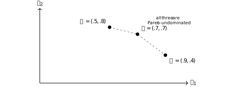
For scalar weights \((0.8,0.2)\), the scores are \(S(A)=0.80\), \(S(B)=0.70\), and \(S(C)=0.56\), so \(A\) wins. The worst-group scores are \(0.4\), \(0.7\), and \(0.5\), so \(B\) wins. No point dominates another coordinatewise, hence the Pareto summary retains all three.
The scalar, Pareto, and worst-group summaries were defined in Definition 4.1.13--Definition 4.1.15. Their non-equivalence is explicit in these three points, while the choice of a social or evaluation rule remains open.
4.2. Evaluation transport and matched protocols [ftip-00F9]AGENTDRAFTED
4.2. Evaluation transport and matched protocols [ftip-00F9]AGENTDRAFTED
This section compares post-training artifacts only through declared evaluation laws, inference protocols, utilities, seeds, and budgets. It proves finite transport statements locally and treats long-horizon research-state records as empirical evidence, not as theorems.
4.2.1. Evaluation laws and couplings [ftip-00FA]AGENTDRAFTED
4.2.1. Evaluation laws and couplings [ftip-00FA]AGENTDRAFTED
Convention 4.2.1.1. A named evaluation experiment [ftip-00FB]AGENTDRAFTED
Convention 4.2.1.1. A named evaluation experiment [ftip-00FB]AGENTDRAFTED
A named evaluation experiment records the artifact, task law, inference protocol, evaluator, seed kernel, budget, and sampling unit. Two reported scores are comparable only after these coordinates and their intended target have been stated.
Definition 4.2.1.2. Evaluation law [ftip-00FC]AGENTDRAFTED
Definition 4.2.1.2. Evaluation law [ftip-00FC]AGENTDRAFTED
For a fixed evaluation interface from Convention 4.1.1, an evaluation law is a probability measure \(\mathsf Q\) on the finite outcome space \(\mathcal Z=\mathcal X_{\mathsf T_{\rm ev}}\times \mathcal O_{\mathsf T_{\rm ev}}\) with random pair \((X,O)\sim \mathsf Q\). Its score for artifact \(M\) is a bounded measurable map \(s_M:\mathcal Z\to [0,1]\). Write \(J_{\mathsf Q}(M)=\mathbb E_{\mathsf Q}[s_M(X,O)]\).
Definition 4.2.1.3. Matched evaluation pair [ftip-00FD]AGENTDRAFTED
Definition 4.2.1.3. Matched evaluation pair [ftip-00FD]AGENTDRAFTED
A matched evaluation pair is \((\mathsf Q,\mathsf I,b,\Lambda )\) and \((\mathsf Q',\mathsf I',b',\Lambda ')\) together with a coupling \((Z,Z')\) whose marginals are the two laws. The pair is matched on the declared coordinates when the task, utility, evaluator version, and sampling unit are shared; any changed coordinate is named.
Definition 4.2.1.4. Paired finite score estimator [ftip-00FE]AGENTDRAFTED
Definition 4.2.1.4. Paired finite score estimator [ftip-00FE]AGENTDRAFTED
For iid coupled draws \((Z_j,Z'_j)_{j=1}^m\), define \(\widehat \Delta _m=m^{-1}\sum _{j=1}^m(s_M(Z_j)-s_{M'}(Z'_j))\). The pairing is part of the estimator specification; it does not silently identify the two evaluation laws.
Theorem 4.2.1.5. Unbiasedness of the paired score estimator [ftip-00FF]AGENTDRAFTED
Theorem 4.2.1.5. Unbiasedness of the paired score estimator [ftip-00FF]AGENTDRAFTED
Under the iid coupling in Definition 4.2.1.4, \(\mathbb E[\widehat \Delta _m]=J_{\mathsf Q}(M)-J_{\mathsf Q'}(M')\).
Proof.
Proof.
Linearity of expectation gives the displayed identity.
\[ \mathbb E[\widehat \Delta _m] =m^{-1}\sum _j\left (\mathbb E[s_M(Z_j)]- \mathbb E[s_{M'}(Z'_j)]\right ). \]The coupling fixes the joint sampling but does not change either marginal, so the two terms are the stated expectations.
Example 4.2.1.6. Common seeds can reduce paired variance [ftip-00G0]AGENTDRAFTED
Example 4.2.1.6. Common seeds can reduce paired variance [ftip-00G0]AGENTDRAFTED
If \(s_M(Z)=s_{M'}(Z')\) almost surely under a common-seed coupling, then \(\widehat \Delta _m=0\) for every sample even when independent sampling would have nonzero variance. This is a variance statement, not evidence that the two artifacts have equal behavior on a different law.
Remark 4.2.1.7. A coupling does not merge estimands [ftip-00G1]AGENTDRAFTED
Remark 4.2.1.7. A coupling does not merge estimands [ftip-00G1]AGENTDRAFTED
The result in Theorem 4.2.1.5 follows from its displayed hypotheses. A shared seed can make a paired comparison precise while the changed task law, evaluator, or inference budget still changes the estimand. No causal effect follows without a declared intervention and matched coordinates.
4.2.2. Utility transport [ftip-00G2]AGENTDRAFTED
4.2.2. Utility transport [ftip-00G2]AGENTDRAFTED
Definition 4.2.2.1. Bounded utility perturbation [ftip-00G3]AGENTDRAFTED
Definition 4.2.2.1. Bounded utility perturbation [ftip-00G3]AGENTDRAFTED
On a common finite outcome law \(\mathsf Q\), let each artifact \(M\) have score maps \(s_M,t_M:\mathcal Z\to [0,1]\). They have perturbation radius \(\varepsilon =\sup _{M,\,z\in \operatorname {supp}(\mathsf Q)} |s_M(z)-t_M(z)|\) when \(0\leq \varepsilon \leq 1\); write \(J_s(M)=\mathbb E_{\mathsf Q}[s_M]\) and \(J_t(M)=\mathbb E_{\mathsf Q}[t_M]\).
Theorem 4.2.2.2. Direct utility transport bound [ftip-00G4]AGENTDRAFTED
Theorem 4.2.2.2. Direct utility transport bound [ftip-00G4]AGENTDRAFTED
Under Definition 4.2.2.1, every artifact \(M\) satisfies \(|J_s(M)-J_t(M)|\leq \varepsilon \).
Proof.
Proof.
Pointwise bounds give \(-\varepsilon \leq s_M(z)-t_M(z)\leq \varepsilon \). Taking expectations preserves both inequalities.
Corollary 4.2.2.3. Transporting an artifact comparison [ftip-00G5]AGENTDRAFTED
Corollary 4.2.2.3. Transporting an artifact comparison [ftip-00G5]AGENTDRAFTED
If two artifacts \(M_1,M_0\) are scored by both \(s\) and \(t\) under the same law and \(\lVert s-t\rVert _{\infty ,\mathsf Q}\leq \varepsilon \), then the gain difference obeys \(|(J_s(M_1)-J_s(M_0))-(J_t(M_1)-J_t(M_0))| \leq 2\varepsilon \). This is a finite utility perturbation bound, not a training or distribution-shift theorem.
Example 4.2.2.4. Equal aggregate score can hide a slice reversal [ftip-00G6]AGENTDRAFTED
Example 4.2.2.4. Equal aggregate score can hide a slice reversal [ftip-00G6]AGENTDRAFTED
On equally likely outcomes \(a,b\), take score vectors \((s_{M_1}(a),s_{M_1}(b))=(1,0)\) and \((s_{M_0}(a),s_{M_0}(b))=(0,1)\); a second score map swaps coordinates. Both artifacts have aggregate score \(1/2\) under both maps, but their per-outcome ordering reverses. Aggregate transport alone does not identify localized behavior.
Remark 4.2.2.5. Common domains are a transport hypothesis [ftip-00G7]AGENTDRAFTED
Remark 4.2.2.5. Common domains are a transport hypothesis [ftip-00G7]AGENTDRAFTED
The bound in Theorem 4.2.2.2 requires the same finite outcome support. Changing prompts, parsers, evaluators, or inference budgets is a new law and must be recorded rather than hidden inside a score perturbation.
4.2.3. Prompt and research-state transport [ftip-00G8]AGENTDRAFTED
4.2.3. Prompt and research-state transport [ftip-00G8]AGENTDRAFTED
Definition 4.2.3.1. Research-state observable [ftip-00G9]AGENTDRAFTED
Definition 4.2.3.1. Research-state observable [ftip-00G9]AGENTDRAFTED
For a finite record space \(\mathcal R\), an observable is a map \(h:\mathcal R\to \mathcal H\). A summary-only evaluator sees \(h(r)\) and not the underlying record \(r\); the omitted coordinates are unavailable to that evaluator.
Definition 4.2.3.2. Compaction kernel [ftip-00GA]AGENTDRAFTED
Definition 4.2.3.2. Compaction kernel [ftip-00GA]AGENTDRAFTED
A compaction kernel is a randomized map \(K(dh\mid r)\) from records in \(\mathcal R\) to summaries in \(\mathcal H\). A deterministic summary is the special case \(K(dh\mid r)=\delta _{h(r)}\).
Theorem 4.2.3.3. Summary-only indistinguishability [ftip-00GB]AGENTDRAFTED
Theorem 4.2.3.3. Summary-only indistinguishability [ftip-00GB]AGENTDRAFTED
Let \(r,r'\in \mathcal R\) induce the same summary law under the kernel in Definition 4.2.3.2. Any randomized decision rule that receives only that summary has the same output law in the two worlds.
Proof.
Proof.
The output law is the pushforward of the common summary law through the same decision kernel. Pushforwards of equal finite measures are equal.
Example 4.2.3.4. An omitted feasibility constraint [ftip-00GC]AGENTDRAFTED
Example 4.2.3.4. An omitted feasibility constraint [ftip-00GC]AGENTDRAFTED
Two research records can share every summary score while one contains a withdrawn lemma and the other contains a feasible proof plan. A summary-only selector therefore chooses identically, although the correct next action differs. This is a finite witness to information loss, not a claim about a particular model.
Remark 4.2.3.5. Long-horizon records are empirical transport evidence [ftip-00GD]AGENTDRAFTED
Remark 4.2.3.5. Long-horizon records are empirical transport evidence [ftip-00GD]AGENTDRAFTED
The case study in [li2026longhorizon], Sections 4--7, reports file-based memory, human steering, and research-state failures under one system and task. It motivates explicit observables and omitted constraints; it does not supply the finite theorem in Theorem 4.2.3.3 or a general model capability law.
4.2.4. Evaluation cells and budget accounting [ftip-00GE]AGENTDRAFTED
4.2.4. Evaluation cells and budget accounting [ftip-00GE]AGENTDRAFTED
Definition 4.2.4.1. Evaluation cell [ftip-00GF]AGENTDRAFTED
Definition 4.2.4.1. Evaluation cell [ftip-00GF]AGENTDRAFTED
An evaluation cell is \(C=(M,\mathsf Q,\mathsf I,b,\Lambda ,v)\), where \(M\) is an artifact, \(\mathsf Q\) a task law, \(\mathsf I\) an inference protocol, \(b\) a budget, \(\Lambda \) a seed kernel, and \(v\) an evaluator version. A cell comparison may differ in named coordinates only.
Lemma 4.2.4.2. Additive evaluation cost [ftip-00GG]AGENTDRAFTED
Lemma 4.2.4.2. Additive evaluation cost [ftip-00GG]AGENTDRAFTED
For a finite evaluation plan with disjoint stages of costs \(c_1,\ldots ,c_k\in \mathbb R_{\geq 0}\), total cost is \(c=\sum _{i=1}^k c_i\). Appending a stage increases cost by its declared amount and cannot preserve a budget \(B\) unless the remaining slack covers it.
Proof.
Proof.
The statement is the associativity and monotonicity of finite sums.
Theorem 4.2.4.3. Budget-preserving matched comparison [ftip-00GH]AGENTDRAFTED
Theorem 4.2.4.3. Budget-preserving matched comparison [ftip-00GH]AGENTDRAFTED
Let two evaluation plans use the same declared stages except for a substitution whose cost is at most the replaced stage cost. If their common prefix cost is \(c_0\) and both suffix costs fit \(B-c_0\), then both cells in Definition 4.2.4.1 are admissible under budget \(B\).
Proof.
Proof.
Apply Lemma 4.2.4.2 to the common prefix and each suffix. The assumed inequalities give total cost at most \(B\) in each plan.
Example 4.2.4.4. Cost-balanced evaluation cells [ftip-00GI]AGENTDRAFTED
Example 4.2.4.4. Cost-balanced evaluation cells [ftip-00GI]AGENTDRAFTED
A paired run can spend \(B=100\) units as 40 units of inference, 20 of evaluator calls, and 40 of audit. Replacing 10 inference units by 10 audit units preserves the budget, but changes the cell and must not be described as the same inference protocol.
Remark 4.2.4.5. Execution and evaluator confounds [ftip-00GJ]AGENTDRAFTED
Remark 4.2.4.5. Execution and evaluator confounds [ftip-00GJ]AGENTDRAFTED
A score change can arise from the artifact, prompt law, inference budget, parser, evaluator version, or execution failure. A matched-cell report names these coordinates before interpreting a paired gain.
4.2.5. Distribution shift and ranking reversals [ftip-00GK]AGENTDRAFTED
4.2.5. Distribution shift and ranking reversals [ftip-00GK]AGENTDRAFTED
Example 4.2.5.1. Train and evaluation laws can reverse a ranking [ftip-00GL]AGENTDRAFTED
Example 4.2.5.1. Train and evaluation laws can reverse a ranking [ftip-00GL]AGENTDRAFTED
Let \(\mathsf Q_{\rm tr}\) put masses \(.9,.1\) on \(a,b\), and let \(\mathsf Q_{\rm ev}\) swap them. Artifacts \(M_1,M_0\) with score vectors \((s_{M_1}(a),s_{M_1}(b))=(1,0)\) and \((s_{M_0}(a),s_{M_0}(b))=(0,1)\) rank oppositely under the two laws. A training score is not an evaluation transport certificate.
Theorem 4.2.5.2. Total-variation transport bound [ftip-00GM]AGENTDRAFTED
Theorem 4.2.5.2. Total-variation transport bound [ftip-00GM]AGENTDRAFTED
For any score \(s:\mathcal Z\to [0,1]\) and finite laws \(\mathsf Q,\mathsf Q'\), \(|\mathbb E_{\mathsf Q}s-\mathbb E_{\mathsf Q'}s|\leq \lVert \mathsf Q-\mathsf Q'\rVert _{\rm TV}\), where \(\lVert \mathsf Q-\mathsf Q'\rVert _{\rm TV}:=\frac 12\sum _{z\in \mathcal Z} |\mathsf Q(z)-\mathsf Q'(z)|\).
Proof.
Proof.
Expand the finite expectation difference and use \(|s(z)|\leq 1\). The positive and negative parts are bounded by the total variation mass, giving the displayed inequality.
Example 4.2.5.3. A sharp two-point transport bound [ftip-00GN]AGENTDRAFTED
Example 4.2.5.3. A sharp two-point transport bound [ftip-00GN]AGENTDRAFTED
On \(\mathcal Z=\{a,b\}\), let \(s(a)=1,s(b)=0\), and let \(\mathsf Q(a)=1\), \(\mathsf Q'(a)=1-\eta \), and \(\mathsf Q'(b)=\eta \). The score difference and total variation distance are both \(\eta \).
Remark 4.2.5.4. What transport does not identify [ftip-00GO]AGENTDRAFTED
Remark 4.2.5.4. What transport does not identify [ftip-00GO]AGENTDRAFTED
The bounds above transport a declared score across a declared law. They do not identify why an artifact changed, establish support expansion, prove generalization, or order different evaluators whose outcome spaces differ.
Example 4.2.5.5. A minimal evaluation trace [ftip-00GP]AGENTDRAFTED
Example 4.2.5.5. A minimal evaluation trace [ftip-00GP]AGENTDRAFTED
A reproducible record is \((M,\mathsf Q,\mathsf I,b,\Lambda ,v,m, \widehat \Delta _m,c)\), listing the cells, sample count, paired estimate, and cost. Replaying this tuple reproduces the estimator target only when the recorded laws and versions remain available.
Remark 4.2.5.6. Execution controls for a matched evaluation [ftip-00GQ]AGENTDRAFTED
Remark 4.2.5.6. Execution controls for a matched evaluation [ftip-00GQ]AGENTDRAFTED
A matched evaluation requires execution gates, contamination checks, grader calibration, and an audit of the result before it is committed. These controls make the comparison auditable; they do not by themselves establish capability acquisition.
4.3. Analytical questions and falsifiers [ftip-005T]AGENTDRAFTED
4.3. Analytical questions and falsifiers [ftip-005T]AGENTDRAFTED
Successful support, verifier error, and entropy statistics distinguish properties that a benchmark summary can combine. Finite examples and counterexamples distinguish these quantities.
Definition 4.3.1. Successful-support probability [ftip-005U]AGENTDRAFTED
Definition 4.3.1. Successful-support probability [ftip-005U]AGENTDRAFTED
Fix the evaluation interface and success threshold \(u_*\) from Convention 4.1.1. For a protocol \(P\) and instance \(x\in \mathcal X_{\mathsf T_{\rm ev}}\), its successful-support probability is
\[ p_P(x) =\Pr \left [ U\left (x,\mathsf {Eval}_b(M_P,x;\Xi );\Omega \right )\geq u_* \right ]. \]The probability includes protocol, inference, environment, and evaluator randomness: \(M_P\) is drawn from the protocol, while \((\Xi ,\Omega )\) is drawn from \(\Lambda _{\rm ev}(\cdot \mid x)\) independently of training. The quantity is instance-specific and budget-specific.
Definition 4.3.2. Successful-support coverage [ftip-005V]AGENTDRAFTED
Definition 4.3.2. Successful-support coverage [ftip-005V]AGENTDRAFTED
For threshold \(0<\alpha \leq 1\), the successful-support coverage of protocol \(P\) under evaluation law \(Q_{\rm ev}\) is
\[ \operatorname {Cov}_\alpha (P) =Q_{\rm ev}\left (\{x:p_P(x)\geq \alpha \}\right ). \]Coverage records how much task mass has at least the declared success probability. It does not average the probabilities above or below the threshold.
Remark 4.3.3. Task-level success and coverage [ftip-005W]AGENTDRAFTED
Remark 4.3.3. Task-level success and coverage [ftip-005W]AGENTDRAFTED
Increasing probability mass on known solutions need not increase coverage of the task family. Pass-at-\(k\) and related support-sensitive measurements motivate this distinction. Sections 3--5 of Does reinforcement learning really incentivize reasoning capacity in LLMs beyond the base model?[yue2025does] and Sections 2--3 of Understanding r1-zero-like training: A critical perspective[liu2025understanding] compare post-training behavior with base-model support and discuss why response accuracy alone may overstate what RL creates beyond a base model.
The threshold \(\alpha \), inference budget, task law, and success predicate must all be reported. Finite samples estimate this quantity; they do not reveal the unobserved tail without assumptions.
Definition 4.3.4. Uniform task-family acquisition witness [ftip-005X]AGENTDRAFTED
Definition 4.3.4. Uniform task-family acquisition witness [ftip-005X]AGENTDRAFTED
Fix a finite, independently selected family \(G\subseteq \mathcal X_{\mathsf T_{\rm ev}}\), thresholds \(0\leq \alpha <\beta \leq 1\), and the common evaluation interface of Convention 4.1.1. Protocols \(P_0\) and \(P_1\) have a uniform task-family acquisition witness on \(G\) when
\[ p_{P_0}(x)\leq \alpha \quad \hbox {and}\quad p_{P_1}(x)\geq \beta \qquad \text {for every }x\in G. \]For each \(x\), the successful event in Definition 4.3.1 supplies the fixed-budget transfer event in Definition 1.1.5. The displayed inequalities specialize that earlier acquisition witness with \(\varepsilon _0=\alpha \) and \(\varepsilon _1=\beta \), then require the specialization uniformly over \(G\).
Remark 4.3.5. Acquisition evidence across a fixed task family [ftip-005Y]AGENTDRAFTED
Remark 4.3.5. Acquisition evidence across a fixed task family [ftip-005Y]AGENTDRAFTED
The proposed family-level criterion is a demanding paired comparison. The task family and evaluator are fixed independently, and both protocols use the same inference budget. It is stronger than one acquisition witness because the threshold change must hold for every member of \(G\).
A theorem may strengthen the witness with confidence bounds, transfer to a predeclared related family, or a lower bound on newly successful support. Each strengthening requires additional sampling or structural assumptions.
Definition 4.3.6. Verifier error rates [ftip-005Z]AGENTDRAFTED
Definition 4.3.6. Verifier error rates [ftip-005Z]AGENTDRAFTED
Let \(S\in \{0,1\}\) be an independently defined success label and \(A\in \{0,1\}\) the verifier's accept decision on the same outcome. The false-accept and false-reject rates are
\[ \eta _+=\Pr (A=1\mid S=0), \qquad \eta _-=\Pr (A=0\mid S=1). \]Both rates are conditional on the task and outcome distribution used for the audit. They are undefined when the conditioning event has probability zero.
Remark 4.3.7. Verifier error under an independent audit law [ftip-0061]AGENTDRAFTED
Remark 4.3.7. Verifier error under an independent audit law [ftip-0061]AGENTDRAFTED
Verifier error is measured against an independent success label because a training reward cannot audit itself. The verifier and evidence interfaces are in Definition 2.9.4--Definition 2.9.7. DeepSeek-Prover-V2 [ren2025deepseekproverv2, Section 2.3, ``Reinforcement Learning''] supplies a proof-checking instance. The false-accept/false-reject decomposition is a binary measurement model.
The rates may vary by task, policy, trajectory length, and adversarial pressure. A low average error rate need not prevent reward hacking on the subpopulation favored by optimization.
Example 4.3.8. Reward hacking under an incomplete checker [ftip-0060]AGENTDRAFTED
Example 4.3.8. Reward hacking under an incomplete checker [ftip-0060]AGENTDRAFTED
Shifting probability mass toward a checker exploit raises proxy reward while reducing independently judged utility.
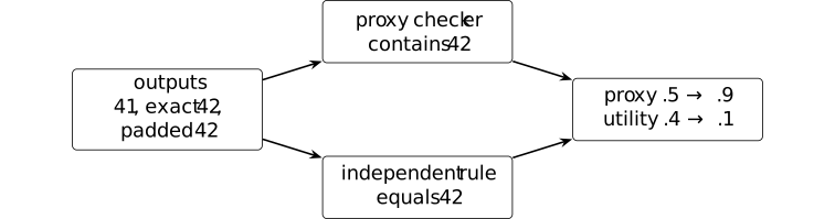
Let the three outputs be \(y_0=\text {41}\), \(y_1=\text {42}\), and \(y_2=\text {ignore; 42; done}\). The proxy accepts \(y_1,y_2\); the independent evaluator accepts only \(y_1\). Moving their probabilities from \((0.5,0.4,0.1)\) to \((0.1,0.1,0.8)\) changes expected proxy reward from \(0.5\) to \(0.9\), but true utility from \(0.4\) to \(0.1\).
Reward exploitation in formal verification is discussed in [ren2025deepseekproverv2, Section 3.2]. The constructed checker exposes one failure mechanism. It provides no basis for treating every executable verifier as incomplete or every proxy improvement as reward hacking.
Definition 4.3.9. Global policy entropy [ftip-0062]AGENTDRAFTED
Definition 4.3.9. Global policy entropy [ftip-0062]AGENTDRAFTED
Fix a finite action space, a finite horizon \(T\), and a declared distribution \(\mu _t\) over public histories at each position. The global policy entropy is the weighted average
\[ H_{\rm global}(\pi ) =\frac 1T\sum _{t=0}^{T-1} \mathbb E_{\mathsf H_t\sim \mu _t} \left [-\sum _a\pi (a\mid \mathsf H_t) \log \pi (a\mid \mathsf H_t)\right ]. \]The history distribution and action alphabet are part of the statistic.
We use the convention \(0\log 0=0\) in this and the following position-entropy formula.
Definition 4.3.10. Token-position entropy [ftip-0063]AGENTDRAFTED
Definition 4.3.10. Token-position entropy [ftip-0063]AGENTDRAFTED
Let \(T_{\rm tok}\) be the random number of generated tokens. For a one-based token position \(t\) satisfying \(\Pr (T_{\rm tok}\geq t)>0\), condition on \(T_{\rm tok}\geq t\) and let \(\xi _t\) be the token. The token-position entropy is
\[ H_t^{\rm pos} =-\sum _{v\in \mathcal V} \Pr (\xi _t=v\mid T_{\rm tok}\geq t) \log \Pr (\xi _t=v\mid T_{\rm tok}\geq t). \]This is the entropy of a position marginal. It is generally different from the history-conditioned entropy averaged in Definition 4.3.9.
Definition 4.3.11. selected-token surprisal [shannon1948mathematical, Part I, Section 6] [ftip-0064]AGENTDRAFTED
Definition 4.3.11. selected-token surprisal [shannon1948mathematical, Part I, Section 6] [ftip-0064]AGENTDRAFTED
For a sampled token \(\xi _t\) under next-token law \(\pi (\,\cdot \mid \mathsf H_t)\), its surprisal is
\[-\log \pi (\xi _t\mid \mathsf H_t).\]It is a random value attached to the selected token. Its conditional expectation over the token equals the finite Shannon entropy of the next-token law.
Remark 4.3.12. Why the entropy statistics are not interchangeable [ftip-0065]AGENTDRAFTED
Remark 4.3.12. Why the entropy statistics are not interchangeable [ftip-0065]AGENTDRAFTED
Shannon's finite entropy A mathematical theory of communication[shannon1948mathematical] can be aggregated over different random objects. Global and position-level entropy statistics use different laws. Selected-token surprisal is a sample statistic, while the other two are expectations under declared history or position laws.
A training intervention can raise one quantity while lowering another. Later claims about exploration or collapse must name the statistic, sampling law, horizon, and conditioning event.
Definition 4.3.13. empirical squared-ratio excess [miao2026when, Theorem 2] [ftip-0066]AGENTDRAFTED
Definition 4.3.13. empirical squared-ratio excess [miao2026when, Theorem 2] [ftip-0066]AGENTDRAFTED
For token-level current-to-behavior ratios \(r_1,\ldots ,r_T\), DGG defines
\[\widehat \chi ^2=\frac 1T\sum _{i=1}^T(r_i^2-1).\]The source relates this statistic to an upper bound on language-model-head gradient energy through a batch-dependent constant. In a finite batch \(\widehat \chi ^2\) can be negative, so it is not automatically a nonnegative empirical Pearson divergence. The result also gives no converse from a small batch gradient to small policy shift.
Example 4.3.14. Lifecycle compute allocation and a finite rollout observation bound [ftip-0067]AGENTDRAFTED
Example 4.3.14. Lifecycle compute allocation and a finite rollout observation bound [ftip-0067]AGENTDRAFTED
A componentwise lifecycle allocation separates resource accounting from the finite number of rollouts available for observation.
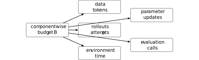
In the coordinate order of Definition 4.1.5, declare a lifecycle budget vector \(\mathbf B\). Its rollout coordinate permits \(N\) attempts. If each attempt has declared success probability \(p\), then \[ \Pr (\text {at least one success})=1-(1-p)^N\leq Np. \] Only the rollout coordinate enters this calculation; no sum or conversion among heterogeneous coordinates is defined.
The finite bound is the union bound applied to Bernoulli rollouts; finite-horizon success probabilities are standard policy-evaluation objects in [sutton2018reinforcement, Section 3.5]. Independence is needed only for the displayed exact expression. The budget vector is illustrative: neither empirical optimality nor interchangeability of heterogeneous units is inferred from it.
Remark 4.3.15. Finite questions and necessary assumptions [ftip-0068]AGENTDRAFTED
Remark 4.3.15. Finite questions and necessary assumptions [ftip-0068]AGENTDRAFTED
Finite analysis raises three questions: how conditional success rates bound long-horizon success, how replay-ratio concentration controls update error, and how trajectory extrapolation with periodic recovery affects evaluation regret. A cost comparison also depends on rollout, update, environment, storage, and evaluation work.
Finite counterexamples show why these questions need additional assumptions. Finite policies can separate the entropy statistics above. Two verifiers can agree on all observed training records yet differ on an unobserved adversarial region. Two parameter paths can share early low-rank summaries and diverge after a new successful rollout. These examples mark where additional assumptions are unavoidable.
The DGG and NExt papers motivate reuse and trajectory-compression hypotheses but do not establish these general results. Bounds on update error and extrapolation regret require assumptions relating the monitored quantities to the corresponding outcomes.
4.4. Finite consequences and obstructions [ftip-0075]AGENTDRAFTED
4.4. Finite consequences and obstructions [ftip-0075]AGENTDRAFTED
This section turns parts of the preceding setup into finite mathematical statements. The results concern declared probability spaces, finite decision sets, recorded feedback, or explicitly stated matrix models. They do not by themselves establish a scaling law for language-model capability.
We begin with discovery and support, then study proxy rewards and verifiers. The third subsection asks what can be learned from a fixed feedback transcript. The last subsection studies the DGG inequalities before introducing trajectory-compression diagnostics and counterexamples.
4.4.1. Finite discovery and support [ftip-0076]AGENTDRAFTED
4.4.1. Finite discovery and support [ftip-0076]AGENTDRAFTED
A successful continuation can have positive probability and still be difficult to observe within a finite rollout budget. This subsection separates the probability of observing a success from support, coverage, and capability acquisition.
Convention 4.4.1.1. Repeated attempts and the discovery event [ftip-0077]AGENTDRAFTED
Convention 4.4.1.1. Repeated attempts and the discovery event [ftip-0077]AGENTDRAFTED
Fix a task instance, evaluator, success threshold, and a joint law for \(B\geq 1\) attempts. Let \(E_i\) be the event that attempt \(i\) succeeds. The discovery event by attempt \(B\) is
\[ D_B=\bigcup _{i=1}^{B}E_i. \]Write \(p_i=\Pr (E_i)\). Independence is an additional property of the declared joint law; it is not implied by repeated decoding, a shared model, or a common environment. In the independent and identically distributed case, write \(p_i=p\). When the attempt law is the one fixed in Definition 4.3.1, this \(p\) is the corresponding successful-support probability.
Theorem 4.4.1.2. Discovery under independent attempts [ftip-0078]AGENTDRAFTED
Theorem 4.4.1.2. Discovery under independent attempts [ftip-0078]AGENTDRAFTED
Assume the events \(E_1,\ldots ,E_B\) of Convention 4.4.1.1 are independent. Then
\[ \Pr (D_B)=1-\prod _{i=1}^{B}(1-p_i). \]In particular, independent attempts with a common success probability \(p\) satisfy
\[ \Pr (D_B)=1-(1-p)^B. \]
Proof.
Proof.
The complement of discovery is \(D_B^{\mathsf c}=\bigcap _{i=1}^{B}E_i^{\mathsf c}\). Independence gives \(\Pr (D_B^{\mathsf c})=\prod _i\Pr (E_i^{\mathsf c}) =\prod _i(1-p_i)\). Taking complements proves the first identity; substituting \(p_i=p\) proves the specialization.
This finite statement follows from the displayed hypotheses. The calculation in Example 4.3.14 is its ten-attempt numerical preview.
Corollary 4.4.1.3. A rollout budget for target discovery probability [ftip-0079]AGENTDRAFTED
Corollary 4.4.1.3. A rollout budget for target discovery probability [ftip-0079]AGENTDRAFTED
This is a finite corollary of Theorem 4.4.1.2, obtained from its displayed hypotheses.
Let \(0<\delta <1\). Under the independent and identically distributed setup of Theorem 4.4.1.2, suppose first that \(0<p<1\). The least positive integer budget whose discovery failure probability is at most \(\delta \) is
\[ B_{\min } =\left \lceil \frac {\log \delta }{\log (1-p)}\right \rceil . \]If \(p=0\), no finite positive budget reaches failure probability below one. If \(p=1\), one attempt suffices.
Proof.
Proof.
For \(0<p<1\), Theorem 4.4.1.2 gives failure probability \((1-p)^B\). The inequality \((1-p)^B\leq \delta \) is equivalent to \(B\geq \frac {\log \delta }{\log (1-p)}\) because both logarithms are negative. The least integer solution is the displayed ceiling. The two boundary cases follow directly from \((1-p)^B\).
Lemma 4.4.1.4. Discovery bounds from conditional success rates [ftip-007A]AGENTDRAFTED
Lemma 4.4.1.4. Discovery bounds from conditional success rates [ftip-007A]AGENTDRAFTED
Put \(D_0=\varnothing \). Whenever \(\Pr (D_{i-1}^{\mathsf c})>0\), define the surviving conditional success rate
\[ q_i=\Pr (E_i\mid D_{i-1}^{\mathsf c}). \]If these rates are defined through step \(B\), then
\[ \Pr (D_B^{\mathsf c})=\prod _{i=1}^{B}(1-q_i). \]Consequently, if \(0\leq \underline q\leq q_i\leq \overline q\leq 1\) for every surviving step, then
\[ 1-(1-\underline q)^B \leq \Pr (D_B) \leq 1-(1-\overline q)^B. \]
Proof.
Proof.
The chain rule gives \(\Pr (D_i^{\mathsf c})=\Pr (D_{i-1}^{\mathsf c})(1-q_i)\). Iteration proves the product identity, and the coordinatewise bounds on \(1-q_i\) give the two discovery bounds.
No independence assumption is used. The conditional rates may change with the earlier failures, an adaptive decoder, or a changing environment state.
This finite statement follows from the displayed hypotheses.
Remark 4.4.1.5. Discovery is neither acquisition nor coverage [ftip-007B]AGENTDRAFTED
Remark 4.4.1.5. Discovery is neither acquisition nor coverage [ftip-007B]AGENTDRAFTED
The discovery event concerns whether a declared sampling procedure observes at least one success. Increasing its probability can be an elicitation effect in the sense of Definition 1.1.3: more attempts expose behaviour that already had positive probability. It is not by itself the independent before--after comparison required by Definition 1.1.5.
Successful-support coverage in Definition 4.3.2 integrates an instance-level threshold over a task law. A large discovery probability on one instance therefore does not establish broad coverage or the uniform task-family witness of Definition 4.3.4.
Theorem 4.4.1.6. Finite exponential tilting preserves support [ftip-007C]AGENTDRAFTED
Theorem 4.4.1.6. Finite exponential tilting preserves support [ftip-007C]AGENTDRAFTED
Fix a prompt \(x\), a finite response set \(\mathcal Y\), a reference policy \(\pi _{\mathrm {ref}}\), a finite real reward \(r(x,y)\), and \(\beta >0\). Let \(\pi _r\) be the normalized exponential tilt of Definition 2.7.3. Then, for every \(y\in \mathcal Y\),
\[ \pi _r(y\mid x)>0 \quad \Longleftrightarrow \quad \pi _{\mathrm {ref}}(y\mid x)>0. \]
Proof.
Proof.
The multiplier \(\exp (r(x,y)/\beta )\) is finite and strictly positive. The finite normalizer \(Z_r(x)\) is also strictly positive. Multiplication by the first quantity and division by the second therefore preserve whether the reference mass is zero or positive.
The source policy form appears as equation (4) in [rafailov2023direct, Section 4]; the displayed result is the finite corollary derived here. Infinite rewards, non-normalizable response spaces, approximate optimization, and changes to the generation mechanism lie outside the statement.
Remark 4.4.1.7. Formal support and operational discoverability [ftip-007D]AGENTDRAFTED
Remark 4.4.1.7. Formal support and operational discoverability [ftip-007D]AGENTDRAFTED
Support preservation is a statement about exact positive probability. A response can remain in mathematical support while its mass becomes too small to observe within the available rollout budget. The identities in Theorem 4.4.1.2 and Corollary 4.4.1.3 quantify this distinction for declared independent attempts.
Top-\(k\) truncation, nucleus sampling, finite numerical precision, context limits, and parser constraints can also remove an operational route even when the underlying softmax law assigns it positive mass. Claims about elicitation must therefore name both the policy law and the executable inference procedure.
Example 4.4.1.8. Counterexample: Equal one-shot success, unequal successful coverage [ftip-007E]AGENTDRAFTED
Example 4.4.1.8. Counterexample: Equal one-shot success, unequal successful coverage [ftip-007E]AGENTDRAFTED
Let the evaluation law be uniform on two instances \(x_1,x_2\). Consider protocols \(P\) and \(P'\) with successful-support probabilities
\[ \bigl (p_P(x_1),p_P(x_2)\bigr ) =\left (\frac 12,\frac 12\right ), \qquad \bigl (p_{P'}(x_1),p_{P'}(x_2)\bigr ) =(1,0). \]Both protocols have mean one-shot success \(1/2\). At threshold \(\alpha =1/2\), however, Definition 4.3.2 gives
\[ \operatorname {Cov}_{1/2}(P)=1, \qquad \operatorname {Cov}_{1/2}(P')=\frac 12. \]Thus average success does not determine successful-support coverage. The example is finite and uses the same task law and threshold for both protocols; it does not compare their training costs or establish acquisition.
4.4.2. Proxy reward and verifier fidelity [ftip-007F]AGENTDRAFTED
4.4.2. Proxy reward and verifier fidelity [ftip-007F]AGENTDRAFTED
A proxy can guide an update or rank sampled candidates without agreeing with the independently declared utility of the resulting output. This subsection separates pointwise proxy error from average error under a shifted law. It then distinguishes repeated false-accept events from the output of a candidate selector. Pointwise approximation and explicit probability assumptions support different guarantees; an average audit number alone supplies neither.
Definition 4.4.2.1. Uniform proxy approximation [ftip-007G]AGENTDRAFTED
Definition 4.4.2.1. Uniform proxy approximation [ftip-007G]AGENTDRAFTED
Let \(\mathcal Y_0\) be a nonempty finite set of candidate outcomes. Let \(U:\mathcal Y_0\to \mathbb R\) be an independently declared utility and \(\widehat U:\mathcal Y_0\to \mathbb R\) a proxy score. The proxy is a uniform approximation to \(U\) on \(\mathcal Y_0\) with error \(\varepsilon \) when \(\varepsilon \geq 0\) and
\[ \sup _{y\in \mathcal Y_0}\lvert \widehat U(y)-U(y)\rvert \leq \varepsilon . \]The candidate set is part of the claim. Approximation on training outcomes, on one policy's support, or in expectation is not uniform approximation on a larger set reached after optimization.
Theorem 4.4.2.2. Uniform proxy error gives two-epsilon selection regret [ftip-007H]AGENTDRAFTED
Theorem 4.4.2.2. Uniform proxy error gives two-epsilon selection regret [ftip-007H]AGENTDRAFTED
Under the conditions of Definition 4.4.2.1, choose
\[ y^\star \in \operatorname *{arg\,max}_{y\in \mathcal Y_0}U(y), \qquad \widehat y\in \operatorname *{arg\,max}_{y\in \mathcal Y_0}\widehat U(y). \]Then the utility regret of selecting by the proxy satisfies
\[ 0\leq U(y^\star )-U(\widehat y)\leq 2\varepsilon . \]
Proof.
Proof.
Optimality of \(\widehat y\) for the proxy and the two pointwise error bounds give
\[ \begin {aligned} U(y^\star ) &\leq \widehat U(y^\star )+\varepsilon \\ &\leq \widehat U(\widehat y)+\varepsilon \\ &\leq U(\widehat y)+2\varepsilon . \end {aligned} \]Optimality of \(y^\star \) for \(U\) gives the lower bound.
This finite statement follows from the displayed hypotheses.
Remark 4.4.2.3. The two-epsilon theorem is a decision bound [ftip-007I]AGENTDRAFTED
Remark 4.4.2.3. The two-epsilon theorem is a decision bound [ftip-007I]AGENTDRAFTED
The bound in Theorem 4.4.2.2 follows directly from the uniform approximation condition. It compares two maximizers on one fixed finite candidate set. It does not describe how either score was learned or how a policy changes when that score becomes a training objective.
The result is useful because its transfer assumption is visible. To apply it after an update or a larger search, the uniform bound must hold on the outcomes that the new procedure can actually select. The verifier evidence of Definition 2.9.5 can support such an audit, but reproducible evidence alone does not establish the bound.
Example 4.4.2.4. Counterexample: Small average proxy error fails after distribution shift [ftip-007J]AGENTDRAFTED
Example 4.4.2.4. Counterexample: Small average proxy error fails after distribution shift [ftip-007J]AGENTDRAFTED
Let the finite decision set be \(\mathcal Y_0=\{y_{\rm safe},y_{\rm exploit}\}\). Define its utility and proxy utility by the following table.
\[ \begin {array}{c|cc} &y_{\rm safe}&y_{\rm exploit}\\ \hline U&1&0\\ \widehat U&1&2. \end {array} \]For \(0<\delta <1\), let a reference law \(P_\delta \) assign probability \(\delta \) to \(y_{\rm exploit}\). Its mean absolute proxy error is
\[ \mathbb E_{P_\delta }\lvert \widehat U-U\rvert =2\delta , \]which tends to zero with \(\delta \). Nevertheless, proxy maximization selects \(y_{\rm exploit}\) and incurs utility regret \(1\). Under the shifted law concentrated on that selected outcome, the mean error is \(2\). Thus no vanishing selection-regret bound can depend only on average error under the reference law.
This two-outcome construction isolates the distribution-shift warning in Remark 4.3.7. It does not claim that a particular learned verifier has this error profile; Example 4.3.8 gives a source-linked checker instance with the same proxy-versus-utility separation.
Definition 4.4.2.5. Repeated verifier audit [ftip-007K]AGENTDRAFTED
Definition 4.4.2.5. Repeated verifier audit [ftip-007K]AGENTDRAFTED
A repeated verifier audit of size \(N\geq 1\) records pairs \((S_i,A_i)\in \{0,1\}^2\) for candidates \(1\leq i\leq N\). Here \(S_i\) is an independently defined success label and \(A_i\) is the verifier decision, as in Definition 4.3.6. Define
\[ C_i^{\rm fa}=\{S_i=0,\ A_i=1\}, \qquad \mathcal E_N^{\rm fa}=\bigcup _{i=1}^N C_i^{\rm fa}. \]The event \(\mathcal E_N^{\rm fa}\) says that at least one invalid candidate was accepted. It does not say which candidate a downstream selector returns. Write \(\phi _i=\Pr (C_i^{\rm fa})\). When \(\iota _i=\Pr (S_i=0)>0\), the conditional false-accept rate \(\eta _{+,i}=\Pr (A_i=1\mid S_i=0)\) is defined and \(\phi _i=\iota _i\eta _{+,i}\).
Theorem 4.4.2.6. Independent false accepts amplify with candidate count [ftip-007L]AGENTDRAFTED
Theorem 4.4.2.6. Independent false accepts amplify with candidate count [ftip-007L]AGENTDRAFTED
In the repeated audit of Definition 4.4.2.5, suppose the pairs \((S_i,A_i)\) are independent and identically distributed. Assume
\[ \iota =\Pr (S_i=0)>0, \qquad \eta _+=\Pr (A_i=1\mid S_i=0). \]Then the probability that at least one accepted invalid candidate exists among the \(N\) audited candidates is
\[ \Pr (\mathcal E_N^{\rm fa})=1-(1-\iota \eta _+)^N. \]It is strictly increasing in \(N\) when \(0<\iota \eta _+<1\), and it converges to \(1\) when \(\iota \eta _+>0\).
Proof.
Proof.
Each \(C_i^{\rm fa}\) has probability \(\iota \eta _+\). Independence of the audited pairs makes the events \(C_i^{\rm fa}\) independent. Therefore
\[ \Pr \left ((\mathcal E_N^{\rm fa})^c\right ) =\Pr \left (\bigcap _{i=1}^N (C_i^{\rm fa})^c\right ) =\prod _{i=1}^N(1-\iota \eta _+) =(1-\iota \eta _+)^N. \]Taking complements gives the equality. The monotonicity and limit follow from the elementary powers of \(1-\iota \eta _+\).
This finite statement follows from the displayed hypotheses.
Theorem 4.4.2.7. A false-accept union bound without independence [ftip-007M]AGENTDRAFTED
Theorem 4.4.2.7. A false-accept union bound without independence [ftip-007M]AGENTDRAFTED
For any joint law of a repeated verifier audit,
\[ \Pr (\mathcal E_N^{\rm fa})\leq \sum _{i=1}^N \phi _i. \]If \(\iota _i=\Pr (S_i=0)>0\) for every \(i\), this becomes
\[ \Pr (\mathcal E_N^{\rm fa})\leq \sum _{i=1}^N \iota _i\eta _{+,i}. \]
Proof.
Proof.
Apply the union bound to \(\mathcal E_N^{\rm fa}=\bigcup _i C_i^{\rm fa}\). The factorization \(\phi _i=\iota _i\eta _{+,i}\) follows from conditional probability whenever \(\iota _i>0\). If \(\iota _i=0\), then \(\phi _i=0\) while the corresponding conditional rate is undefined, so the first display remains the unconditional statement.
Without a dependence assumption, matching marginal error rates do not give the equality in Theorem 4.4.2.6; the events \(C_i^{\rm fa}\) could coincide.
This finite statement follows from the displayed hypotheses.
Example 4.4.2.8. Weight updates and candidate selection are different proxy operators [ftip-007N]AGENTDRAFTED
Example 4.4.2.8. Weight updates and candidate selection are different proxy operators [ftip-007N]AGENTDRAFTED
A proxy score can enter a training operator or a selection operator. In the first route it changes the policy; in the second it ranks a finite sample from a policy whose weights remain fixed.
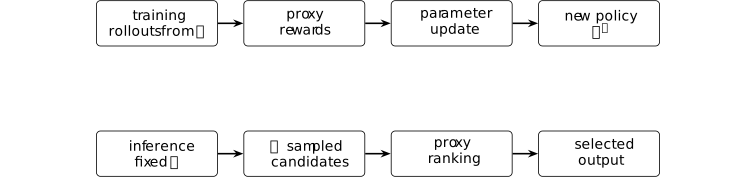
The lifecycle accounting of Definition 4.1.5 places the first route's rollout and update work in separate coordinates. The second route incurs rollout and evaluation work but no parameter update. Consequently, the event \(\mathcal E_N^{\rm fa}\) in Definition 4.4.2.5 concerns the candidate set presented to selection; it is not a claim about the selected output or a training-time policy change.
Remark 4.4.2.9. What verifier error rates do not identify [ftip-007O]AGENTDRAFTED
Remark 4.4.2.9. What verifier error rates do not identify [ftip-007O]AGENTDRAFTED
The rates in Definition 4.3.6 are properties of a declared audit law. They do not identify where errors occur within the task family, how error events depend across repeated candidates, or which accepted candidate a selector returns. Theorem 4.4.2.6 adds identical marginals and independence; Theorem 4.4.2.7 retains only the union bound.
Nor do these rates determine the effect of optimizing against the verifier. That effect depends on how the induced policy or selection law moves mass toward particular outcomes. The incomplete-checker example Example 4.3.8 demonstrates one such movement, while Example 4.4.2.4 shows why an average reference-law error cannot rule it out. These are local finite statements. Any claim about a named verifier still requires its own audit distribution, evidence, and transfer argument.
The deterministic regret lemma Theorem 4.4.2.2, the independent-audit identity Theorem 4.4.2.6, and the union bound Theorem 4.4.2.7 follow from uniform approximation, independent trials, and subadditivity, respectively. Their hypotheses need not hold for a verifier chosen only for its empirical performance.
4.4.3. Feedback identifiability and fixed records [ftip-007P]AGENTDRAFTED
4.4.3. Feedback identifiability and fixed records [ftip-007P]AGENTDRAFTED
A training protocol can respond only to distinctions present in its observations. The following finite setup makes that restriction precise before considering stronger, model-specific limits on preference data.
Definition 4.4.3.1. Finite declared feedback protocol [ftip-007Q]AGENTDRAFTED
Definition 4.4.3.1. Finite declared feedback protocol [ftip-007Q]AGENTDRAFTED
Fix a horizon \(N\geq 0\), finite action sets \(\mathcal A_n\), finite feedback sets \(\mathcal F_n\), and a finite internal-seed set \(\mathcal U\) with a declared law \(\lambda \). A finite declared protocol \(\mathsf P\) consists of selection maps
\[ a_n:\mathcal U\times \prod _{j<n}(\mathcal A_j\times \mathcal F_j) \longrightarrow \mathcal A_n \qquad (0\leq n<N). \]An action may specify the task, rollout record, feedback request, or sampling choice made at that round. The protocol can depend on earlier exposed feedback and its declared seed, but it cannot depend on a latent world field that has not entered those arguments.
Definition 4.4.3.2. Finite feedback world [ftip-008C]AGENTDRAFTED
Definition 4.4.3.2. Finite feedback world [ftip-008C]AGENTDRAFTED
For the action and feedback sets of Definition 4.4.3.1, a finite feedback world \(w\) supplies, for each round \(0\leq n<N\), a probability kernel \(K_{n,w}\) from a generic action--feedback history \((a_0,f_0,\ldots ,a_n)\) ending in \(a_n\in \mathcal A_n\) to \(\mathcal F_n\). Thus, whenever \(a_j\in \mathcal A_j\) and \(f_j\in \mathcal F_j\),
\[ K_{n,w}(\,\cdot \mid a_0,f_0,\ldots ,a_n) \in \Delta (\mathcal F_n). \]Two worlds may agree on every feedback kernel queried by a protocol while differing in latent utility, unrequested labels, or unobserved environment facts. Those latent fields are not feedback until a declared query exposes them.
Definition 4.4.3.3. Observed feedback transcript [ftip-008D]AGENTDRAFTED
Definition 4.4.3.3. Observed feedback transcript [ftip-008D]AGENTDRAFTED
Fix a finite declared protocol \(\mathsf P\) from Definition 4.4.3.1 and a finite feedback world \(w\) from Definition 4.4.3.2. Draw \(U\sim \lambda \) and, for \(0\leq n<N\), set
\[ \begin {aligned} A_n&=a_n(U,A_0,F_0,\ldots ,A_{n-1},F_{n-1}),\\ F_n&\sim K_{n,w}(\,\cdot \mid A_0,F_0,\ldots ,A_n). \end {aligned} \]The resulting observed feedback transcript is
\[ T_w^{\mathsf P}=(U,A_0,F_0,\ldots ,A_{N-1},F_{N-1}). \]All protocol randomness is included in \(U\). Immutable rollout records and typed feedback events may be components of the finite action and feedback sets, as in Definition 2.11.3 and Definition 2.11.5.
Definition 4.4.3.4. Observational equivalence for a declared protocol [ftip-007R]AGENTDRAFTED
Definition 4.4.3.4. Observational equivalence for a declared protocol [ftip-007R]AGENTDRAFTED
Let \(\mathcal T_{\mathsf P}\) be the finite set of possible transcripts for a declared protocol \(\mathsf P\). Two feedback worlds \(w_0,w_1\) are observationally equivalent for \(\mathsf P\), written \(w_0\equiv _{\mathsf P}w_1\), when
\[ \Pr (T_{w_0}^{\mathsf P}=t)=\Pr (T_{w_1}^{\mathsf P}=t) \qquad \text {for every }t\in \mathcal T_{\mathsf P}. \]The relation is protocol-relative. Another protocol may issue a different feedback request and thereby separate the same worlds. Equality only on the realized transcript is weaker than this definition, which compares the whole finite transcript law.
Theorem 4.4.3.5. Post-training cannot distinguish observationally equivalent worlds [ftip-007S]AGENTDRAFTED
Theorem 4.4.3.5. Post-training cannot distinguish observationally equivalent worlds [ftip-007S]AGENTDRAFTED
For a finite random variable \(X\), write \(\operatorname {Law}(X)\) for its probability law. If \(h\) maps the value space of \(X\) to a finite set \(\mathcal Y\), its pushforward law \(h_{\#}\operatorname {Law}(X)\) is characterized by \[ \bigl (h_{\#}\operatorname {Law}(X)\bigr )(\{y\}) =\Pr (h(X)=y),\qquad y\in \mathcal Y. \]
Let \(w_0\equiv _{\mathsf P}w_1\). For any finite output set \(\mathcal Y\) and any readout \(h:\mathcal T_{\mathsf P}\to \mathcal Y\),
\[ h_{\#}\operatorname {Law}(T_{w_0}^{\mathsf P}) =h_{\#}\operatorname {Law}(T_{w_1}^{\mathsf P}). \]Thus a final artifact stamp, update decision, or test chosen solely from the declared protocol's transcript has the same distribution in both worlds.
Proof.
Proof.
For every \(y\in \mathcal Y\), finiteness gives
\[ \begin {aligned} \Pr \left (h(T_{w_0}^{\mathsf P})=y\right ) &=\sum _{\substack {t\in \mathcal T_{\mathsf P}\\h(t)=y}} \Pr (T_{w_0}^{\mathsf P}=t)\\ &=\sum _{\substack {t\in \mathcal T_{\mathsf P}\\h(t)=y}} \Pr (T_{w_1}^{\mathsf P}=t) =\Pr \left (h(T_{w_1}^{\mathsf P})=y\right ). \end {aligned} \]The middle equality is observational equivalence from Definition 4.4.3.4. These point probabilities determine the two pushforward laws.
This finite statement follows from the displayed hypotheses.
Remark 4.4.3.6. A no-free-feedback result, not a no-learning result [ftip-007T]AGENTDRAFTED
Remark 4.4.3.6. A no-free-feedback result, not a no-learning result [ftip-007T]AGENTDRAFTED
Theorem 4.4.3.5 says that the declared observations supply no information that distinguishes \(w_0\) from \(w_1\). It does not say that the output must equal the initial model, that the parameters cannot change, or that performance cannot improve in both worlds. Pretraining, inductive bias, computation on the observed records, and generalization may still produce an improvement shared by the two worlds.
Calling the theorem a no-learning result would therefore erase the central condition: only world-dependent conclusions unavailable from the common transcript are ruled out.
Corollary 4.4.3.7. Replaying a fixed pool supplies no new feedback information [ftip-007U]AGENTDRAFTED
Corollary 4.4.3.7. Replaying a fixed pool supplies no new feedback information [ftip-007U]AGENTDRAFTED
Fix a realized finite replay pool \(d\) as in Definition 2.11.8. Let \(\mathcal V\) be a finite seed set, and let \(V\in \mathcal V\) be a replay-and-update seed with the same declared law in two feedback worlds and whose law does not depend on the world. If a replay-only procedure makes no new environment or feedback query, then its output has the form \(Y=h(d,V)\). The law of \(Y\) is the same in the two worlds.
Proof.
Proof.
For every output \(y\),
\[ \Pr (h(d,V)=y)= \sum _{\substack {v\in \mathcal V\\h(d,v)=y}}\Pr (V=v). \]The fixed pool, seed law, and readout are identical in the two worlds, so the displayed sum is identical. Equivalently, this is the pushforward argument of Theorem 4.4.3.5 applied after conditioning on the realized pool.
This finite statement follows from the displayed hypotheses.
Remark 4.4.3.8. Reuse can change optimization without enlarging evidence [ftip-007V]AGENTDRAFTED
Remark 4.4.3.8. Reuse can change optimization without enlarging evidence [ftip-007V]AGENTDRAFTED
A replay schedule can reweight records, reduce optimization error on the fixed pool, or produce a different update proposal in the sense of Definition 2.11.12. Those are genuine computational effects. They do not add a label, preference, verifier result, or environment transition to the fixed evidence. Fresh optimizer randomness is likewise not feedback about the latent world.
This distinction prevents sample reuse from being counted as feedback acquisition. It does not imply that replay is useless; it isolates the source of any benefit as further computation on already acquired records.
Example 4.4.3.9. Counterexample: An off-query utility reversal [ftip-007W]AGENTDRAFTED
Example 4.4.3.9. Counterexample: An off-query utility reversal [ftip-007W]AGENTDRAFTED
Let the response set be \(\{a,b\}\). A one-round protocol queries only \(x_0\); both worlds return the preference \(a\succ b\). The protocol therefore has the same transcript law in both worlds. Fix a deterministic transcript-to-policy readout that chooses \(a\) also at an unqueried \(x_1\). The worlds agree on every observed field but reverse utility at \(x_1\):
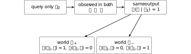
The transcript laws are identical, so Theorem 4.4.3.5 applies, while the deterministic readout returns the same output in both worlds. That output is optimal in \(w_+\) and suboptimal in \(w_-\) on \(x_1\). The example does not show that generalization always fails. It shows that a claim about unqueried utility requires an assumption connecting observed feedback to that utility.
Remark 4.4.3.10. From finite indistinguishability to preference-data limits [ftip-007X]AGENTDRAFTED
Remark 4.4.3.10. From finite indistinguishability to preference-data limits [ftip-007X]AGENTDRAFTED
[zhao2025limits, Theorems 3.3--3.5] study a more structured post-training model. They give ordinal-preference distortion lower bounds, including a lower bound under Bradley--Terry noise with linear scores, and a positive result using a limited number of cardinal queries. These results depend on the routing model, utility class, and query budget developed in § 4.5.2.
Theorem 4.4.3.5 gives a finite pushforward theorem, while Example 4.4.3.9 gives a counterexample to identification from an incomplete transcript. They are neither proofs nor special cases of the paper's distortion results.
4.4.4. Replay monitors and trajectory compression [ftip-007Y]AGENTDRAFTED
4.4.4. Replay monitors and trajectory compression [ftip-007Y]AGENTDRAFTED
Reusing a rollout and jumping along a predicted checkpoint path save different kinds of work. The first changes how often recorded feedback enters an update. The second replaces some realized training steps by a parameter forecast. This subsection records what their proposed monitors establish and, separately, what remains unmeasured.
Theorem 4.4.4.1. DGG head gradient and shared-weight occurrence sum [ftip-007Z]AGENTDRAFTED
Theorem 4.4.4.1. DGG head gradient and shared-weight occurrence sum [ftip-007Z]AGENTDRAFTED
Fix a sampled history and an active token \(i\) in the interior of the unclipped branch of the GRPO objective. Consider a finite directed acyclic computation graph that is differentiable at the parameter point in question. Let \(a_i\) be the sampled token, \(\widehat A_i\) its fixed normalized advantage, and \(p_i=\operatorname {softmax}(z_i)\) the current distribution on a finite vocabulary \(\mathcal V\). With fixed behavior probability \(b_i>0\), set \[ r_i=\frac {p_i(a_i)}{b_i}, \qquad \mathcal L_i=r_i\widehat A_i, \qquad E_i=r_i\widehat A_i(e_{a_i}-p_i). \] Here \(e_{a_i}\in \mathbb R^{|\mathcal V|}\) is the sampled-token basis vector. The history and sampling decisions are held fixed during differentiation.
Suppose the output head \(W_{\rm lm}\in \mathbb R^{|\mathcal V|\times d_{\rm model}}\) is untied: its only path to \(\mathcal L_i\) is through \(z_i=W_{\rm lm}h_{L,i}\), and \(h_{L,i}\in \mathbb R^{d_{\rm model}}\) is independent of \(W_{\rm lm}\). Then \[ G_i^{\rm lm}=\nabla _{W_{\rm lm}}\mathcal L_i =E_i h_{L,i}^{\mathsf T}. \]
Let \(W_{\rm int}\in \mathbb R^{m\times d}\) be a shared intermediate weight. Index by a finite set \(\mathcal O_i\) every occurrence of this weight that can affect \(z_i\), assuming that all such uses have the form \(y_o=W_{\rm int}x_o\), with \(x_o\in \mathbb R^d\). First replace these uses by independent copies \(W_o\) and evaluate them all at \(W_o=W_{\rm int}\). Let \(J_{io}\in \mathbb R^{|\mathcal V|\times m}\) be the downstream Jacobian from node \(y_o\) to \(z_i\) in this graph, with the other weight copies fixed. Define the contribution of occurrence \(o\) by \[ H_{io}=\nabla _{W_o}\mathcal L_i =(J_{io}^{\mathsf T}E_i)x_o^{\mathsf T}. \] On tying the copies, the total derivative is \[ G_i^{\rm int}=\nabla _{W_{\rm int}}\mathcal L_i =\sum _{o\in \mathcal O_i}H_{io}. \] The head gradient and each occurrence contribution have rank at most one; the total shared-weight gradient need not.
For a layer used once per position in a causal network, the sum includes every earlier position whose output affects token \(i\). Reuse across depth adds further occurrences. Tying the head to embeddings or other blocks also requires their contributions; the displayed head identity assumes that such tying is absent.
Proof.
Proof.
Softmax differentiation gives \(\nabla _{z_i}\mathcal L_i=E_i\). The outer-product rule gives the untied head identity. In the graph with independent copies, \(x_o\) does not depend on its own \(W_o\); all downstream paths from \(y_o\) are included in \(J_{io}\). The chain rule therefore gives \(\nabla _{W_o}\mathcal L_i=(J_{io}^{\mathsf T}E_i)x_o^{\mathsf T}\). Finally, the derivative of the diagonal map \(W_{\rm int}\mapsto (W_o=W_{\rm int})_{o\in \mathcal O_i}\) adds these partial derivatives.
Clipped or inactive terms require their own derivative or mask. [miao2026when, Section 4.2.1, Proposition 1, and Appendix A.1] derives the intermediate outer product through one local application. For a shared weight, that calculation gives \(H_{io}\); identifying it with the total \(G_i^{\rm int}\) omits the other occurrences. The sum above supplies the chain rule needed for shared parameters.
Theorem 4.4.4.2. DGG occurrence-to-head gradient-energy bound [ftip-0080]AGENTDRAFTED
Theorem 4.4.4.2. DGG occurrence-to-head gradient-energy bound [ftip-0080]AGENTDRAFTED
Use the per-token quantities and untied head of Theorem 4.4.4.1, and fix one occurrence \(o\in \mathcal O_i\). Assume \(d_{\rm model}\geq 1\) and positive constants \(\alpha _{\min }\), \(\beta _{\max }\), and \(C\) satisfy \[ \|h_{L,i}\|_2^2\geq \alpha _{\min }d_{\rm model}, \qquad \|x_o\|_2^2\leq \beta _{\max }d_{\rm model}, \] and the two logit-sensitivity bounds \[ \mathbb E_{a\sim p_i} \|(J_{io})_{a,:}\|_2^2\leq C, \qquad \|(J_{io})_{a_i,:}\|_2^2\leq C. \] If \(\widehat A_i\neq 0\) and \(p_i(a_i)<1\), then \[ \frac {\|H_{io}\|_F^2}{\|G_i^{\rm lm}\|_F^2} \leq \frac {\mathcal C_{\rm occ}} {(1-p_i(a_i))^2}, \qquad \mathcal C_{\rm occ} =\frac {4\beta _{\max }C}{\alpha _{\min }}. \]
Proof.
Proof.
The sampled-token coordinate of \(E_i\) and the lower activation bound give \[ \|G_i^{\rm lm}\|_F^2 =\|E_i\|_2^2\|h_{L,i}\|_2^2 \geq r_i^2\widehat A_i^2 (1-p_i(a_i))^2 \alpha _{\min }d_{\rm model}. \] Write \(J_{io}^{\mathsf T}E_i\) as \(r_i\widehat A_i\) times the difference between the sampled row and the \(p_i\)-weighted mean row. The squared-norm inequality \(\|u-v\|_2^2\leq 2\|u\|_2^2+2\|v\|_2^2\), Jensen's inequality for that mean, and the two row-energy bounds give \(\|J_{io}^{\mathsf T}E_i\|_2^2\leq 4r_i^2\widehat A_i^2C\). Hence \[ \|H_{io}\|_F^2 \leq 4r_i^2\widehat A_i^2C\, \beta _{\max }d_{\rm model}. \] The source's softmax probabilities make \(r_i>0\); the nonzero-advantage and nonunit-probability hypotheses make the head lower bound positive. Division and cancellation give the displayed ratio.
This bounds one occurrence contribution, not the total derivative of a shared intermediate weight. For the latter, the sum in Theorem 4.4.4.1 gives only \[ \|G_i^{\rm int}\|_F \leq \sum _{o\in \mathcal O_i} \|J_{io}^{\mathsf T}E_i\|_2\|x_o\|_2. \] If the same displayed hypotheses hold for every occurrence, the triangle inequality yields the ratio bound \(|\mathcal O_i|^2\mathcal C_{\rm occ}/(1-p_i(a_i))^2\) for \(\|G_i^{\rm int}\|_F^2/\|G_i^{\rm lm}\|_F^2\). Controlling only the application at position \(i\) does not establish this all-occurrence hypothesis or the source's claimed bound for the total gradient. The contributing positions, reuse pattern, and Jacobians depend on the architecture. Neither bound establishes a small gradient or an evaluation-score comparison.
The activation and row-energy hypotheses and the local inequality follow the calculation in [miao2026when, Section 4.2.1, Lemma 1, Assumption 1, Theorem 1, and Appendix A.3], with the differentiated object restricted to an occurrence contribution. They do not prove the source's total shared-weight claim under its local hypotheses.
Theorem 4.4.4.3. DGG finite-batch head-gradient inequality [ftip-0081]AGENTDRAFTED
Theorem 4.4.4.3. DGG finite-batch head-gradient inequality [ftip-0081]AGENTDRAFTED
For \(T\geq 1\) active, unclipped tokens with fixed sampled histories and the untied output head of Theorem 4.4.4.1, let \[ G^{\rm lm}=\frac 1T\sum _{i=1}^T G_i^{\rm lm}, \qquad \overline {r^2}=\frac 1T\sum _{i=1}^T r_i^2, \] and set \[ c_{\max }= \max _{1\leq i\leq T} \widehat A_i^2 \|e_{a_i}-\pi _\theta (\mathord \cdot \mid h_{L,i})\|_2^2 \|h_{L,i}\|_2^2. \] Then \[ \|G^{\rm lm}\|_F^2\leq c_{\max }\overline {r^2} =c_{\max }(1+\widehat \chi ^2), \] where \(\widehat \chi ^2\) is the statistic of Definition 4.3.13. If \(c_{\max }>0\), rearrangement gives the source's equivalent direction \[ \widehat \chi ^2\geq \frac {\|G^{\rm lm}\|_F^2}{c_{\max }}-1. \]
Proof.
Proof.
Convexity of the squared Frobenius norm and the factorization in Theorem 4.4.4.1 give \[ \left \|\frac 1T\sum _iG_i^{\rm lm}\right \|_F^2 \leq \frac 1T\sum _i\|G_i^{\rm lm}\|_F^2 \leq \frac {c_{\max }}T\sum _i r_i^2. \] The identity \(\overline {r^2}=1+\widehat \chi ^2\) follows directly from Definition 4.3.13; division by positive \(c_{\max }\) gives the final form.
The inequality points from observed head-gradient energy to a lower bound on this finite-batch squared-ratio statistic. It is not a converse: cancellation can hide nonunit ratios. The active cancellation example in Example 4.4.4.6 states its clipping interval explicitly. The proof uses no intermediate-weight bound.
The finite-batch inequality follows the calculation in [miao2026when, Section 4.2.2, Lemma 2, Theorem 2, and Appendix B], under the untied-head and fixed-history assumptions stated above.
Remark 4.4.4.4. DGG monitors update geometry, not evaluation safety [ftip-0082]AGENTDRAFTED
Remark 4.4.4.4. DGG monitors update geometry, not evaluation safety [ftip-0082]AGENTDRAFTED
The identities in Theorem 4.4.4.1--Theorem 4.4.4.3 concern gradients, importance ratios, activations, and occurrence-specific logit Jacobians. The intermediate bound controls a local contribution; a shared-weight bound needs control over all contributing occurrences. None of their hypotheses mentions the fixed independent-evaluation functional \(J_{\rm ev}\) of Definition 4.1.2. They therefore cannot imply that accepting an update preserves \(J_{\rm ev}\), or that rejecting one would have prevented a decrease.
DGG adds an empirical policy on top of those identities: it monitors the increment in head-gradient energy, standardizes that increment against a trailing window, and rejects some reused updates before the optimizer step [miao2026when, Section 5 and Algorithm 1]. Its reported experiments relate that policy to observed training stability. They do not turn the Z-score into a calibrated test of independent-evaluation safety.
Example 4.4.4.5. Counterexample: empirical squared-ratio excess can be negative [ftip-0083]AGENTDRAFTED
Example 4.4.4.5. Counterexample: empirical squared-ratio excess can be negative [ftip-0083]AGENTDRAFTED
Take one observed action \(a\) with \(\pi _{\rm old}(a)=1/2\) and \(\pi _\theta (a)=1/4\). The batch contains only that action, so \(T=1\) and \(r_1=1/2\). Hence \[ \widehat \chi ^2=r_1^2-1=-\frac 34. \] Both policies can be completed on a two-action space by assigning their remaining mass to the other action.
Thus the finite-batch statistic in Definition 4.3.13 need not share the nonnegativity of the population Pearson divergence. Theorem Theorem 4.4.4.3 remains valid: its right side contains \(1+\widehat \chi ^2=1/4=\overline {r^2}\).
Example 4.4.4.6. Counterexample: active batch cancellation can hide nonunit ratios [ftip-0084]AGENTDRAFTED
Example 4.4.4.6. Counterexample: active batch cancellation can hide nonunit ratios [ftip-0084]AGENTDRAFTED
Fix \(\epsilon _{\rm clip}\in (0,1)\) and \(1<R<1+\epsilon _{\rm clip}\). On a two-token vocabulary, let both observed tokens have \(a_i=1\), current probability \(\pi _\theta (1)=1/2\), and behavior probability \(\pi _{\rm old}(1)=1/(2R)\). Take scalar hidden states \(h_{L,1}=h_{L,2}=1\) and fixed normalized advantages \(\widehat A_1=1\), \(\widehat A_2=-1\). These may be selected token terms from different rollout members. An untied head with both logits zero realizes the current probabilities. Both terms lie strictly inside the clipping interval of Definition 2.6.8, so the clipped surrogate locally agrees with \(\mathcal L_i=r_i\widehat A_i\). Thus \(r_1=r_2=R\), and Theorem 4.4.4.1 gives \[ G_1^{\rm lm}=R(1/2,-1/2)^{\mathsf T}, \qquad G_2^{\rm lm}=-G_1^{\rm lm}. \] Consequently \(G^{\rm lm}=0\), while \(\widehat \chi ^2=R^2-1>0\). For this fixed clipping rule, the statistic in this construction is bounded above by \((1+\epsilon _{\rm clip})^2-1\).
For the raw surrogate \(\mathcal L_i=r_i\widehat A_i\) considered as a separate objective, the same algebra works at every \(R>1\) and yields arbitrarily large squared-ratio excess. This does not extend the active construction to arbitrary \(R\) under clipping: when \(R>1+\epsilon _{\rm clip}\), the positive-advantage term is locally constant, while the negative term remains active. Their clipped gradients are then \(0\) and \(-R(1/2,-1/2)^{\mathsf T}\), with nonzero mean \((-R/4,R/4)^{\mathsf T}\).
The example does not contradict Theorem 4.4.4.3: that theorem upper-bounds batch-gradient energy by a ratio moment. It supplies no lower bound on the gradient and no converse from zero batch-gradient energy to ratios equal to one. The arbitrary-ratio version concerns only the separate raw surrogate.
Example 4.4.4.7. Counterexample: a Z-score gate is not an evaluation-safety certificate [ftip-0085]AGENTDRAFTED
Example 4.4.4.7. Counterexample: a Z-score gate is not an evaluation-safety certificate [ftip-0085]AGENTDRAFTED
Let two consecutive proposed reused updates have the same monitored energy, \(g_{t-1}=g_t=1\). With trailing-window increment mean \(\mu _t=0\), any positive scale \(\sigma _t+\varepsilon \), and any positive threshold, DGG's score is \[ z_t=\frac {(g_t-g_{t-1})-\mu _t}{\sigma _t+\varepsilon }=0, \] so the gate accepts the proposal. Now choose a fixed evaluation interface for which the artifact before the accepted update has performance \(J_{\rm ev}=1\) and the artifact after it has performance \(J_{\rm ev}=0\).
This is consistent because the gate rule of Definition 2.11.13 imposes no mathematical relation between its scalar monitor and \(J_{\rm ev}\). A safety claim would need an additional assumption connecting proposed updates to the independent evaluation law; the Z-score calculation alone cannot provide it.
Definition 4.4.4.8. Leading squared singular-energy share [ftip-0086]AGENTDRAFTED
Definition 4.4.4.8. Leading squared singular-energy share [ftip-0086]AGENTDRAFTED
Let \(\Delta W\in \mathbb R^{m\times n}\) be nonzero, set \(q=\min (m,n)\), and order its singular values as \(\sigma _1\geq \cdots \geq \sigma _q\geq 0\). Its leading squared singular-energy share is \[ \rho _1(\Delta W) =\frac {\sigma _1(\Delta W)^2}{\sum _{j=1}^q\sigma _j(\Delta W)^2} =\frac {\sigma _1(\Delta W)^2}{\|\Delta W\|_F^2}. \] The nonzero hypothesis prevents an undefined \(0/0\); the value lies in \([1/q,1]\).
NExt instead reports \(E_1=\sigma _1/\sum _j\sigma _j\) in Section 3.2 Low-rank optimization trajectories modeling for LLM RLVR acceleration[chen2026lowrank]. That nuclear-share statistic and \(\rho _1\) answer different questions. The squared share measures contribution to squared Frobenius norm.
Definition 4.4.4.9. Leading spectral gap [ftip-0087]AGENTDRAFTED
Definition 4.4.4.9. Leading spectral gap [ftip-0087]AGENTDRAFTED
For \(\Delta W\in \mathbb R^{m\times n}\) with \(q=\min (m,n)\geq 2\), its leading spectral gap is \[ \operatorname {gap}_1(\Delta W) =\sigma _1(\Delta W)-\sigma _2(\Delta W). \] A positive gap makes the leading left and right one-dimensional singular subspaces unique, although each chosen singular vector still has an arbitrary sign. When the gap is zero, a single leading vector is not intrinsic.
The quantity is undefined when \(q=1\), since there is no second singular value. Projector comparisons require a positive gap at every compared checkpoint.
Definition 4.4.4.10. Leading-subspace projector drift [ftip-0088]AGENTDRAFTED
Definition 4.4.4.10. Leading-subspace projector drift [ftip-0088]AGENTDRAFTED
Let \(\Delta W_t\) and \(\Delta W_s\) be nonzero matrices of the same shape, each with positive leading spectral gap. If \(u_1(t)\) and \(u_1(s)\) are unit leading left singular vectors, define their leading-subspace projector drift by \[ d_{\rm proj}(t,s) =\|\Pi _t^{\rm svd}-\Pi _s^{\rm svd}\|_F, \qquad \Pi _t^{\rm svd}=u_1(t)u_1(t)^{\mathsf T}, \quad \Pi _s^{\rm svd}=u_1(s)u_1(s)^{\mathsf T}. \] The definition is independent of both singular-vector signs and takes values in \([0,\sqrt {2}]\).
This is an additional proposed trajectory diagnostic; NExt does not define it.
A large value of \(\rho _1\) from Definition 4.4.4.8 says that one singular mode dominates a particular difference matrix. It does not say that the dominant subspace remains fixed across checkpoints; \(d_{\rm proj}\) measures that separate question.
Definition 4.4.4.11. Path-emulation regret [ftip-0089]AGENTDRAFTED
Definition 4.4.4.11. Path-emulation regret [ftip-0089]AGENTDRAFTED
Fix the evaluation interface of Convention 4.1.1. Let \(P_{t+s}^{\rm act}\) be the protocol that returns the artifact reached after \(s\geq 1\) additional realized training steps from checkpoint \(t\). Let \(\mathcal K_{\leq t}\) be the saved checkpoint history available through \(t\), and let \(\widehat P_{t+s}(\mathcal K_{\leq t})\) instead return the artifact forecast from that history. Their signed path-emulation regret and absolute path-emulation regret are \[ \begin {aligned} \operatorname {Reg}^{\rm path}_{\rm ev}(t,s) &=J_{\rm ev}(P_{t+s}^{\rm act}) -J_{\rm ev}(\widehat P_{t+s}(\mathcal K_{\leq t})),\\ \operatorname {AReg}^{\rm path}_{\rm ev}(t,s) &=\left |\operatorname {Reg}^{\rm path}_{\rm ev}(t,s)\right |. \end {aligned} \]
The sign distinguishes an optimistic forecast from a pessimistic one; the absolute value measures discrepancy without cancellation across checkpoints. Both use the same task law, inference budget, and evaluator. Parameter error alone is not substituted for evaluation error. The NExt extrapolation and recovery schedule described in Sections 4.1--4.3 and 5.1 motivates this comparison Low-rank optimization trajectories modeling for LLM RLVR acceleration[chen2026lowrank], but the paper does not state this regret definition.
Example 4.4.4.12. Counterexample: early low-rank agreement does not determine continuation [ftip-008A]AGENTDRAFTED
Example 4.4.4.12. Counterexample: early low-rank agreement does not determine continuation [ftip-008A]AGENTDRAFTED
Let \(e_1=(1,0)^{\mathsf T}\) and \(e_2=(0,1)^{\mathsf T}\) be the standard basis vectors of \(\mathbb R^2\). In a two-dimensional matrix chart, set \(P=e_1e_1^{\mathsf T}\) and \(Q=e_2e_2^{\mathsf T}\). Two paths share the entire observed history \[ W_0=0,\qquad W_1=P,\qquad W_2=2P. \] Every observed local difference is the same rank-one matrix \(P\). The paths then fork: path A takes \(W_3^A=3P\), whereas path B takes \(W_3^B=2P+Q\). Each next local difference is again rank one.
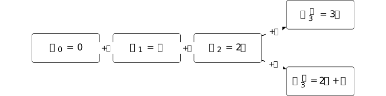
A deterministic history-only forecaster must return the same matrix \(\widehat W_3\) in both worlds. Since \(\|W_3^A-W_3^B\|_F=\|P-Q\|_F=\sqrt {2}\), the triangle inequality forces its Frobenius error to be at least \(1/\sqrt {2}\) on one continuation. Low-rank early motion therefore does not identify the next subspace or the next checkpoint.
Remark 4.4.4.13. Compression of a charted path is not capability acquisition [ftip-008B]AGENTDRAFTED
Remark 4.4.4.13. Compression of a charted path is not capability acquisition [ftip-008B]AGENTDRAFTED
NExt extracts global, local, and target differences from LoRA checkpoint matrices, keeps leading singular factors, learns a nonlinear predictor, jumps in that parameter chart, and resumes RLVR [chen2026lowrank, Sections 3.2, 4.1--4.3, and 5.1]. Its reported results are empirical; the paper states no theorem that a leading subspace remains stable or that a forecast preserves a policy.
The quantities in Definition 4.4.4.8--Definition 4.4.4.11 separate four tests. Squared singular-energy share concerns one matrix, spectral gap controls whether its leading subspace is identifiable, projector drift compares those subspaces over time, and path-emulation regret returns to fixed independent evaluation. None, by itself, is evidence that new feedback was acquired or that a new capability was learned. Such a claim must use a declared post-training gain such as Definition 4.1.3 and must charge forecast training, the parameter jump, and recovery updates.
4.5. Alignment gain and preference information [ftip-008E]AGENTDRAFTED
4.5. Alignment gain and preference information [ftip-008E]AGENTDRAFTED
Two finite models ask different questions about post-training. The first assumes an exact KL-regularized optimizer and characterizes the reward gain that its exponential tilt can produce. The second asks what ordinal comparisons reveal when post-training may reroute a fixed set of response circuits.
Neither source model is a general account of neural post-training. The first assumes exact optimization of a declared scalar reward. The second is a stylized routing model with a fixed circuit set. Extending the KL identity to an approximate optimizer requires further analysis. Extending the ordinal routing conclusion to a changing circuit set requires additional assumptions on that change.
4.5.1. Finite KL-regularized alignment [ftip-008F]AGENTDRAFTED
4.5.1. Finite KL-regularized alignment [ftip-008F]AGENTDRAFTED
This subsection studies an exact, finite optimization model. A reference law is exponentially tilted by a declared scalar reward. In this setting, reward gain admits two exact descriptions: a Jeffreys-divergence identity and a covariance under the reference law.
The statements do not model approximate optimization, neural training cost, reward validity, or independent capability evaluation.
Remark 4.5.1.1. Exact optimization on a finite response set [ftip-008G]AGENTDRAFTED
Remark 4.5.1.1. Exact optimization on a finite response set [ftip-008G]AGENTDRAFTED
Theorems 1 and 2 of the v1 preprint [paes2026theoretical] concern an exactly optimal KL-regularized policy and a fixed query. On a finite response set, their expectations and normalizers are ordinary finite sums.
These exact identities do not establish a comparison among best-of-\(N\), PPO, and GRPO, or a general guarantee for proxy rewards and reward ensembles. Those questions require assumptions beyond exact optimization of one reward.
Notation 4.5.1.2. Translating the alignment source notation [ftip-008H]AGENTDRAFTED
Notation 4.5.1.2. Translating the alignment source notation [ftip-008H]AGENTDRAFTED
The source writes \(\lambda >0\) for the KL penalty. Here we write \(\beta >0\), matching the DPO notation in Notation 2.7.1--Definition 2.7.3. This avoids collision with the generalized-advantage parameter in Definition 2.6.7 and the protocol law in Definition 4.4.3.1.
The source's gain \(\Delta (r,r')\) is written \(G_p(r;s)\): \(r\) is the reward used to tilt the reference law \(p\), while \(s\) is the reward used to evaluate the tilted law. This avoids collision with both the simplex notation \(\Delta (X)\) of Notation 1.2.1 and the paired DPO margin of Notation 2.7.1. For a finite set \(\mathcal Y\), a law \(p\in \Delta (\mathcal Y)\), and functions \(f,g:\mathcal Y\to \mathbb R\), set
\[ \operatorname {Cov}_p(f,g) =\mathbb E_{y\sim p}[f(y)g(y)] -\mathbb E_{y\sim p}[f(y)]\, \mathbb E_{y\sim p}[g(y)]. \]
Definition 4.5.1.3. Finite KL-alignment instance [ftip-008I]AGENTDRAFTED
Definition 4.5.1.3. Finite KL-alignment instance [ftip-008I]AGENTDRAFTED
A finite KL-alignment instance consists of a nonempty finite response set \(\mathcal Y\), a reference law \(p\in \Delta (\mathcal Y)\), a penalty \(\beta >0\), and finite real functions \(r,s:\mathcal Y\to \mathbb R\). The reference support is
\[ S_p=\{y\in \mathcal Y:p(y)>0\}. \]A prompt is fixed and suppressed. The function \(r\) determines the alignment update; \(s\) measures its result. They may coincide, but they need not. Finiteness makes every exponential weight and expectation below finite.
These objects specialize the fixed-query setting in [paes2026theoretical, Section 2, equations (2.1)--(2.2)]; they are not a definition of alignment in general.
Definition 4.5.1.4. Exponential weight and partition function [ftip-008J]AGENTDRAFTED
Definition 4.5.1.4. Exponential weight and partition function [ftip-008J]AGENTDRAFTED
For a finite KL-alignment instance, define the exponential weight and partition function by
\[ a_r(y)=\exp \left (\frac {r(y)}{\beta }\right ), \qquad Z_r=\mathbb E_{y\sim p}[a_r(y)]. \]Every \(a_r(y)\) is finite and strictly positive. Since \(p\) is a probability law on a nonempty finite set, \(0<Z_r<\infty \).
This weight and normalizer are the fixed-query form of [paes2026theoretical, Equation (2.2)].
Definition 4.5.1.5. Aligned law in finite-source notation [ftip-008K]AGENTDRAFTED
Definition 4.5.1.5. Aligned law in finite-source notation [ftip-008K]AGENTDRAFTED
The aligned law induced by \(r\) is \(q_r\in \Delta (\mathcal Y)\) given by
\[ q_r(y)=\frac {p(y)a_r(y)}{Z_r}. \]Normalization follows from the definition of \(Z_r\). Moreover, \(q_r(y)>0\) exactly when \(p(y)>0\). This is the finite notation for the same exponential-tilt optimizer stated in Definition 2.7.3; support preservation was proved in Theorem 4.4.1.6.
This formula is [paes2026theoretical, Equation (2.2)]. It assumes the exact optimizer, not an iterate returned by a particular training algorithm.
Definition 4.5.1.6. Cross-reward gain under an alignment reward [ftip-008L]AGENTDRAFTED
Definition 4.5.1.6. Cross-reward gain under an alignment reward [ftip-008L]AGENTDRAFTED
The cross-reward gain from aligning with \(r\) and evaluating with \(s\) is
\[ G_p(r;s) =\mathbb E_{y\sim q_r}[s(y)] -\mathbb E_{y\sim p}[s(y)]. \]The semicolon records two roles. Its left argument changes the response law; its right argument scores both laws. Thus \(G_p(r;s)\) is not an independent evaluation unless \(s\) has separately been declared to serve that role.
This is the finite notation for \(\Delta (r,r')\) in Theorem 2, equation (3.4), of Theoretical limits of language model alignment[paes2026theoretical].
Definition 4.5.1.7. Jeffreys divergence [ftip-008M]AGENTDRAFTED
Definition 4.5.1.7. Jeffreys divergence [ftip-008M]AGENTDRAFTED
For probability laws \(p\) and \(q\) for which both terms are finite, their Jeffreys divergence is
\[ J(p,q) =D_{\mathrm {KL}}(p\Vert q) +D_{\mathrm {KL}}(q\Vert p). \]The KL divergence and its argument order are defined in Definition 2.6.3. Unlike either directed term, \(J(p,q)=J(q,p)\). In the finite tilt of Definition 4.5.1.5, \(p\) and \(q_r\) have the same support, so both terms are finite.
Lemma 4.5.1.8. Log-density ratio of the exact tilt [ftip-008N]AGENTDRAFTED
Lemma 4.5.1.8. Log-density ratio of the exact tilt [ftip-008N]AGENTDRAFTED
For every \(y\in S_p\), the aligned law satisfies
\[ \log \frac {q_r(y)}{p(y)} =\frac {r(y)}{\beta }-\log Z_r. \]
Proof.
Proof.
On \(S_p\), both \(p(y)\) and \(q_r(y)\) are positive. Dividing the formula of Definition 4.5.1.5 by \(p(y)\) and taking logarithms gives the identity.
This is equation (B.1) followed by the logarithmic step in [paes2026theoretical, Appendix B.1, equations (B.1)--(B.2)].
Theorem 4.5.1.9. Exact reward gain equals scaled Jeffreys divergence [ftip-008O]AGENTDRAFTED
Theorem 4.5.1.9. Exact reward gain equals scaled Jeffreys divergence [ftip-008O]AGENTDRAFTED
For a finite KL-alignment instance,
\[ G_p(r;r)=\beta J(p,q_r). \]
Proof.
Proof.
Rearranging Lemma 4.5.1.8 gives \(r(y)=\beta \log (q_r(y)/p(y))+\beta \log Z_r\) on the common support. Taking expectation first under \(q_r\) and then under \(p\) yields
\[ \begin {aligned} \mathbb E_{q_r}[r] &=\beta D_{\mathrm {KL}}(q_r\Vert p)+\beta \log Z_r,\\ \mathbb E_p[r] &=-\beta D_{\mathrm {KL}}(p\Vert q_r)+\beta \log Z_r. \end {aligned} \]Subtracting cancels the common normalizer and gives the result.
This is the finite form of [paes2026theoretical, Theorem 1, equation (3.2), with proof in Appendix B.1].
Remark 4.5.1.10. What the Jeffreys identity does and does not identify [ftip-008P]AGENTDRAFTED
Remark 4.5.1.10. What the Jeffreys identity does and does not identify [ftip-008P]AGENTDRAFTED
The identity Theorem 4.5.1.9 is an equality inside one declared model. It says that exact gain in the optimizing reward equals a symmetric divergence from the reference law. It does not say that a larger divergence improves a different utility, nor that a training algorithm reaches the exact tilt.
The identity accounts for neither rollout and update work nor the cost of obtaining \(r\). Consequently it is not, by itself, a bound on the costed post-training potential of Definition 4.1.10.
Theorem 4.5.1.11. Cross-reward gain is a base-law covariance [ftip-008Q]AGENTDRAFTED
Theorem 4.5.1.11. Cross-reward gain is a base-law covariance [ftip-008Q]AGENTDRAFTED
For a finite KL-alignment instance,
\[ G_p(r;s) =\operatorname {Cov}_p\left (s,\frac {a_r}{Z_r}\right ). \]
Proof.
Proof.
The aligned expectation can be written under the reference law as \(\mathbb E_{q_r}[s]=\mathbb E_p[s a_r/Z_r]\). Also \(\mathbb E_p[a_r/Z_r]=1\). Substituting these two identities into Definition 4.5.1.6 gives the covariance defined in Notation 4.5.1.2.
This is the finite form of Theorem 2, equation (3.4), in Theoretical limits of language model alignment[paes2026theoretical]. Its proof is in Appendix B.1, equations (B.5)--(B.7).
Remark 4.5.1.12. The covariance is predictive only for a declared reward [ftip-008R]AGENTDRAFTED
Remark 4.5.1.12. The covariance is predictive only for a declared reward [ftip-008R]AGENTDRAFTED
The identity Theorem 4.5.1.11 expresses exact tilted-law gain using expectations under \(p\). This makes the population quantity accessible from the reference law in principle. A finite-sample estimator still needs its own sampling law, moment assumptions, and error analysis.
The formula also remains indexed by both \(r\) and \(s\). It cannot turn a proxy reward into an independent utility. If \(s=r\), it measures improvement in the same quantity that defined the exact optimizer; if \(s\ne r\), its sign is determined by the displayed covariance.
Example 4.5.1.13. A two-response alignment identity [ftip-008S]AGENTDRAFTED
Example 4.5.1.13. A two-response alignment identity [ftip-008S]AGENTDRAFTED
Take \(\mathcal Y=\{a,b\}\), \(p=(1/2,1/2)\), \(\beta =1\), and \(r(a)=0\), \(r(b)=\log 3\). Exponential weighting changes the reference law as follows.

The reward gain is
\[ G_p(r;r) =\left (\frac 34-\frac 12\right )\log 3 =\frac 14\log 3. \]Direct calculation gives
\[ \begin {aligned} D_{\mathrm {KL}}(q_r\Vert p) &=\frac 14\log \frac 12+\frac 34\log \frac 32,\\ D_{\mathrm {KL}}(p\Vert q_r) &=\frac 12\log 2+\frac 12\log \frac 23, \end {aligned} \]whose sum is \(\frac 14\log 3\). Thus the example checks Theorem 4.5.1.9 exactly; it is not an empirical alignment result.
Corollary 4.5.1.14. Averaging the fixed-query identity over prompts [ftip-008T]AGENTDRAFTED
Corollary 4.5.1.14. Averaging the fixed-query identity over prompts [ftip-008T]AGENTDRAFTED
Let \(\mathcal X\) be finite with prompt law \(\mu \). For each \(x\in \mathcal X\), let \(p_x\), \(r_x\), and \(q_{r_x}\) be a finite KL-alignment instance with the same penalty \(\beta >0\). Then
\[ \sum _{x\in \mathcal X}\mu (x)G_{p_x}(r_x;r_x) =\beta \sum _{x\in \mathcal X}\mu (x)J(p_x,q_{r_x}). \]
Proof.
Proof.
Apply Theorem 4.5.1.9 at each prompt and take the finite \(\mu \)-weighted sum.
The source theorem is stated for each fixed query. This corollary performs only finite averaging; it does not introduce a shared neural parameterization across prompts.
Lemma 4.5.1.15. Additive reward shifts leave the aligned law unchanged [ftip-008U]AGENTDRAFTED
Lemma 4.5.1.15. Additive reward shifts leave the aligned law unchanged [ftip-008U]AGENTDRAFTED
For constants \(c,d\in \mathbb R\),
\[ q_{r+c}=q_r, \qquad G_p(r+c;s+d)=G_p(r;s). \]
Proof.
Proof.
The shifted weight is \(a_{r+c}=e^{c/\beta }a_r\), while its partition function is \(Z_{r+c}=e^{c/\beta }Z_r\); the common factor cancels in the aligned law. Adding \(d\) to the evaluation reward adds \(d\) to both expectations in the gain, so it also cancels.
This finite lemma records the same prompt-dependent additive non-identifiability that appears in the DPO reparameterization of Definition 2.7.4.
Remark 4.5.1.16. A penalty coefficient is not a hard KL budget [ftip-008V]AGENTDRAFTED
Remark 4.5.1.16. A penalty coefficient is not a hard KL budget [ftip-008V]AGENTDRAFTED
For fixed \(\beta \), the exponential tilt solves the penalized problem
\[ \max _{q\in \Delta (\mathcal Y)} \left \{\mathbb E_q[r] -\beta D_{\mathrm {KL}}(q\Vert p)\right \} \]under the conventions of Definition 4.5.1.3. This is not the same specification as choosing a number \(\kappa \) and solving
\[ \max _q\mathbb E_q[r] \quad \text {subject to}\quad D_{\mathrm {KL}}(q\Vert p)\leq \kappa . \]A Lagrange multiplier can relate the two problems when the relevant duality and activity conditions hold. The coefficient \(\beta \) alone does not declare a hard budget, and the identities Theorem 4.5.1.9--Theorem 4.5.1.11 do not supply those conditions.
Remark 4.5.1.17. Fixed-query identities and their assumptions [ftip-008W]AGENTDRAFTED
Remark 4.5.1.17. Fixed-query identities and their assumptions [ftip-008W]AGENTDRAFTED
The source setup writes rewards as \(r(\mathbf x,\mathbf y)\), while the display of Theorem 1 reverses the two arguments in places. This subsection uses the setup order and then suppresses the fixed prompt. The source also moves between a dataset-level penalized objective and fixed-query identities. The finite-averaging result Corollary 4.5.1.14 makes that step explicit.
The identities specialize Theoretical limits of language model alignment[paes2026theoretical] to a finite response set. They require no extension to the full sequence space.
Finally, exact exponential tilting is a distributional optimizer. It does not account for rollout, gradient, optimizer, or systems cost, and it does not show that PPO, GRPO, DPO, or any frontier training run attains the displayed law. Applying the identities to a training run therefore requires a separate argument that its output law is the exact optimizer.
4.5.2. Preference-feedback distortion [ftip-008X]AGENTDRAFTED
4.5.2. Preference-feedback distortion [ftip-008X]AGENTDRAFTED
A finite routing model supports preference-distortion lower bounds in Sections 2--3 and Appendix A of The limits of preference data for post-training[zhao2025limits]. Cardinal queries permit a different guarantee under the hypotheses of Peeking behind the ordinal curtain: Improving distortion via cardinal queries[amanatidis2021peeking].
Both comparisons depend on the queries, circuits, routing maps, utility, feedback profile, algorithm, and comparator class. The noiseless and Bradley--Terry bounds retain those model restrictions.
Remark 4.5.2.1. The routing-model assumption behind preference limits [ftip-008Y]AGENTDRAFTED
Remark 4.5.2.1. The routing-model assumption behind preference limits [ftip-008Y]AGENTDRAFTED
The routing model and preference limits below are based on the v1 preprint The limits of preference data for post-training[zhao2025limits]. It models a pretrained system as a finite collection of response circuits plus learned maps that route queries to those circuits. Post-training changes the routing maps while retaining the circuit collection.
The noiseless lower bound is proved here under explicit pointwise response separation and a deterministic preference-only learner, whose returned router may be stochastic. Its finite partition estimate and cardinal-utility construction give a restricted reconstruction of the source rate; the proof does not establish a randomized-learner extension.
The routing model is a source assumption, not an architectural theorem about language models. In particular, its lower bounds do not prove that real post-training creates no circuits, that a neural network decomposes into the displayed objects, or that every preference-learning algorithm obeys the same bound outside this model.
Notation 4.5.2.2. Notation for the finite preference model [ftip-008Z]AGENTDRAFTED
Notation 4.5.2.2. Notation for the finite preference model [ftip-008Z]AGENTDRAFTED
The finite preference model uses the following symbols, corresponding to the notation of The limits of preference data for post-training[zhao2025limits]:
\[ \mathcal Q\mapsto Q,\qquad \mathcal R\mapsto Y,\qquad \mathcal S_0\mapsto C_0,\qquad \mathcal Z\mapsto H, \]\[ \Phi \mapsto \mathfrak E,\qquad \mathcal D\mapsto \mu _Q,\qquad M\mapsto \mathfrak m. \]Thus \(H\) denotes the source's finite internal-representation set, not a public interaction history. The family \(\mathfrak E\) contains admissible query encoders and is unrelated to the costed potential \(\Phi \) of Definition 4.1.10.
Definition 4.5.2.3. Queries, responses, and retained circuits [ftip-0090]AGENTDRAFTED
Definition 4.5.2.3. Queries, responses, and retained circuits [ftip-0090]AGENTDRAFTED
Following the formal model in Section 2 of The limits of preference data for post-training[zhao2025limits], let \(Q\) be a finite nonempty query set and \(Y\) a response set. A response circuit is a function \(c:Q\to Y\). The finite nonempty set \(C_0\) contains the circuits retained from the pretrained model.
The word ``circuit'' is source terminology for this abstract function. No claim is made here that an element of \(C_0\) is localized in a neural network or corresponds to one human-named capability.
Definition 4.5.2.4. Query representation and circuit routing [ftip-0091]AGENTDRAFTED
Definition 4.5.2.4. Query representation and circuit routing [ftip-0091]AGENTDRAFTED
Let \(H\) be a finite nonempty representation set and \(\mathfrak E\subseteq H^Q\) a finite nonempty family of admissible encoders. A query encoder is \(e\in \mathfrak E\). A circuit router is a map
\[ h:H\longrightarrow \Delta (C_0). \]For a query \(\xi \in Q\), the composition \(h(e(\xi ))\) is a law on the retained circuits. Sampling \(c\sim h(e(\xi ))\) and returning \(c(\xi )\) gives the response law. These are the two routing components in the source model [zhao2025limits, Section 2, ``Formal model''].
Definition 4.5.2.5. Pretrained and post-trained routing models [ftip-0092]AGENTDRAFTED
Definition 4.5.2.5. Pretrained and post-trained routing models [ftip-0092]AGENTDRAFTED
A routing model is a triple \(\mathfrak m=(e,h,C_0)\) with the types fixed in Definition 4.5.2.3--Definition 4.5.2.4. The pretrained model is \(\mathfrak m_0=(e_0,h_0,C_0)\). In the source intervention, a post-trained model may replace \(e_0\) and \(h_0\), but it retains exactly \(C_0\).
Write \(\mathfrak m(\xi )\) for the random response obtained by sampling \(c\sim h(e(\xi ))\) and returning \(c(\xi )\). The source sometimes writes this as though the router selected a circuit rather than a distribution; the stochastic reading follows its declared codomain \(\Delta (C_0)\).
Definition 4.5.2.6. Utility and the uniform query law [ftip-0093]AGENTDRAFTED
Definition 4.5.2.6. Utility and the uniform query law [ftip-0093]AGENTDRAFTED
The source fixes the uniform probability law \(\mu _Q\) on \(Q\) and a utility function
\[ u:Q\times Y\longrightarrow \mathbb R. \]For a routing model \(\mathfrak m\), its expected utility is
\[ U_u(\mathfrak m) =\mathbb E_{\xi \sim \mu _Q} \mathbb E\left [u\left (\xi ,\mathfrak m(\xi )\right )\mid \xi \right ]. \]This is the outcome objective in [zhao2025limits, Section 2, ``Outcome-based optimization with preference data'']. It is an assumed cardinal utility, not something ordinal comparisons directly reveal.
Definition 4.5.2.7. Complete noiseless ordinal preference profile [ftip-0094]AGENTDRAFTED
Definition 4.5.2.7. Complete noiseless ordinal preference profile [ftip-0094]AGENTDRAFTED
Assume that distinct retained circuits never tie at a query. For each \(\xi \in Q\), utility then induces a strict comparison by
\[ c_i\succ _{\xi ,u}c_j \quad \Longleftrightarrow \quad u\left (\xi ,c_i(\xi )\right ) >u\left (\xi ,c_j(\xi )\right ). \]The complete noiseless ordinal profile is \(\succ _u=(\succ _{\xi ,u})_{\xi \in Q}\). The source gives the learner unlimited, unbiased access to every such comparison [zhao2025limits, Section 2, final paragraph]. Utilities with ties require a separately declared deterministic tie-break; the lower bounds below use the source's tie-free constructions.
Remark 4.5.2.8. Full preference data and an online oracle expose the same source information [ftip-0095]AGENTDRAFTED
Remark 4.5.2.8. Full preference data and an online oracle expose the same source information [ftip-0095]AGENTDRAFTED
Within this finite model, a table containing every comparison in \(\succ _u\) and a noiseless online oracle that answers every possible query expose the same ordinal information. The source deliberately grants this ideal access so that its obstruction is not caused by finite sampling or an offline split [zhao2025limits, Section 2].
This equivalence does not price the number of queries, labeler time, or adaptivity. It therefore cannot be transferred to a finite-feedback protocol without a separate query-complexity statement.
Definition 4.5.2.9. Preference-only post-training algorithm and attainable route class [ftip-0096]AGENTDRAFTED
Definition 4.5.2.9. Preference-only post-training algorithm and attainable route class [ftip-0096]AGENTDRAFTED
A preference-only post-training algorithm \(\mathcal A\) maps the pretrained routing model and the complete profile to
\[ \mathfrak m_{\mathcal A}(u) =\mathcal A(\mathfrak m_0,\succ _u). \]The deterministic comparator class displayed in the source theorems is
\[ \mathcal M_{\rm det}(C_0) =\left \{(e,h,C_0):e\in \mathfrak E, h:H\to C_0\right \}. \]The source's formal model initially permits stochastic routers \(h:H\to \Delta (C_0)\), but its theorem comparator uses deterministic \(h:H\to C_0\). The comparator class is therefore the displayed deterministic class.
Definition 4.5.2.10. Multiplicative post-training distortion [ftip-0097]AGENTDRAFTED
Definition 4.5.2.10. Multiplicative post-training distortion [ftip-0097]AGENTDRAFTED
Let \(\mathcal B\) be any post-training algorithm with output \(\mathfrak m_{\mathcal B}(u)\) under the feedback law induced by \(u\). When the denominator is positive, define its multiplicative post-training distortion by
\[ \operatorname {Dist}_u(\mathcal B;\mathfrak m_0) =\frac { \max _{\mathfrak m^*\in \mathcal M_{\rm det}(C_0)}U_u(\mathfrak m^*) }{ U_u(\mathfrak m_{\mathcal B}(u)) }. \]If the numerator is positive and the denominator is zero, set the ratio to \(+\infty \). The source lower bounds construct bounded nonnegative utilities for which the comparison is well defined [zhao2025limits, Equation (2) and Appendix A]. Distortion measures loss relative to the declared comparator class; it is not an absolute capability score.
Definition 4.5.2.11. Borda count [ftip-0098]AGENTDRAFTED
Definition 4.5.2.11. Borda count [ftip-0098]AGENTDRAFTED
Let \(m=|C_0|\), and suppose each \(\succ _{\xi ,u}\) is a strict total order on \(C_0\). If \(\operatorname {rank}_{\succ _{\xi ,u}}(c)\) places the most preferred circuit at rank one, its Borda score is
\[ B_{\xi }(c)=m-\operatorname {rank}_{\succ _{\xi ,u}}(c). \]The Borda-count choice is any circuit in
\[ \operatorname *{arg\,max}_{c\in C_0} \sum _{\xi \in Q}B_{\xi }(c). \]This is [zhao2025limits, Definition 3.1]. The source cites a prior equivalence between a standard RLHF model and Borda count; the definition here does not assert that every RLHF implementation is a Borda rule.
Example 4.5.2.12. A compromise circuit can maximize utility without winning Borda count [ftip-0099]AGENTDRAFTED
Example 4.5.2.12. A compromise circuit can maximize utility without winning Borda count [ftip-0099]AGENTDRAFTED
Example 3.2 of The limits of preference data for post-training[zhao2025limits] prints only \(a\geq 0\) and \(2a<b\), but those conditions do not force its stated rankings or Borda totals. Sufficient conditions are \(0<a<1/2\) and \(2a<b<1\). Take three queries, three circuits, and a singleton representation set, so every query must use one common circuit. Set
\[ \begin {array}{c|ccc} &c_A&c_B&c_C\\ \hline \xi _1&1&0&1-a\\ \xi _2&1&0&1-a\\ \xi _3&0&1&b \end {array} \]These inequalities give the rankings \(c_A\succ c_C\succ c_B\) for \(\xi _1,\xi _2\) and \(c_B\succ c_C\succ c_A\) for \(\xi _3\). Hence the Borda totals are \((4,2,3)\), so the ordinal rule selects \(c_A\). The utility totals are \((2,1,2-2a+b)\). Since \(2a<b\), circuit \(c_C\) has strictly greater total utility than \(c_A\).
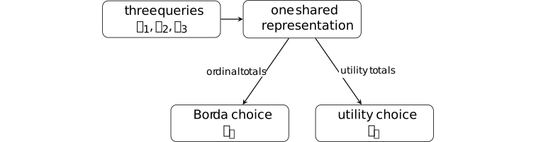
This finite example isolates information lost by ranking. The compromise circuit is never first for an individual query, yet its aggregate utility is largest. It does not show that Borda is always suboptimal or that a neural model must collapse all queries to one representation.
Theorem 4.5.2.13. Noiseless preference distortion for deterministic learners [ftip-009A]AGENTDRAFTED
Theorem 4.5.2.13. Noiseless preference distortion for deterministic learners [ftip-009A]AGENTDRAFTED
Let \(Q,H\) be nonempty finite sets, let \(\varnothing \neq \mathfrak E\subseteq H^Q\) be finite, and let \(C_0=\{c_1,\ldots ,c_m\}\) be a nonempty finite set of deterministic maps \(Q\to Y\). Write \(N=|Q|\), \(r=|H|\), \(p=|\mathfrak E|\) and \(m=|C_0|\). The query law is uniform on \(Q\). Call \(C_0\) pointwise response-separating when
\[ c_i\neq c_j\quad \Longrightarrow \quad c_i(q)\neq c_j(q) \qquad (q\in Q). \]Assume this separation. Let \(\mathcal A\) be a deterministic preference-only learner: from a pretrained model \(\mathfrak m_0\) and the complete strict ordinal profile, it returns \((e,h,C_0)\) with \(e\in \mathfrak E\) and a possibly stochastic router \(h:H\to \Delta (C_0)\). The comparator class is exactly \(\mathcal M_{\rm det}(C_0)\) of Definition 4.5.2.9, including every map \(H\to C_0\) for each \(e\in \mathfrak E\).
For every such pretrained model and learner there exists \(u:Q\times Y\to [0,1]\), inducing a strict profile, such that
\[ \sum _{j=1}^m u(q,c_j(q))=1\quad (q\in Q), \]\[ R_{Q,\mathfrak E,H}=\frac {N}{\sqrt {N(r+\log p)}+r}, \]\[ \operatorname {Dist}_u(\mathcal A;\mathfrak m_0) \geq \frac 1{80}\min \{\sqrt m,R_{Q,\mathfrak E,H}\}. \]Logarithms are natural. Utility averages over the uniform query and the learner's router draw as in Definition 4.5.2.6. The comparator maximum exists because its class is finite and nonempty. It is positive for the normalized utilities above: some constant-circuit route has mean at least \(1/m\). A zero learner utility therefore gives distortion \(+\infty \), with no \(0/0\) case.
Proof.
Proof.
First, for every normalized nonnegative utility, the comparator value is at least the learner value. Keep the learner's representation map and, on each fiber, choose a circuit maximizing its total utility there. That deterministic choice dominates the stochastic mixture and belongs to the comparator class. Thus distortion is at least one.
Put
\[ \begin {aligned} D&=\sqrt {Nr}+\sqrt {\frac N2\log (4p)},& B&=\sqrt {N(r+\log p)},\\ T&=\min \{\sqrt m,R_{Q,\mathfrak E,H}\},& x&=\min \{\sqrt m,N/(2D)\}. \end {aligned} \]Since \((\log 4)/2<1\leq r\) and \(\log p\geq 0\), we have \(D\leq 2B\). Consequently \(N/(2D)\geq N/(4B)\geq R_{Q,\mathfrak E,H}/4\) and \(x\geq T/4\). Every denominator is positive.
If \(m=1\), assign utility one to the sole circuit response at every query. Distortion is one and \(T\leq 1\). If \(m\geq 2\) but \(x<2\), assign the same strict normalized values \(2(m-j)/(m(m-1))\) to the circuits in index order at every query. Distortion is at least one and \(T<8\), which proves the claimed bound. Extend both assignments by zero to all other responses.
In the remaining case set \(k=\lfloor x\rfloor \). Then
\[ 2\leq k\leq \sqrt m,\qquad kD\leq N/2, \qquad k\geq x/2\geq T/8. \]Write \([k]=\{1,\ldots ,k\}\) and fix a map \(f:Q\to [k]\) supplied by Lemma 4.5.2.15. At a query with label \(i=f(q)\), fix the strict order putting \(c_i\) first and the remaining circuits in increasing index order. Let \(\operatorname {rank}_i(j)\in \{1,\ldots ,m\}\) be the position of \(c_j\), with the first circuit at rank one, and define
\[v_i(j)=\frac {2(m-\operatorname {rank}_i(j))}{m(m-1)}.\]These values decrease strictly in the fixed order, sum to one and lie in \([0,2/m]\). The ordinal profile is now fixed independently of the learner's output. Run the deterministic learner on this profile and \(\mathfrak m_0\), obtaining \((e,h,C_0)\). Write \(h_z(j)=h(z)(c_j)\) for the probability of circuit \(c_j\) at representation \(z\). For each \(z\in H\), choose \(i_z\in [k]\) minimizing \(h_z(j)\) over \(j\in [k]\), breaking ties by index. Since \(\sum _{j=1}^k h_z(j)\leq 1\), we have \(h_z(i_z)\leq1/k\).
Let \(A=\{q:f(q)=i_{e(q)}\}\) and \(S=|A|\). The lower partition bound gives
\[ S=\sum _zX_{z,i_z}\geq \sum _z\min _{j\in [k]}X_{z,j} \geq N/k-D\geq N/(2k). \]Fix \(\epsilon =1/4\). For \(i=f(q)\), assign
\[ u(q,c_j(q))= \begin {cases} (1-\epsilon )\mathbf 1_{j=i}+\epsilon v_i(j),&q\in A,\\ (1-\epsilon )/m+\epsilon v_i(j),&q\notin A. \end {cases} \]Each row is nonnegative and sums to one. On selected queries the added peak favors the already highest-ranked circuit; on the other queries the same constant is added to every circuit. Hence every row induces exactly the fixed strict order. Pointwise response separation makes these assignments well-defined on \(Q\times Y\); assign zero to responses outside the attained circuit responses. Because the final utility has the unchanged ordinal profile, the deterministic learner returns the same \((e,h,C_0)\).
Write \(W=NU\) for total utility. A selected query gives the learner at most \((1-\epsilon )/k+2\epsilon/m\); any other query gives at most \((1-\epsilon )/m+2\epsilon/m\). Averaging over the stochastic router yields
\[ W_{\mathcal A} \leq (1-\epsilon )S/k+(1-\epsilon )(N-S)/m+2\epsilon N/m \leq S/k+2N/m. \]Choose the deterministic comparator \(e^*=e\) and \(h^*(z)=c_{i_z}\). It belongs to the declared class, attains utility at least \(1-\epsilon \geq1/2\) on each selected query and nonnegative utility elsewhere. Thus its total utility is at least \(S/2\). If learner utility is zero the bound follows. Otherwise, using \(S\geq N/(2k)\) and \(k^2\leq m\),
\[ \begin {aligned} \operatorname {Dist}_u &\geq \frac {S/2}{S/k+2N/m} =\frac {k}{2(1+2kN/(mS))}\\ &\geq \frac {k}{2(1+4k^2/m)} \geq \frac {k}{10}\geq \frac {T}{80}. \end {aligned} \]Appendix Theorem A.1 of The limits of preference data for post-training[zhao2025limits] states the corresponding rate for its routing model. Its displayed balancing parameter retains \(\log N\) factors that are absent from its final rate; the second-moment partition bound in Lemma 4.5.2.15 supplies a separate argument for the stated restricted model. Its index-based perturbation on queries outside the selected group need not preserve their prescribed favorite; the query-dependent rank weights used here preserve it. When circuits collide at a query, a circuitwise prescription need not define a response utility; pointwise separation excludes that issue.
The utility is a worst-case existential choice for each fixed learner. The proof permits stochastic inference, but it does not cover internal learner randomness: a utility chosen after a realized random output need not be one utility valid before the learner's random draw. No claim about response-colliding circuits or the separate noisy-preference bound follows.
Corollary 4.5.2.14. A square-root corollary under explicit query growth [ftip-009B]AGENTDRAFTED
Corollary 4.5.2.14. A square-root corollary under explicit query growth [ftip-009B]AGENTDRAFTED
Under all hypotheses of Theorem 4.5.2.13, including a deterministic preference-only learner and pointwise response separation, assume
\[R_{Q,\mathfrak E,H}\geq \sqrt {|C_0|}.\]For every pretrained model and every such learner, the utility supplied by that theorem satisfies
\[ \operatorname {Dist}_u(\mathcal A;\mathfrak m_0) \geq \frac 1{80}\sqrt {|C_0|}. \]
Proof.
Proof.
The displayed growth condition makes the minimum in Theorem 4.5.2.13 equal to \(\sqrt {|C_0|}\).
Theorem 3.3 of The limits of preference data for post-training[zhao2025limits] gives a square-root rate in its large-query regime. The explicit condition above gives a finite regime for the reconstructed theorem with its stated learner and response assumptions.
Lemma 4.5.2.15. A simultaneous finite partition bound [ftip-009C]AGENTDRAFTED
Lemma 4.5.2.15. A simultaneous finite partition bound [ftip-009C]AGENTDRAFTED
Let \(Q,H\) be nonempty finite sets with \(N=|Q|\) and \(r=|H|\), and let \(\mathfrak E\subseteq H^Q\) be nonempty and finite with \(p=|\mathfrak E|\). For every integer \(k\geq 1\), there is a map \(f:Q\to [k]\) such that, simultaneously for every \(e\in \mathfrak E\),
\[ \begin {aligned} \sum _{z\in H}\max _{j\in [k]}X_{z,j}&\leq \frac Nk+D,\\ \sum _{z\in H}\min _{j\in [k]}X_{z,j}&\geq \frac Nk-D, \end {aligned} \]where \([k]=\{1,\ldots ,k\}\), logarithms are natural, and
\[ X_{z,j}=|\{q\in Q:e(q)=z,\ f(q)=j\}|, \qquad D=\sqrt {Nr}+\sqrt {\frac N2\log (4p)}. \]
Proof.
Proof.
Choose the labels \(f(q)\) independently and uniformly from \([k]\). Fix \(e,z\), write \(n_z=|e^{-1}(z)|\), and put \(a_j=X_{z,j}-n_z/k\). Each occupancy has variance \(n_z(1/k)(1-1/k)\), so
\[\mathbb E\sum _{j=1}^k a_j^2=n_z(1-1/k).\]The pointwise maximum and minimum satisfy
\[ \begin {aligned} \max _jX_{z,j}&\leq n_z/k+\|a\|_2,\\ \min _jX_{z,j}&\geq n_z/k-\|a\|_2. \end {aligned} \]Jensen's inequality gives \(\mathbb E\|a\|_2\leq \sqrt {n_z(1-1/k)}\). Summing over \(z\) and applying Cauchy--Schwarz yields
\[ \begin {aligned} \mathbb E\sum _z\max _jX_{z,j}&\leq N/k+\sqrt {Nr(1-1/k)},\\ \mathbb E\sum _z\min _jX_{z,j}&\geq N/k-\sqrt {Nr(1-1/k)}. \end {aligned} \]Changing one label changes only one representation group: one occupancy decreases by one and another increases by one. Its maximum and its minimum each change by at most one. Thus both sums have bounded differences with all \(N\) constants equal to one. McDiarmid's inequality, also used in Appendix A.1 of The limits of preference data for post-training[zhao2025limits], bounds each relevant one-sided deviation of size \(t\) by \(\exp (-2t^2/N)\).
Choose \(t=\sqrt {(N/2)\log (4p)}\). A union bound over both tails and all \(p\) representations gives total failure probability at most
\[2p\exp (-2t^2/N)=\frac 12<1.\]At least one deterministic labeling satisfies both claimed bounds, since \(\sqrt {Nr(1-1/k)}\leq \sqrt {Nr}\). Empty representation fibers have all occupancies zero and require no exception.
The bound uses a second-moment estimate in place of the occupancy estimate in source Lemma A.2. The chosen labeling depends only on \(Q,H,\mathfrak E,k\); its existence uses proof randomness and does not assume randomness in the learning algorithm.
Definition 4.5.2.16. Bradley--Terry preference from a score map [ftip-009D]AGENTDRAFTED
Definition 4.5.2.16. Bradley--Terry preference from a score map [ftip-009D]AGENTDRAFTED
Fix a query \(\xi \) and nonnegative circuit scores \(a_{\xi ,c}\geq 0\) such that \(a_{\xi ,c_i}+a_{\xi ,c_j}>0\) for every compared pair. The Bradley--Terry comparison law is
\[ \Pr (c_i\succ _{\xi }c_j) =\frac {a_{\xi ,c_i}} {a_{\xi ,c_i}+a_{\xi ,c_j}}. \]Only score ratios are identified: multiplying every score for a fixed query by the same positive constant leaves all comparison probabilities unchanged. The linear and exponential score links discussed in [zhao2025limits, Section 3.2] therefore impose different assumptions on the relation between rewards and comparisons.
Definition 4.5.2.17. Exponential-score Bradley--Terry feedback [ftip-009E]AGENTDRAFTED
Definition 4.5.2.17. Exponential-score Bradley--Terry feedback [ftip-009E]AGENTDRAFTED
The exponential-score link sets
\[ a_{\xi ,c}=\exp \left (u(\xi ,c(\xi ))\right ). \]For this link, exact comparison probabilities reveal pairwise utility differences through
\[ \log \frac {\Pr (c_i\succ _{\xi }c_j)} {\Pr (c_j\succ _{\xi }c_i)} =u(\xi ,c_i(\xi ))-u(\xi ,c_j(\xi )). \]This algebra explains why a known link and infinite noiseless frequency information can expose more than an ordinal order. It does not apply when the link is unknown or misspecified.
Definition 4.5.2.18. Linear-score Bradley--Terry feedback [ftip-009F]AGENTDRAFTED
Definition 4.5.2.18. Linear-score Bradley--Terry feedback [ftip-009F]AGENTDRAFTED
The linear-score link sets
\[ a_{\xi ,c}=u(\xi ,c(\xi )), \qquad \Pr (c_i\succ _{\xi }c_j) =\frac {u(\xi ,c_i(\xi ))} {u(\xi ,c_i(\xi ))+u(\xi ,c_j(\xi ))}. \]Write \(p^u_{\xi ,ij}\) for the displayed probability and define the complete pairwise-probability profile
\[ P_u^{\rm lin} =\left (p^u_{\xi ,ij}\right )_{\xi \in Q,\,c_i\neq c_j\in C_0}. \]This requires nonnegative utilities and a positive denominator for each queried pair. A linear-score algorithm \(\mathcal A_{\rm lin}\) takes \((\mathfrak m_0,P_u^{\rm lin})\) as input and returns \(\mathfrak m_{\mathcal A_{\rm lin}}(u)\). The following lower bound concerns this specific link; it is not a lower bound for every stochastic preference model.
Theorem 4.5.2.19. General linear-score noisy preference lower bound [ftip-009G]AGENTDRAFTED
Theorem 4.5.2.19. General linear-score noisy preference lower bound [ftip-009G]AGENTDRAFTED
Assume pointwise response separation as defined in Theorem 4.5.2.13. For every pretrained routing model and linear-score algorithm \(\mathcal A_{\rm lin}\), there exists a utility
\[ u:Q\times Y\longrightarrow [0,1]. \]Post-training from even the complete comparison-probability profile of the linear-score link then satisfies
\[ \operatorname {Dist}_u(\mathcal A_{\rm lin};\mathfrak m_0) \geq \widetilde \Omega \left ( \min \left \{|C_0|,R_{Q,\mathfrak E,H}\right \} \right ), \]where \(R_{Q,\mathfrak E,H}\) is defined in Theorem 4.5.2.13. The theorem is again existential in \(u\) and uses the source's deterministic comparator. The same circuitwise-utility issue recorded in Theorem 4.5.2.13 prevents us from asserting the source's unrestricted pretrained-model quantifier here. Its noise is informative because probabilities depend on cardinal scores; the obstruction survives under the particular linear link.
This lower bound is the form of Appendix Theorem A.5 in The limits of preference data for post-training[zhao2025limits] with the additional pointwise response-separation assumption stated above.
Remark 4.5.2.20. The noisy main theorem and appendix have different asymptotic notation [ftip-009H]AGENTDRAFTED
Remark 4.5.2.20. The noisy main theorem and appendix have different asymptotic notation [ftip-009H]AGENTDRAFTED
The main-text Theorem 3.4 of The limits of preference data for post-training[zhao2025limits] displays \(\Omega (|C_0|)\) in its stated large-query regime. Appendix Theorem A.5 displays the general bound with \(\widetilde \Omega \) and the minimum in Theorem 4.5.2.19. The tilde can hide logarithmic factors, so these statements are not textually identical.
The general bound in Theorem 4.5.2.19 has the appendix's rate with a possible logarithmic loss. Eliminating that loss to obtain the main-text rate requires an additional argument.
Definition 4.5.2.21. Cardinal value query [ftip-009I]AGENTDRAFTED
Definition 4.5.2.21. Cardinal value query [ftip-009I]AGENTDRAFTED
In the social-choice source, agents rank alternatives and also have nonnegative cardinal values. A value query takes an agent \(i\) and an alternative \(j\) and returns \(v_{ij}\) [amanatidis2021peeking, Definition 1].
Under the routing analogy, a query \(\xi \in Q\) plays the role of an agent and a circuit \(c\in C_0\) plays the role of an alternative. A cardinal query therefore reveals one value \(u(\xi ,c(\xi ))\). Query counts inherited from the social-choice theorem are per query/agent, not totals across \(Q\).
Theorem 4.5.2.22. Acceptable Range Voting information--distortion tradeoff [ftip-009J]AGENTDRAFTED
Theorem 4.5.2.22. Acceptable Range Voting information--distortion tradeoff [ftip-009J]AGENTDRAFTED
Let \(m\) be the number of alternatives and let \(k\in \{1,\ldots ,m\}\). Theorem 4 of Peeking behind the ordinal curtain: Improving distortion via cardinal queries[amanatidis2021peeking] states that \(k\)-Acceptable Range Voting uses
\[ O(k\log m) \]value queries per agent and has distortion
\[ O\left (m^{1/(k+1)}\right ). \]This is a social-choice mechanism theorem. It transfers directly to the singleton-representation specialization \(|H|=1\), where every query must use one common circuit. Under that restriction, queries are agents and circuits are alternatives as in Definition 4.5.2.21. The theorem does not by itself cover a routing comparator that may choose different circuits for different representations, and it is not an implementation of neural post-training.
This statement is Theorem 4 of Peeking behind the ordinal curtain: Improving distortion via cardinal queries[amanatidis2021peeking].
Corollary 4.5.2.23. Constant distortion with logarithmically many value queries per query [ftip-009K]AGENTDRAFTED
Corollary 4.5.2.23. Constant distortion with logarithmically many value queries per query [ftip-009K]AGENTDRAFTED
Taking \(k\) proportional to \(\log m\) in Theorem 4.5.2.22 yields constant distortion with
\[ O(\log ^2 m) \]value queries per agent. This is Corollary 2 of Peeking behind the ordinal curtain: Improving distortion via cardinal queries[amanatidis2021peeking], inherited as Theorem 3.5 by The limits of preference data for post-training[zhao2025limits]. Under the routing analogy, the count is per query, so a full table over \(|Q|\) queries can require \(O(|Q|\log ^2m)\) values. The statement is an upper bound for the named mechanism in the common-circuit specialization of Theorem 4.5.2.22. It is not a result for the full routing comparator, nor a lower bound saying that this many values are necessary.
Remark 4.5.2.24. Information and optimization assumptions in the two finite models [ftip-009L]AGENTDRAFTED
Remark 4.5.2.24. Information and optimization assumptions in the two finite models [ftip-009L]AGENTDRAFTED
The two source families assume different information models; the diagram compares them without imposing an information order.
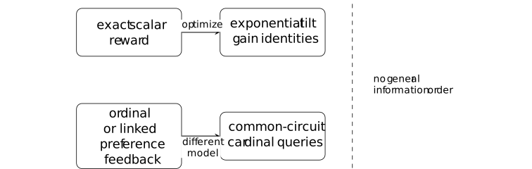
The KL identities characterize the exact optimizer for a declared scalar reward. The preference lower bounds are worst-case statements inside a fixed- circuit routing model. Bradley--Terry conclusions depend on the chosen score link. In the common-circuit specialization, cardinal queries change the information modality and admit a positive mechanism result. Outside that specialization, the preference and cardinal-query results are not directly comparable without further assumptions.
None of these statements derives the finite transcript theorem Theorem 4.4.3.5, and none proves that benchmark gain is capability acquisition. Applying either result to a training system requires that system to satisfy the corresponding information, optimizer, and comparator assumptions.
4.6. Controlled coverage, feedback resolution, and prompt breadth [ftip-009M]AGENTDRAFTED
4.6. Controlled coverage, feedback resolution, and prompt breadth [ftip-009M]AGENTDRAFTED
This section studies finite measurements and controlled comparisons that separate starting-policy coverage from the information supplied by a reward. It also records how a training prompt law limits the scope of an observed post-training effect.
The empirical route is a controlled language-model post-training study. Its reported outcomes remain experiment-specific observations. Theorems in this section follow from the stated finite-probability assumptions; the empirical results alone do not imply those conclusions.
4.6.1. Starting-policy interventions [ftip-009N]AGENTDRAFTED
4.6.1. Starting-policy interventions [ftip-009N]AGENTDRAFTED
A comparison among starting policies is meaningful only after the task, training grid, feedback rule, and evaluation procedure have been declared. Observed differences are conditional on those experimental coordinates.
Remark 4.6.1.1. The source experiment as an intervention matrix [ftip-009O]AGENTDRAFTED
Remark 4.6.1.1. The source experiment as an intervention matrix [ftip-009O]AGENTDRAFTED
[clay2026demystifying, Sections 4.1--4.3 and Figure 1] organize the reported experiments along three declared axes: a starting model distribution, a training-prompt distribution, and a reward function. Each reported measurement therefore belongs to a cell of a matrix rather than to an unqualified ``RL post-training'' condition. The source holds its broad training recipe fixed while varying selected axes; it does not study variation among RL algorithms.
Each experimental comparison is conditional on its model, task, prompt law, executable reward rule, training budget, and evaluation procedure. The reward rule is especially consequential here because the main text and Appendix C do not state identical sparse-reward semantics. Section 4.2 describes target containment with a length penalty. Appendix C's prose says an exact target receives unit reward, but its displayed equation requires the response to be strictly longer than the target for any positive reward. These two descriptions do not identify a single sparse-reward implementation.
Definition 4.6.1.2. Target-response event [ftip-009P]AGENTDRAFTED
Definition 4.6.1.2. Target-response event [ftip-009P]AGENTDRAFTED
Fix an evaluation instance \(x\), a response space \(\mathcal Y_x\), and a declared target predicate \(h_x^\star :\mathcal Y_x\to \{0,1\}\). For a sampled response \(Y\), the target-response event is
\[ E_x^\star =\{h_x^\star (Y)=1\}. \]The predicate is part of the evaluation specification. It may test exact string equality after a declared normalization, containment of a target substring, equality of a parsed answer, or another explicitly typed condition. These predicates are not interchangeable. The movie-quote and AIME experiments in [clay2026demystifying, Sections 4.1--4.2] use different response objects and therefore require different target predicates.
Remark 4.6.1.3. Exact-string success and task utility are different predicates [ftip-009Q]AGENTDRAFTED
Remark 4.6.1.3. Exact-string success and task utility are different predicates [ftip-009Q]AGENTDRAFTED
Let \(y_x^\star \) be a designated string and let \(N_x\) be a declared normalizer. Exact-string success is the specialization \(h_x^\star (y)=\mathbf 1\{N_x(y)=N_x(y_x^\star )\}\) of Definition 4.6.1.2. A task utility may instead accept semantically equivalent answers, assign partial credit, invoke a verifier, or depend on evaluator randomness as in Convention 4.1.1.
Consequently, a change in target-string match rate is not automatically a change in task utility. [clay2026demystifying, Sections 4.1--4.2] deliberately use narrow target behaviours to study controlled coverage. Transferring their measurements to broader capability requires a separately justified evaluator.
Definition 4.6.1.4. Base, SFT-positive, and SFT-negative starting-policy triple [ftip-009R]AGENTDRAFTED
Definition 4.6.1.4. Base, SFT-positive, and SFT-negative starting-policy triple [ftip-009R]AGENTDRAFTED
For one declared model family and target predicate, a starting-policy triple is
\[ \left (\pi ^{\mathrm {base}},\pi ^+,\pi ^-\right ). \]Here \(\pi ^{\mathrm {base}}\) is the unmodified starting policy, \(\pi ^+\) is obtained by a declared supervised update intended to increase target-response frequency, and \(\pi ^-\) is obtained by a declared update intended to decrease it. The superscripts name producing interventions, not mathematical order relations between the resulting policies.
[clay2026demystifying, Section 4.1] instantiates the triple with the source's Base, SFT-positive, and SFT-negative checkpoints. For the movie quote, its SFT mixture places twenty percent weight on the target quote and eighty percent on other quotes from the Cornell Movie-Dialogs corpus; the negative intervention maximizes cross-entropy loss on the target.
Remark 4.6.1.5. SFT-positive and SFT-negative are composite weight interventions [ftip-009S]AGENTDRAFTED
Remark 4.6.1.5. SFT-positive and SFT-negative are composite weight interventions [ftip-009S]AGENTDRAFTED
The policies \(\pi ^+\) and \(\pi ^-\) of Definition 4.6.1.4 are produced by optimization. Their weights, output probabilities, representations, and off-target behaviours can all change together. Calling one intervention ``positive'' and the other ``negative'' describes its intended effect on the declared target response; it does not assert that only one probability mass was edited.
The comparisons in [clay2026demystifying, Sections 4.1 and 5.1] therefore test dependence on three constructed starting checkpoints. They do not identify a causal effect of initial target probability alone without an additional intervention model.
Definition 4.6.1.6. Controlled post-training experiment cell [ftip-009T]AGENTDRAFTED
Definition 4.6.1.6. Controlled post-training experiment cell [ftip-009T]AGENTDRAFTED
A controlled post-training experiment cell is a record
\[ \mathfrak c= (M,\pi ^{\mathrm {init}},\mathsf T,\mathcal D_{\mathrm {tr}}, r^{\mathrm {id}},\mathcal A,b_{\mathrm {tr}},\mathsf E), \]where \(M\) identifies the model architecture and checkpoint lineage, \(\pi ^{\mathrm {init}}\) is its starting policy, \(\mathsf T\) is the task, \(\mathcal D_{\mathrm {tr}}\) is the training-prompt law, \(r^{\mathrm {id}}\) identifies an executable reward rule and version, \(\mathcal A\) is the update procedure, \(b_{\mathrm {tr}}\) is the training budget, and \(\mathsf E\) is the evaluation interface. Random seeds and hyperparameters belong to the relevant record fields even when suppressed from the notation.
[clay2026demystifying, Figure 1 and Sections 4.1--4.3] motivates the coordinates. The source varies starting distribution, prompt distribution, and reward while using a common broad RL setup. Because its main-text and Appendix-C sparse rewards differ, the reward field is an identifier for an executable rule, not merely the word ``sparse.''
Definition 4.6.1.7. Matched cells and held-fixed coordinates [ftip-009U]AGENTDRAFTED
Definition 4.6.1.7. Matched cells and held-fixed coordinates [ftip-009U]AGENTDRAFTED
Let \(J\) index the coordinates of an experiment cell \(\mathfrak c\) from Definition 4.6.1.6. For \(S\subseteq J\), two cells \(\mathfrak c\) and \(\mathfrak c'\) are matched outside \(S\) when
\[ \mathfrak c_j=\mathfrak c'_j\qquad \text {for every }j\in J\setminus S. \]The coordinates in \(J\setminus S\) are the held-fixed coordinates; those in \(S\) are the declared intervention coordinates. Equality means equality at the resolution recorded by the experiment, including evaluation sample size when that size affects the reported statistic.
A matched comparison licenses a contrast between the recorded cells. It does not show that a named coordinate is internally atomic. In particular, matching outside the starting-policy coordinate leaves the composite-checkpoint qualification of Remark 4.6.1.5 in force.
Example 4.6.1.8. Three starting laws under one declared training grid [ftip-009V]AGENTDRAFTED
Example 4.6.1.8. Three starting laws under one declared training grid [ftip-009V]AGENTDRAFTED
A source comparison may place the three starting policies of Definition 4.6.1.4 into cells matched outside the starting-policy coordinate. The shared boxes below mean equality of the declared grid fields, not that the three checkpoints differ in only one scalar probability.
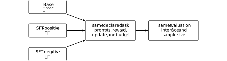
This is the comparison pattern used in [clay2026demystifying, Sections 4.1 and 5.1]. An actual cell still needs its model, task, reward implementation, and numerical record; the diagram is not a claim that all experiments in the paper instantiate one identical grid.
Remark 4.6.1.9. What the starting-policy comparison can and cannot identify [ftip-009W]AGENTDRAFTED
Remark 4.6.1.9. What the starting-policy comparison can and cannot identify [ftip-009W]AGENTDRAFTED
Within a declared model, task, training grid, and evaluation procedure, the three-cell comparison can establish that the measured post-training outcome differs across the source's constructed starting checkpoints. The movie-quote and AIME entries in [clay2026demystifying, Section 5.1, Tables 1--2] are empirical records of that form.
The comparison does not isolate initial target probability from every other SFT-induced weight change, prove that an observed zero has zero support, or establish acquisition of a broader capability. The reported model sets differ across the paper: [clay2026demystifying, Section 4.1] names OLMo 3, Qwen2-7B, Qwen3-1.7B, and Qwen2.5-7B-Instruct, while Table 1 and Appendix G also report Qwen3-8B and Qwen2-1.5B. Each measurement is specific to the model and configuration in its table row.
4.6.2. Finite initial-coverage measurement [ftip-009X]AGENTDRAFTED
4.6.2. Finite initial-coverage measurement [ftip-009X]AGENTDRAFTED
A finite evaluation records hits, not mathematical support. This subsection introduces the hit count and its sampling law, derives the exact zero-hit bound under independent sampling, and then returns to the limits of the source measurement.
Definition 4.6.2.1. Initial evaluation hit count [ftip-009Y]AGENTDRAFTED
Definition 4.6.2.1. Initial evaluation hit count [ftip-009Y]AGENTDRAFTED
Fix a starting policy, an evaluation sampling law, and the target predicate of Definition 4.6.1.2. Before post-training, draw evaluation records \((X_j,Y_j)_{j=1}^m\). Define the hit indicators and the initial evaluation hit count by
\[ I_j^\star =h_{X_j}^\star (Y_j), \qquad K_m=\sum _{j=1}^{m}I_j^\star . \]The sampling law determines whether the instances \(X_j\) are fixed, resampled, or stratified. The adjective ``initial'' locates the measurement before the post-training intervention; it does not assert that the samples are independent or that the starting policy is a foundation checkpoint.
Definition 4.6.2.2. Empirical initial success rate [ftip-009Z]AGENTDRAFTED
Definition 4.6.2.2. Empirical initial success rate [ftip-009Z]AGENTDRAFTED
For a nonempty initial evaluation sample of size \(m\), the empirical initial success rate is
\[ \widehat p_m=\frac {K_m}{m} =\widehat {\mathbb E}_{j\in \{1,\ldots ,m\}}[I_j^\star ], \]using the empirical-average convention of Convention 2.4.10. This is a statistic of the declared sample. It is not, without a sampling model and an uncertainty statement, the exact successful-support probability \(p_P(x)\) of Definition 4.3.1.
Remark 4.6.2.3. Zero observed hits are not zero probability [ftip-00A0]AGENTDRAFTED
Remark 4.6.2.3. Zero observed hits are not zero probability [ftip-00A0]AGENTDRAFTED
The equality \(K_m=0\) says that no target response occurred in one finite sample. Every success probability \(0\leq p<1\) assigns positive probability \((1-p)^m\) to this observation under independent Bernoulli sampling. Thus \(\widehat p_m=0\) does not imply \(p=0\), absence from mathematical support, or impossibility of discovery under a larger budget.
The entries printed as 0.00 percent in [clay2026demystifying, Section 5.1, Tables 1--2] are empirical rates at the stated evaluation sizes. They must not be rewritten as exact support claims.
Theorem 4.6.2.4. Zero-hit likelihood under iid evaluation [ftip-00A1]AGENTDRAFTED
Theorem 4.6.2.4. Zero-hit likelihood under iid evaluation [ftip-00A1]AGENTDRAFTED
Let \(m\in \mathbb N_{\geq 1}\). Assume the hit indicators from Definition 4.6.2.1 are independent Bernoulli variables with a common success probability \(p\). Then \(K_m\) has the binomial law and
\[ \Pr _p(K_m=0)=(1-p)^m. \]
Proof.
Proof.
The event \(K_m=0\) is \(\bigcap _{j=1}^m\{I_j^\star =0\}\). Independence and \(\Pr _p(I_j^\star =0)=1-p\) give the displayed product.
This finite statement follows from the displayed hypotheses. Applying it to a source table requires the additional iid and stationary-success assumptions stated above.
Corollary 4.6.2.5. Exact one-sided bound after zero hits [ftip-00A2]AGENTDRAFTED
Corollary 4.6.2.5. Exact one-sided bound after zero hits [ftip-00A2]AGENTDRAFTED
Assume Theorem 4.6.2.4 with \(m\in \mathbb N_{\geq 1}\) and fix \(0<\delta <1\). If \(K_m=0\), inversion of the exact zero-count likelihood gives the one-sided upper endpoint
\[ u_{m,\delta }=1-\delta ^{1/m}. \]Indeed, \(\Pr _{u_{m,\delta }}(K_m=0)=\delta \), and for every \(p>u_{m,\delta }\) one has \(\Pr _p(K_m=0)<\delta \). Thus the observed zero count excludes probabilities above \(u_{m,\delta }\) at exact level \(\delta \) under the declared iid model.
Proof.
Proof.
By Theorem 4.6.2.4, the zero-count likelihood is \((1-p)^m\), which is strictly decreasing in \(p\). Solving \((1-p)^m=\delta \) gives the endpoint and the stated strict inequality.
This is a likelihood inversion derived from the displayed finite setup, not a source theorem and not a support certificate.
Example 4.6.2.6. The 128-sample zero-hit bound [ftip-00A3]AGENTDRAFTED
Example 4.6.2.6. The 128-sample zero-hit bound [ftip-00A3]AGENTDRAFTED
Take \(m=128\) and \(\delta =0.05\) in Corollary 4.6.2.5. After zero hits, the exact one-sided upper endpoint is
\[ u_{128,0.05} =1-0.05^{1/128} \approx 0.02313. \]Under the iid Bernoulli model, probabilities above approximately 2.313 percent make a zero count less than five percent likely. The calculation does not turn a recorded \(0/128\) into proof that the true probability is zero, and it does not apply if the 128 evaluations have a different joint sampling law.
Definition 4.6.2.7. First positive sparse-reward time [ftip-00A4]AGENTDRAFTED
Definition 4.6.2.7. First positive sparse-reward time [ftip-00A4]AGENTDRAFTED
Fix an executable sparse-reward rule and let \(r_j^{\mathrm {sp}}\) be the reward returned on rollout \(j\). The first positive sparse-reward time is the extended-valued index
\[ J_+=\inf \{j\geq 1:r_j^{\mathrm {sp}}>0\}, \qquad \inf \varnothing :=\infty . \]This definition concerns the reward implementation named by an experiment cell. The event \(r_j^{\mathrm {sp}}>0\) coincides with a target-response event only when that equality is part of the declared reward semantics. In particular, a length penalty or partial-credit rule can separate positive reward from exact target match.
Corollary 4.6.2.8. Sparse-reward discovery within a rollout budget [ftip-00A5]AGENTDRAFTED
Corollary 4.6.2.8. Sparse-reward discovery within a rollout budget [ftip-00A5]AGENTDRAFTED
Suppose the events \(\{r_j^{\mathrm {sp}}>0\}\) are independent and have a common probability \(q\). For every positive rollout budget \(B\),
\[ \Pr (J_+\leq B)=1-(1-q)^B. \]
Proof.
Proof.
Apply the independent-attempt theorem Theorem 4.4.1.2 with \(E_j=\{r_j^{\mathrm {sp}}>0\}\). Its discovery event is exactly \(\{J_+\leq B\}\).
This is a specialization proved from the displayed hypotheses. It does not supply independence, stationarity, or the value of \(q\) for a training run, and it does not equate positive proxy reward with task utility.
Example 4.6.2.9. The AIME 128-sample measurement record [ftip-00A6]AGENTDRAFTED
Example 4.6.2.9. The AIME 128-sample measurement record [ftip-00A6]AGENTDRAFTED
[clay2026demystifying, Section 5.1, Table 2] reports the following empirical target-answer rates for AIME Problem 4 with Qwen2.5-7B-Instruct and evaluation size \(m=128\). The task asks for the number of integer pairs \((x,y)\in [-100,100]^2\) satisfying \(12x^2-xy-6y^2=0\); the target answer is \(117\).
\[ \begin {array}{c|ccc} &\mathrm {SFT{+}}&\mathrm {Base}&\mathrm {SFT{-}}\\ \hline \text {No Reward}&26.6&3.92&0.00\\ \text {Sparse Reward}&85.9&10.2&0.00\\ \text {Dense Reward}&86.7&92.2&0.00 \end {array} \]Every entry in the displayed array is a percentage.
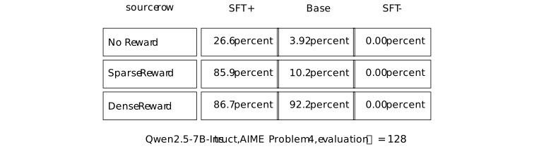
These are source-reported empirical percentages, not exact policy probabilities. ``No Reward'' is retained as the source's row label; the table alone does not define it as a post-training protocol. The three zero entries for SFT-negative are finite observations and remain subject to Remark 4.6.2.3. Appendix Figure 5's caption prints a different set of Qwen2.5-7B-Instruct values that duplicates the neighbouring movie-quote caption and is incompatible with Table 2. The displayed percentages are those of Table 2; the caption does not provide a consistent alternative measurement.
Remark 4.6.2.10. An observed plateau is not a universal probability threshold [ftip-00A7]AGENTDRAFTED
Remark 4.6.2.10. An observed plateau is not a universal probability threshold [ftip-00A7]AGENTDRAFTED
[clay2026demystifying, Section 5.2 and Figure 2] report that the Qwen3-1.7B Base movie-quote cell, whose initial empirical match rate is about 0.5 percent, does not optimize under the source's sparse-reward run, whereas its dense-reward run rises toward fifty percent. [clay2026demystifying, Appendix Figure 8] gives final match rates 10.0 percent for sparse reward and 48.8 percent for dense reward. Thus ``failed'' here means failure of the reported sparse run to optimize as intended, not zero final matches.
A plateau is indexed by the model, target, reward implementation, optimizer, sampling process, and budget in its experiment cell. One observed transition therefore does not identify a universal initial-probability threshold for RL learning, support, or capability acquisition.
4.6.3. Sparse, dense, and process feedback [ftip-00A8]AGENTDRAFTED
4.6.3. Sparse, dense, and process feedback [ftip-00A8]AGENTDRAFTED
Sparse, dense, and process rewards expose different observations about a response. This subsection treats that difference as a change in the feedback channel, rather than as a free change in the smoothness of one fixed objective.
Definition 4.6.3.1. Sparse exact reward [ftip-00A9]AGENTDRAFTED
Definition 4.6.3.1. Sparse exact reward [ftip-00A9]AGENTDRAFTED
Let \(\mathcal Y\) be a finite response set and fix a target response \(\tau \in \mathcal Y\). The sparse exact reward is the map \(r_{\rm exact}:\mathcal Y\to \{0,1\}\) defined by
\[ r_{\rm exact}(y)=\mathbf 1\{y=\tau \}. \]This idealized reward exposes one bit: whether the whole response equals the target. It does not expose a prefix, edit location, or partial milestone. The movie-quote source uses related but textually inconsistent substring and length-penalized rewards; the distinct formulas are compared in Remark 4.6.3.2.
Remark 4.6.3.2. Main-text and Appendix-C sparse-reward discrepancy [ftip-00AA]AGENTDRAFTED
Remark 4.6.3.2. Main-text and Appendix-C sparse-reward discrepancy [ftip-00AA]AGENTDRAFTED
Section 4.2 of Demystifying Reinforcement Learning Post-Training of Language Models[clay2026demystifying] displays a substring indicator \(\mathbf 1\{\tau \subseteq y\}\) and says that a length penalty is applied. In Appendix C, \(n\) is the maximum generation length and \(s\) is the number of tokens beyond the target. The appendix first defines the excess-length penalty
\[ p(s)= \begin {cases} 0,&s=0,\\ s/n,&s>0, \end {cases} \]and then gives Equation (3):
\[ r_{\rm C}(y,\tau )= \begin {cases} \max \{0.5,1-p(s)\},&\tau \text { occurs in }y \text { and }|y|>|\tau |,\\ 0,&\text {otherwise}. \end {cases} \]As printed, Equation (3) assigns zero when \(y=\tau \), because its first branch requires strict excess length. This conflicts with the immediately preceding Appendix-C prose, which assigns base reward one when the target is generated, and it is not the exact-match reward of Definition 4.6.3.1. The two printed descriptions therefore specify different reward rules.
Definition 4.6.3.3. Edit-distance reward [ftip-00AB]AGENTDRAFTED
Definition 4.6.3.3. Edit-distance reward [ftip-00AB]AGENTDRAFTED
Let \(y=y_1\cdots y_m\) and a nonempty target \(\tau =\tau _1\cdots \tau _n\) be finite strings. Their Levenshtein distance is determined by \(D(0,j)=j\), \(D(i,0)=i\), and, for \(i,j>0\),
\[ D(i,j)=\min \left \{ \begin {aligned} &D(i-1,j)+1,\\ &D(i,j-1)+1,\\ &D(i-1,j-1)+\mathbf 1\{y_i\neq \tau _j\} \end {aligned} \right \}. \]Set \(L(y,\tau )=\max \{|y|,|\tau |\}\). The edit-distance reward is
\[ r_{\rm edit}(y,\tau ) =\max \left \{0,1-\frac {D(|y|,|\tau |)}{L(y,\tau )}\right \}. \]The recurrence is Equation (1) in the main text and Equation (4) in Appendix C of Demystifying Reinforcement Learning Post-Training of Language Models[clay2026demystifying]; the normalized reward is its Equation (5). The nonempty-target assumption makes the displayed denominator positive. This reward does not establish that edit similarity is the correct utility for a different task.
Remark 4.6.3.4. Dense reward imports target structure [ftip-00AC]AGENTDRAFTED
Remark 4.6.3.4. Dense reward imports target structure [ftip-00AC]AGENTDRAFTED
The edit reward of Definition 4.6.3.3 is not obtained from the binary value in Definition 4.6.3.1 by a numerical smoothing operation. It also receives the target string, a character-level edit model, and the ordering of symbols. Two non-target responses that both receive sparse reward zero can therefore receive different edit rewards.
That extra resolution can improve credit assignment, but it changes the feedback channel and its assumptions. The source calls edit distance a dense proxy and reports controlled movie-quote experiments [clay2026demystifying, Sections 4.2 and 5.2]. Neither the formula nor those observations establish that edit proximity is an independent measure of general response quality.
Definition 4.6.3.5. Milestone process reward [ftip-00AD]AGENTDRAFTED
Definition 4.6.3.5. Milestone process reward [ftip-00AD]AGENTDRAFTED
For the source's fixed AIME problem, let
\[ M(y)=(m_1(y),\ldots ,m_5(y))\in \{0,1\}^5 \]record whether a completed response contains five declared milestones: a valid algebraic setup, correct root relations, correct integer bounds, a correct count for at least one branch, and correct subtraction of the overlap at the origin. With
\[ (w_1,\ldots ,w_5)=(0.05,0.05,0.10,0.15,0.25), \]the milestone process reward is
\[ r_{\rm proc}(y)=\sum _{i=1}^{5}w_i m_i(y). \]Appendix D.1 of Demystifying Reinforcement Learning Post-Training of Language Models[clay2026demystifying] gives Equation (6) and the milestone list above. In the experiment, a 32-billion-parameter instruction-tuned model classifies the completed trajectory. The displayed map is therefore richer than a deterministic final-answer verifier, even though it returns one scalar after the rollout.
Remark 4.6.3.6. Process feedback assumptions and milestone-weight discrepancy [ftip-00AE]AGENTDRAFTED
Remark 4.6.3.6. Process feedback assumptions and milestone-weight discrepancy [ftip-00AE]AGENTDRAFTED
Appendix D.2 of Demystifying Reinforcement Learning Post-Training of Language Models[clay2026demystifying] supplements \(r_{\rm proc}\) with an extracted-answer override and two penalties. Translating its notation, let \(\tau =117\), \(\tau _{\rm near}=118\), and define
\[ r_{\rm base}(y)= \begin {cases} 1.0,&\operatorname {extract}(y)=\tau ,\\ 0.6,&\operatorname {extract}(y)=\tau _{\rm near},\\ r_{\rm proc}(y),&\text {otherwise}. \end {cases} \]Let \(p_{\rm loop}(y)=-0.3\) when the judge flags a loop without the exact answer, and zero otherwise. Let \(p_{\rm format}(y)=-0.5\) when the response lacks the required boxed delimiter, and zero otherwise. Equations (7)--(8) then give
\[ r_{\rm PRM}(y) =\max \{0,r_{\rm base}(y)+p_{\rm loop}(y)+p_{\rm format}(y)\}. \]These clauses assume a reliable milestone judge, parser, near-miss choice, loop flag, and formatting rule. They are part of the feedback definition, not consequences of reinforcement learning. The main text describes ``exponentially increasing'' dense rewards, and Appendix D calls the weights ``exponential scaling.'' The printed vector \((0.05,0.05,0.10,0.15,0.25)\) is neither strictly increasing at every milestone nor a geometric progression. We preserve the exact weights and do not infer an exponential law from that wording.
Definition 4.6.3.7. Reward-induced observational equivalence [ftip-00AF]AGENTDRAFTED
Definition 4.6.3.7. Reward-induced observational equivalence [ftip-00AF]AGENTDRAFTED
Let \(\mathcal Y\) be a finite response set and \(r:\mathcal Y\to \mathcal R\) any reward map. Two responses are observationally equivalent under \(r\), written \(y\sim _r y'\), when
\[ y\sim _r y'\quad \Longleftrightarrow \quad r(y)=r(y'). \]Equality makes \(\sim _r\) an equivalence relation. Its quotient \(\mathcal Y/{\sim _r}\) is the finite set of response classes distinguished by the reward alone. This proposed equivalence relation ignores any information in the response that is not returned by \(r\); equal rewards need not imply equal latent utility.
Lemma 4.6.3.8. Refining feedback separates at least as many responses [ftip-00AG]AGENTDRAFTED
Lemma 4.6.3.8. Refining feedback separates at least as many responses [ftip-00AG]AGENTDRAFTED
Let \(\mathcal Y\) be finite and let \(r_1:\mathcal Y\to \mathcal R_1\) and \(r_2:\mathcal Y\to \mathcal R_2\). Say that \(r_2\) refines \(r_1\) when
\[ r_2(y)=r_2(y')\quad \Longrightarrow \quad r_1(y)=r_1(y') \qquad (y,y'\in \mathcal Y). \]If \(r_2\) refines \(r_1\), then
\[ \left |\mathcal Y/{\sim _{r_2}}\right | \geq \left |\mathcal Y/{\sim _{r_1}}\right |. \]
Proof.
Proof.
Send the \(r_2\)-class of \(y\) to the \(r_1\)-class of \(y\). The refinement condition makes this map well defined. It is surjective because every \(r_1\)-class contains some \(y\), whose \(r_2\)-class maps to it. A surjection between finite sets has a domain at least as large as its codomain.
This finite lemma compares observational partitions only. It does not say that the refined reward is cheaper, more accurate, or better aligned with utility.
Example 4.6.3.9. Counterexample: equal sparse reward, unequal dense reward [ftip-00AH]AGENTDRAFTED
Example 4.6.3.9. Counterexample: equal sparse reward, unequal dense reward [ftip-00AH]AGENTDRAFTED
Take the target string \(\tau =\texttt {abc}\) and two responses \(y=\texttt {abx}\) and \(y'=\texttt {xyz}\). Both fail exact matching, while their edit distances and normalized edit rewards are
\[ \begin {array}{c|c|c|c} \text {response}&r_{\rm exact}&D(\,cdot\,,\tau )&r_{\rm edit}\\ \hline \texttt {abx}&0&1&2/3\\ \texttt {xyz}&0&3&0 \end {array} \]Thus \(y\sim _{r_{\rm exact}}y'\) but \(y\not \sim _{r_{\rm edit}}y'\). The example witnesses a strict separation inside one sparse-reward class. It does not claim that every dense proxy refines every sparse verifier.
Example 4.6.3.10. Three feedback resolutions on one response set [ftip-00AI]AGENTDRAFTED
Example 4.6.3.10. Three feedback resolutions on one response set [ftip-00AI]AGENTDRAFTED
One finite response set can be observed through three different maps. The arrows below share a domain; they do not assert that the three codomains form a refinement chain.
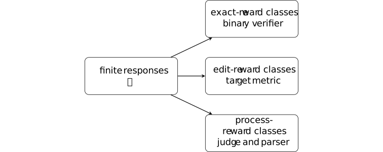
The exact reward forgets every difference among failures. Edit reward can retain character-level proximity, while the source process reward retains a declared milestone vector only after judge, override, and penalty choices. The partition lemma Lemma 4.6.3.8 applies to a pair only after its refinement hypothesis has been checked.
Remark 4.6.3.11. Reward density is not cost-free smoothing [ftip-00AJ]AGENTDRAFTED
Remark 4.6.3.11. Reward density is not cost-free smoothing [ftip-00AJ]AGENTDRAFTED
A denser reward can distinguish more responses and supply more frequent update signal. It can also require information absent from a sparse verifier. In the controlled source, edit feedback assumes the full target and computes a string metric; process feedback uses a 32-billion-parameter judge, five problem-specific milestones, answer extraction, an enumerated near miss, and loop and format penalties [clay2026demystifying, Appendices C--D].
The richer feedback channel incurs specification, computation, and validation costs. Replacing sparse feedback by dense feedback can alter both the information available to training and the objective being optimized. The resulting comparison is an intervention on feedback resolution, not evidence that one fixed reward was smoothed at zero cost.
4.6.4. Prompt breadth and effect locality [ftip-00AK]AGENTDRAFTED
4.6.4. Prompt breadth and effect locality [ftip-00AK]AGENTDRAFTED
Training on one prompt law can change behavior unevenly across evaluation slices. Localized and distributed degradation are distinguished relative to that training law and the specified evaluation slices.
Definition 4.6.4.1. Training prompt law and evaluated prompt slice [ftip-00AL]AGENTDRAFTED
Definition 4.6.4.1. Training prompt law and evaluated prompt slice [ftip-00AL]AGENTDRAFTED
Let \(\mathcal X\) be a task-instance set. Write \(\mu _{\rm tr}=\mathcal D_{\rm tr}\) for the training-prompt coordinate of an experiment cell in Definition 4.6.1.6. A training prompt law is this probability law on \(\mathcal X\), used to draw instances during a post-training protocol. Let \(\mu _{\rm ev}\) be an independently declared evaluation law on the same set.
An evaluated prompt slice is a measurable set \(C\subseteq \mathcal X\) with \(\mu _{\rm ev}(C)>0\). Its conditional evaluation law is
\[ \mu _{\rm ev}(A\mid C) =\frac {\mu _{\rm ev}(A\cap C)}{\mu _{\rm ev}(C)}. \]The training and evaluation laws need not agree. A slice records where an effect is measured; it does not assert that prompts inside the slice are equally difficult or represented equally in pretraining. We specialize the task-law convention of Definition 1.4.3.
Definition 4.6.4.2. Source-specific narrow and broad configurations [ftip-00AM]AGENTDRAFTED
Definition 4.6.4.2. Source-specific narrow and broad configurations [ftip-00AM]AGENTDRAFTED
A prompt configuration is the record
\[ \mathsf c=(M_0,\mu _{\rm tr},m_{\rm tr},r,\mathsf A,b), \]containing the starting artifact, training prompt law, finite prompt-pool size, reward, update algorithm, and training budget. We call two particular records \(\mathsf c_{\rm nar}\) and \(\mathsf c_{\rm brd}\) only when a cited experiment names them narrow and broad.
Section 4.3 and Appendix F of Demystifying Reinforcement Learning Post-Training of Language Models[clay2026demystifying] instantiate these labels in two model-family experiments. The Qwen comparison uses 100 DeepScaleR prompts versus 10,000 WildChat prompts. The OLMo comparison uses 100 math-only prompts versus 10,000 prompts split evenly among mathematics, instruction following, and code. These labels identify the two reported configurations; they do not define a general measure or ordering of prompt breadth.
Remark 4.6.4.3. Prompt breadth is not a total order [ftip-00AN]AGENTDRAFTED
Remark 4.6.4.3. Prompt breadth is not a total order [ftip-00AN]AGENTDRAFTED
The records in Definition 4.6.4.2 change several coordinates together. The prompt-pool size, domain mixture, and repetition frequency differ. Across the paper's Qwen and OLMo studies, the starting artifact and evaluated tasks also differ.
We therefore use ``narrow'' and ``broad'' as names for the source cells. They do not define a total order on prompt laws, and their comparison does not identify a causal effect of breadth alone. A breadth theorem would need a declared statistic and matched configurations that differ only in that statistic.
Definition 4.6.4.4. Slice-conditioned success change [ftip-00AO]AGENTDRAFTED
Definition 4.6.4.4. Slice-conditioned success change [ftip-00AO]AGENTDRAFTED
Fix an evaluated slice \(C\) from Definition 4.6.4.1, and let \(P_0\) and \(P_1\) denote the pre- and post-training protocols whose successful-support probabilities are defined in Definition 4.3.1. The slice-conditioned success change is
\[ \Delta _{\rm suc}(C;P_1,P_0) =\mathbb E_{X\sim \mu _{\rm ev}(\cdot \mid C)} \left [p_{P_1}(X)-p_{P_0}(X)\right ]. \]The evaluation interface, inference budget, and success predicate are held fixed across the two terms. The quantity is an average change on one declared slice. It neither locates the change inside the model nor identifies which training coordinate caused it.
Definition 4.6.4.5. Localized and distributed degradation [ftip-00AP]AGENTDRAFTED
Definition 4.6.4.5. Localized and distributed degradation [ftip-00AP]AGENTDRAFTED
Fix pairwise disjoint evaluated slices \(C_1,\ldots ,C_J\) and a declared degradation threshold \(\kappa >0\). Define the set of materially degraded slices
\[ \mathcal H_\kappa (P_1,P_0) =\left \{j:\Delta _{\rm suc}(C_j;P_1,P_0)\leq -\kappa \right \}. \]Degradation is localized relative to this slice family and threshold when \(|\mathcal H_\kappa |=1\). It is distributed when \(|\mathcal H_\kappa |\geq 2\).
These terms depend on the chosen partition, threshold, and evaluation budget. They do not turn a finite benchmark vector into a statement about all capabilities.
Example 4.6.4.6. Narrow and broad random-reward paths [ftip-00AQ]AGENTDRAFTED
Example 4.6.4.6. Narrow and broad random-reward paths [ftip-00AQ]AGENTDRAFTED
Section 5.3 and Appendix F of Demystifying Reinforcement Learning Post-Training of Language Models[clay2026demystifying] supply two OLMo paths; Figure 4 reports their outcomes. Both replace the usual verifiable reward with a random scalar drawn from \(\operatorname {Unif}[0,1]\), but their prompt configurations differ.
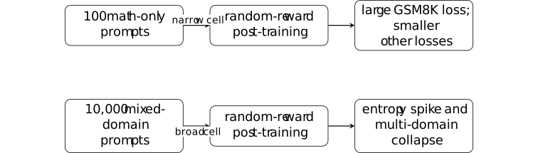
In the narrow SFT-start path, GSM8K accuracy falls from 86 to about 32 by step 400, while the reported MMLU and IFEval changes are much smaller. In the broad path, the source reports an entropy spike near step 400 together with collapse on GSM8K, MMLU, and IFEval. The diagram records that interpretation; it does not isolate prompt breadth from pool size, mixture, or repetition.
Remark 4.6.4.7. What the source observes about spurious reward [ftip-00AR]AGENTDRAFTED
Remark 4.6.4.7. What the source observes about spurious reward [ftip-00AR]AGENTDRAFTED
Section 5.3 and Figures 3--4 of Demystifying Reinforcement Learning Post-Training of Language Models[clay2026demystifying] report that the Qwen narrow configuration retains higher MATH and AMC Acc@1 than its broad configuration under random reward. The OLMo experiment reports the different evaluation patterns summarized in Example 4.6.4.6.
These are finite empirical observations. The random scalar reward removes task alignment from one feedback channel, but it does not hold all other training coordinates fixed. The reported entropy is a named token statistic, not a direct measure of capability or acquisition.
Example 4.6.4.8. Counterexample: equal marginal reward, unequal prompt-local damage [ftip-00AS]AGENTDRAFTED
Example 4.6.4.8. Counterexample: equal marginal reward, unequal prompt-local damage [ftip-00AS]AGENTDRAFTED
Let two evaluation slices \(C_1,C_2\) have equal mass. A feedback channel returns an independent Bernoulli reward with mean \(1/2\) under either of two post-training protocols. Suppose their fixed-interface success changes are
\[ \left (\Delta _{\rm suc}(C_1),\Delta _{\rm suc}(C_2)\right ) =(-1,0) \quad \hbox {or}\quad \left (-\tfrac 12,-\tfrac 12\right ). \]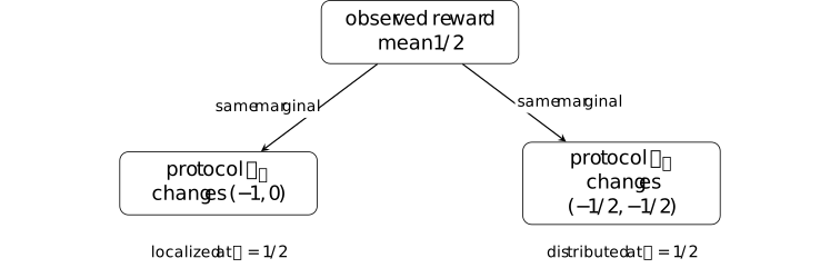
The reward law and its mean are identical, but the slice-level evaluation vectors differ. Hence marginal training reward does not determine whether damage is localized or distributed. This is a finite counterexample, not a claim about the mechanism in the source experiment.
Remark 4.6.4.9. Coverage, feedback resolution, and prompt-conditioned effects [ftip-00AT]AGENTDRAFTED
Remark 4.6.4.9. Coverage, feedback resolution, and prompt-conditioned effects [ftip-00AT]AGENTDRAFTED
The source cells motivate tests of starting-policy coverage, feedback resolution, and prompt-conditioned damage. They do not establish that dense reward creates mathematical support, that zero sampled hits imply zero probability, or that random reward has one model-independent effect.
Separating the effects of coverage, feedback resolution, and prompt breadth requires stronger controls. One comparison fixes prompt laws and varies only the feedback sigma-algebra. Another fixes feedback and evaluation while varying one starting-policy coordinate. Confidence regions for the complete vector of slice-conditioned changes would quantify effects that an aggregate score can hide.
The reported observations remain conditional on their experimental configurations. They do not establish general results about capability acquisition, elicitation, or the optimal allocation of post-training compute.
4.7. Finite consequences and counterexamples [ftip-00JE]AGENTDRAFTED
4.7. Finite consequences and counterexamples [ftip-00JE]AGENTDRAFTED
Finite sampling, reward information, and deterministic execution give conditional conclusions about post-training. Their counterexamples show why the task law, feasible set, and available information cannot be omitted.
This synthesis brings together the finite results used in the evaluation analysis. The conceptual-discovery chapter asks whether such arguments can constrain a complete learning lineage, including changes to representations, curricula and research procedures.
4.7.1. Probability, information, and execution [ftip-00I1]AGENTDRAFTED
4.7.1. Probability, information, and execution [ftip-00I1]AGENTDRAFTED
Discovery probabilities, support, proxy error, feedback resolution, and replay each constrain a different part of a comparison. Capability remains conditional behavior under a declared intervention and evaluation law, rather than a scalar latent property.
4.7.1.1. Finite probability and execution results [ftip-00I2]AGENTDRAFTED
4.7.1.1. Finite probability and execution results [ftip-00I2]AGENTDRAFTED
The conclusions depend on their declared probability laws, finite index sets, positivity conditions, and execution inputs. Changing one of these assumptions can change the result even when the observed score is unchanged.
Convention 4.7.1.1.1. Domains of the finite results [ftip-00I5]AGENTDRAFTED
Convention 4.7.1.1.1. Domains of the finite results [ftip-00I5]AGENTDRAFTED
Each result concerns its declared carriers \(X_1,\ldots ,X_n\), with fixed equality and order conventions. Finiteness, probability laws, and positivity conditions are hypotheses of the result; they cannot be inferred from a finite observation alone.
Theorem 4.7.1.1.2. Independent discovery probability [ftip-00I7]AGENTDRAFTED
Theorem 4.7.1.1.2. Independent discovery probability [ftip-00I7]AGENTDRAFTED
For \(B\in \mathbb N\) independent discovery events with the probabilities declared in Convention 4.4.1.1, the identity in Theorem 4.4.1.2 gives \(\Pr (D_B)=1-\prod _{i=1}^{B}(1-p_i)\).
Theorem 4.7.1.1.3. Discovery budget for a failure threshold [ftip-00I8]AGENTDRAFTED
Theorem 4.7.1.1.3. Discovery budget for a failure threshold [ftip-00I8]AGENTDRAFTED
Under \(0<p<1\), \(0<\delta <1\), and an integer budget \(B\geq 1\), the failure constraint is equivalent to the following bound.
\[B\geq \left \lceil \frac {\log \delta }{\log (1-p)}\right \rceil .\]The result is proved in Corollary 4.4.1.3.
Theorem 4.7.1.1.4. Support under finite exponential tilting [ftip-00I9]AGENTDRAFTED
Theorem 4.7.1.1.4. Support under finite exponential tilting [ftip-00I9]AGENTDRAFTED
Under the finite-carrier and positive-temperature hypotheses of Theorem 4.4.1.6, normalized exponential tilting preserves the base law's positive support.
Theorem 4.7.1.1.5. Uniform proxy error and objective regret [ftip-00IA]AGENTDRAFTED
Theorem 4.7.1.1.5. Uniform proxy error and objective regret [ftip-00IA]AGENTDRAFTED
For a finite common feasible set and a common regularizer, the uniform proxy error hypothesis in Definition 4.4.2.1 yields the two-epsilon objective regret bound proved in Theorem 4.4.2.2; the conclusion concerns the regularized objective named there.
Theorem 4.7.1.1.6. Utility under a change of evaluation law [ftip-00IB]AGENTDRAFTED
Theorem 4.7.1.1.6. Utility under a change of evaluation law [ftip-00IB]AGENTDRAFTED
If the evaluation laws and finite response space satisfy the total-variation hypotheses of Theorem 4.2.5.2, then the expectation difference is bounded by the stated sup-norm times total variation.
Theorem 4.7.1.1.7. Response classes under feedback refinement [ftip-00IC]AGENTDRAFTED
Theorem 4.7.1.1.7. Response classes under feedback refinement [ftip-00IC]AGENTDRAFTED
For finite response set \(\mathcal Y\) and deterministic rewards, a reward channel that refines the equality partition of another channel separates at least as many response classes, as proved in Lemma 4.6.3.8.
Theorem 4.7.1.1.8. Equal execution inputs give equal replay traces [ftip-00IJ]AGENTDRAFTED
Theorem 4.7.1.1.8. Equal execution inputs give equal replay traces [ftip-00IJ]AGENTDRAFTED
If the execution map is deterministic in all coordinates fixed by Definition 3.5.3.5, then equal input, revision, environment, and seed records produce equal finite traces, as proved in Theorem 3.5.3.6.
Theorem 4.7.1.1.9. Observational equivalence under a common update kernel [ftip-00IK]AGENTDRAFTED
Theorem 4.7.1.1.9. Observational equivalence under a common update kernel [ftip-00IK]AGENTDRAFTED
For the finite transcript and world kernels declared in Definition 4.4.3.2--Definition 4.4.3.3, observationally equivalent worlds induce the same output law for any common randomized post-training kernel, as proved in Theorem 4.4.3.5.
Theorem 4.7.1.1.10. Conditions for an admissible commit decision [ftip-00IL]AGENTDRAFTED
Theorem 4.7.1.1.10. Conditions for an admissible commit decision [ftip-00IL]AGENTDRAFTED
Under the typed audit record of Definition 3.5.4.1, a commit is admissible exactly when all required checks pass, the digest matches, and the recorded decision is \(commit\), as proved in Theorem 3.5.4.2.
Theorem 4.7.1.1.11. Admission of a finite audit plan [ftip-00IM]AGENTDRAFTED
Theorem 4.7.1.1.11. Admission of a finite audit plan [ftip-00IM]AGENTDRAFTED
A finite audit plan with nonnegative stage costs is admissible exactly when its declared additive cost is within budget; adding a positive stage beyond slack is inadmissible, by Theorem 3.5.5.4.
4.7.1.2. Counterexamples and restricted assumptions [ftip-00ID]AGENTDRAFTED
4.7.1.2. Counterexamples and restricted assumptions [ftip-00ID]AGENTDRAFTED
Finite constructions can separate average success from coverage, proxy accuracy from evaluation quality, and observed gradients from the hypotheses needed to bound them. Each separation identifies an assumption that a stronger conclusion would require.
Remark 4.7.1.2.1. What a finite counterexample establishes [ftip-00IE]AGENTDRAFTED
Remark 4.7.1.2.1. What a finite counterexample establishes [ftip-00IE]AGENTDRAFTED
A finite assignment satisfying a claim's hypotheses and violating its conclusion disproves that universal claim. It does not estimate how often the failure occurs under another distribution or establish a general failure rate.
Remark 4.7.1.2.2. Changing the model or evaluation changes the claim [ftip-00IF]AGENTDRAFTED
Remark 4.7.1.2.2. Changing the model or evaluation changes the claim [ftip-00IF]AGENTDRAFTED
A conclusion about fixed carriers, policies, feedback, budgets, and evaluation laws need not survive a change to those objects. Finite zero hits do not imply zero support, empirical benchmark movement does not imply acquisition, and an exact-optimizer result need not hold for an approximate optimizer without an additional error bound.
Example 4.7.1.2.3. Equal averages and zero hits do not identify coverage [ftip-00IG]AGENTDRAFTED
Example 4.7.1.2.3. Equal averages and zero hits do not identify coverage [ftip-00IG]AGENTDRAFTED
The two-task examples in Example 4.4.1.8 and Example 4.6.2.6 show that equal one-shot averages or zero observed hits can coexist with different coverage or nonzero latent rates. These conclusions use their declared iid model and do not estimate rates outside it.
Example 4.7.1.2.4. Small training-law error can reverse evaluation selection [ftip-00IH]AGENTDRAFTED
Example 4.7.1.2.4. Small training-law error can reverse evaluation selection [ftip-00IH]AGENTDRAFTED
In the two-point construction of Example 4.4.2.4, training-law average error is small while evaluation selection reverses. The missing hypothesis is a uniform bound on the evaluated feasible set; an informal promise of similar distributions does not supply it.
Remark 4.7.1.2.5. Untied heads, shared gradients, and checkpoint forecasts [ftip-00II]AGENTDRAFTED
Remark 4.7.1.2.5. Untied heads, shared gradients, and checkpoint forecasts [ftip-00II]AGENTDRAFTED
For DGG, the untied head identity and its finite-batch Jensen bound in Theorem 4.4.4.1 and Theorem 4.4.4.3 differ from an intermediate-occurrence bound. A shared intermediate weight requires the sum over all occurrences in Theorem 4.4.4.1; the source's local hypotheses do not establish its claimed total-gradient bound in [miao2026when, Section 4.2.1, Lemma 1, Theorem 1, and Appendix A.3]. The cancellation example Example 4.4.4.6 also separates the active clipping interval from the raw-surrogate extension.
NExt's empirical checkpoint forecasts in [chen2026lowrank, Sections 3.2, 4.1--4.3, and 5.1] do not establish a universal subspace-collapse, capability, or speed theorem. The spectral and evaluation quantities in Definition 4.4.4.8 through Remark 4.4.4.13 measure different trajectory properties.
4.7.1.3. Mathematical notation [ftip-00IN]AGENTDRAFTED
4.7.1.3. Mathematical notation [ftip-00IN]AGENTDRAFTED
Prompt and response spaces, probability laws, policies, rewards, evaluation scores, and execution traces are distinct mathematical objects.
Convention 4.7.1.3.1. Prompt spaces, response spaces, and laws [ftip-00IO]AGENTDRAFTED
Convention 4.7.1.3.1. Prompt spaces, response spaces, and laws [ftip-00IO]AGENTDRAFTED
Use \(\mathcal X\) for prompts, \(\mathcal Y\) for finite responses, \(\Omega \) for sample space, \(\mathsf P\) for a declared protocol, and \(\mu \) for a prompt law. A probability law is written \(\Pr \) only after its sample space is named.
Convention 4.7.1.3.2. Policies and reference policies [ftip-00IP]AGENTDRAFTED
Convention 4.7.1.3.2. Policies and reference policies [ftip-00IP]AGENTDRAFTED
Use \(\pi \) for a policy, \(\pi _{\rm base}\) for a reference policy, and \(\pi _\theta \) for a parameterized policy. A policy is always typed as a kernel from the declared prompt carrier to the declared response carrier.
Convention 4.7.1.3.3. Rewards and evaluation utilities [ftip-00IQ]AGENTDRAFTED
Convention 4.7.1.3.3. Rewards and evaluation utilities [ftip-00IQ]AGENTDRAFTED
Use \(r:\mathcal X\times \mathcal Y\to \mathbb R\) for a deterministic reward and \(u\) for an evaluation utility. Proxy, verifier, and process rewards retain their local subscripts; no bare symbol silently changes meaning.
Convention 4.7.1.3.4. Model artifacts and evaluation scores [ftip-00IR]AGENTDRAFTED
Convention 4.7.1.3.4. Model artifacts and evaluation scores [ftip-00IR]AGENTDRAFTED
Use \(M\) for a model artifact, \(\mathsf E\) for an evaluation protocol, and \(J_{\mathsf E}(M)\) for its declared score. A comparison must state the invariant evaluation law before subtracting two scores.
Convention 4.7.1.3.5. Traces, states, lineages, and costs [ftip-00IS]AGENTDRAFTED
Convention 4.7.1.3.5. Traces, states, lineages, and costs [ftip-00IS]AGENTDRAFTED
Use \(z_{0:n}\) for a finite trace, \(s_t\) for a harness state, \(\ell \) for a lineage, and \(c\) for an execution cost. Event logs and summaries are distinct carriers even when one is computed from the other.
5. Architecture-conditioned potential and computation [ftip-00JC]AGENTDRAFTED
5. Architecture-conditioned potential and computation [ftip-00JC]AGENTDRAFTED
This chapter refines the evaluation framework for claims that depend on architecture, optimization geometry or a systems implementation. It begins with the decoder-only Transformer, then maps mechanism families to capability bottlenecks before introducing architecture-indexed frontiers and matched-compute comparisons. It also studies how an optimizer can depend on the representation of its parameters.
The reference architecture specifies how token probabilities are computed; it does not replace the shared task and evaluation interfaces. The mechanism-family map asks which bottleneck a design changes and what evidence would demonstrate that change; it does not rank model families. Readers whose question does not depend on an architecture or optimizer can continue directly to conceptual discovery. Changes to retained context and rollout computation are treated with agent state.
5.1. Decoder-only Transformer architecture [ftip-000K]AGENTDRAFTED
5.1. Decoder-only Transformer architecture [ftip-000K]AGENTDRAFTED
The continuation law in Definition 1.2.9 specifies what probabilities a language model exposes. A decoder-only Transformer specifies how a sequence of token identifiers is transformed into those probabilities. This section introduces one component at a time, with dimensions fixed before the component formulas are used.
Notation 5.1.1. Tensor dimensions, positions, heads, and layers [ftip-000L]AGENTDRAFTED
Notation 5.1.1. Tensor dimensions, positions, heads, and layers [ftip-000L]AGENTDRAFTED
Let \(T\) be the maximum token positions processed together, \(d\) the residual-stream width, \(d_{\mathrm {ff}}\) a feed-forward hidden width, \(H\) the number of attention heads, \(d_h\) the query-key width of one head, and \(L\) the number of decoder layers. Positions are indexed by \(t,s\in \{1,\ldots ,T\}\), heads by \(h\in \{1,\ldots ,H\}\), and layers by \(\ell \in \{1,\ldots ,L\}\).
A batch of \(B\) hidden-state sequences is a tensor in \(\mathbb R^{B\times T\times d}\). When the batch coordinate is irrelevant, write \(X\in \mathbb R^{T\times d}\) and let \(X_t\in \mathbb R^d\) denote its row at position \(t\). Matrix products act on the final coordinate.
Definition 5.1.2. Token embedding [vaswani2017attention, sec. 3.4, Embeddings and Softmax] [ftip-000M]AGENTDRAFTED
Definition 5.1.2. Token embedding [vaswani2017attention, sec. 3.4, Embeddings and Softmax] [ftip-000M]AGENTDRAFTED
Let \(\mathcal V\) be the vocabulary of Definition 1.2.4 and \(d\) the residual width of Notation 5.1.1. A token embedding matrix is a learned matrix \(E\in \mathbb R^{|\mathcal V|\times d}\). The hidden vector assigned to token \(a\in \mathcal V\) is the row \(E_a\in \mathbb R^d\).
For a sequence \(x_{1:n}\), embedding lookup produces the matrix \(X^{\mathrm {tok}}\in \mathbb R^{n\times d}\) with row \(X^{\mathrm {tok}}_t=E_{x_t}\). This operation maps token identifiers to vectors; it does not yet encode their positions.
Definition 5.1.3. Embedding-stage positional transformation [ftip-000N]AGENTDRAFTED
Definition 5.1.3. Embedding-stage positional transformation [ftip-000N]AGENTDRAFTED
Using the dimensions of Notation 5.1.1, an embedding-stage positional transformation is a specified family of position-dependent transformations \(r_t:\mathbb R^d\to \mathbb R^d\), one for each \(t\in \{1,\ldots ,T\}\). Applied after the token embedding of Definition 5.1.2, it produces the initial hidden vector \[ X^{(0)}_t=r_t(E_{x_t}). \] The family \((r_t)_{t=1}^T\) is part of the architecture, even when it has no learned parameters.
Remark 5.1.4. Where positional information enters [ftip-000O]AGENTDRAFTED
Remark 5.1.4. Where positional information enters [ftip-000O]AGENTDRAFTED
Definition 5.1.3 covers only mechanisms acting on the hidden vector at the embedding stage. The original Transformer adds a fixed or learned vector \(p_t\) to the token embedding, so \(r_t(z)=z+p_t\); see [vaswani2017attention, §3.5].
Relative-bias methods instead alter an attention score as a function of the displacement \(t-s\). ALiBi gives one such construction in [press2021train, §3].
Rotary position embedding applies position-indexed rotations to queries and keys rather than adding a vector to the residual stream; see RoFormer, Section 3.2, equations (14)--(16) [⧉]. These mechanisms are not interchangeable choices of one tensor: they act at different points in the computation, so a model specification must name the mechanism and placement.
Definition 5.1.5. Query, key, and value projections [vaswani2017attention, sec. 3.2.1] [ftip-000P]AGENTDRAFTED
Definition 5.1.5. Query, key, and value projections [vaswani2017attention, sec. 3.2.1] [ftip-000P]AGENTDRAFTED
Let \(X\in \mathbb R^{T\times d}\) use the notation of Notation 5.1.1. For attention head \(h\), choose learned matrices \[ W_h^Q,W_h^K\in \mathbb R^{d\times d_h}, \qquad W_h^V\in \mathbb R^{d\times d_v}, \] where \(d_v\) is the value width of one head. The query, key, and value matrices are \[ Q_h=XW_h^Q,\qquad K_h=XW_h^K,\qquad V_h=XW_h^V. \] Their rows associate a query, key, and value vector with each token position.
Definition 5.1.6. Scaled dot-product attention [vaswani2017attention, sec. 3.2.1, equation (1)] [ftip-000Q]AGENTDRAFTED
Definition 5.1.6. Scaled dot-product attention [vaswani2017attention, sec. 3.2.1, equation (1)] [ftip-000Q]AGENTDRAFTED
Using the head widths in Definition 5.1.5, let \(T_q,T_k\geq 1\) be query and key-value sequence lengths. For \(Q\in \mathbb R^{T_q\times d_h}\), \(K\in \mathbb R^{T_k\times d_h}\), and \(V\in \mathbb R^{T_k\times d_v}\), scaled dot-product attention is \[ \operatorname {Att}(Q,K,V) =\operatorname {softmax}\left (\frac {QK^{\mathsf T}}{\sqrt {d_h}}\right )V. \] The softmax is applied across each row of the \(T_q\times T_k\) score matrix, so every output row is a convex combination of the value rows.
Example 5.1.7. A two-token attention calculation [ftip-000R]AGENTDRAFTED
Example 5.1.7. A two-token attention calculation [ftip-000R]AGENTDRAFTED
A scalar attention head on two positions makes the masked softmax and its resulting value average explicit.

Take head width \(d_h=1\), so the scale \(1/\sqrt {d_h}\) is one. At position two both keys are causally available. Therefore \[ \operatorname {softmax}(0,\log 3) =\frac {(1,3)}{1+3} =\left (\tfrac 14,\tfrac 34\right ), \qquad z_2=\tfrac 14\cdot 2+\tfrac 34\cdot 6=5. \]
Substitution into the scaled dot-product attention of Definition 5.1.6 produces the displayed value. Projection matrices, multiple heads, normalization, and residual connections remain outside this scalar calculation; it represents only one attention operation.
Definition 5.1.8. Causal attention mask [vaswani2017attention, sec. 3.2.3] [ftip-000S]AGENTDRAFTED
Definition 5.1.8. Causal attention mask [vaswani2017attention, sec. 3.2.3] [ftip-000S]AGENTDRAFTED
For a length-\(T\) sequence, the causal attention mask is the matrix \(M\in (\mathbb R\cup \{-\infty \})^{T\times T}\) with \[ M_{ts}= \begin {cases} 0,&s\leq t,\\ -\infty ,&s>t. \end {cases} \] Masked self-attention replaces the score matrix in Definition 5.1.6 by \(QK^{\mathsf T}/\sqrt {d_h}+M\). Consequently, the output at position \(t\) has zero attention weight on every later position \(s>t\).
Example 5.1.9. A length-four causal mask [ftip-000T]AGENTDRAFTED
Example 5.1.9. A length-four causal mask [ftip-000T]AGENTDRAFTED
For four positions, a causal mask admits the current and earlier keys and excludes every future key.

Rows index querying positions and columns index key positions. In row three, the first three entries remain available and the fourth receives \(-\infty \); after softmax the fourth token therefore contributes exactly zero.
The construction is the autoregressive mask of [vaswani2017attention, Section 3.2.3]. It enforces a dependency restriction. Effective use of the available earlier positions is a separate model property.
Definition 5.1.10. Multi-head self-attention [vaswani2017attention, sec. 3.2.2] [ftip-000U]AGENTDRAFTED
Definition 5.1.10. Multi-head self-attention [vaswani2017attention, sec. 3.2.2] [ftip-000U]AGENTDRAFTED
For each head \(h\in \{1,\ldots ,H\}\), form \(Q_h,K_h,V_h\) as in Definition 5.1.5 from the same input \(X\), and apply the masked attention of Definition 5.1.8: \[ Z_h=\operatorname {softmax}\left ( \frac {Q_hK_h^{\mathsf T}}{\sqrt {d_h}}+M \right )V_h. \] With \(W^O\in \mathbb R^{H d_v\times d}\), multi-head self-attention is \[ \operatorname {MHA}(X) =\operatorname {Concat}(Z_1,\ldots ,Z_H)W^O. \] It returns one width-\(d\) vector at every input position.
Remark 5.1.11. Multi-head, grouped-query, and compressed-attention variants [ftip-000V]AGENTDRAFTED
Remark 5.1.11. Multi-head, grouped-query, and compressed-attention variants [ftip-000V]AGENTDRAFTED
The multi-head construction in Definition 5.1.10 stores a key and value projection per query head. Grouped-query attention instead partitions query heads into groups that share key and value heads; see Ainslie et al., Section 2 [⧉]. This changes parameter and cache shapes while preserving the query-key-value semantics.
Multi-head latent attention first compresses key-value information through a lower-dimensional latent representation and reconstructs head-specific quantities; see DeepSeek-V2, Section 2.1 [⧉]. DeepSeek-V3, Section 2.1, records a later use of that architecture [⧉]. These architectural differences do not establish that their post-training effects equal those of ordinary multi-head attention.
Definition 5.1.12. Positionwise feed-forward sublayer [vaswani2017attention, sec. 3.3, equation (2)] [ftip-000W]AGENTDRAFTED
Definition 5.1.12. Positionwise feed-forward sublayer [vaswani2017attention, sec. 3.3, equation (2)] [ftip-000W]AGENTDRAFTED
With widths \(d\) and \(d_{\mathrm {ff}}\) from Notation 5.1.1, a positionwise feed-forward sublayer is a map \(F:\mathbb R^d\to \mathbb R^d\) of the form \[ F(z)=\phi (zW_1+b_1)W_2+b_2, \] where \(W_1\in \mathbb R^{d\times d_{\mathrm {ff}}}\), \(W_2\in \mathbb R^{d_{\mathrm {ff}}\times d}\), the vectors \(b_1,b_2\) have the corresponding widths, and \(\phi \) is applied coordinatewise. The same map is applied independently at each token position.
Definition 5.1.13. Sparse mixture-of-experts routing [ftip-000X]AGENTDRAFTED
Definition 5.1.13. Sparse mixture-of-experts routing [ftip-000X]AGENTDRAFTED
Let \(J\geq 1\) and \(1\leq k\leq J\). Let \(F_1,\ldots ,F_J:\mathbb R^d\to \mathbb R^d\) be feed-forward experts and let \(g:\mathbb R^d\to \mathbb R^J\) be a router. For a hidden vector \(z\), let \(S_k(z)\) be the indices of the \(k\) largest coordinates of \(g(z)\), breaking equal scores by a fixed total order on expert indices. A sparse mixture-of-experts layer returns \[ F_{\mathrm {MoE}}(z) =\sum _{j\in S_k(z)}\alpha _j(z)F_j(z), \qquad \alpha _j(z)= \frac {\exp g_j(z)}{\sum _{i\in S_k(z)}\exp g_i(z)}. \] Only the selected experts are evaluated for that token.
Remark 5.1.14. Dense and routed feed-forward computation [ftip-000Y]AGENTDRAFTED
Remark 5.1.14. Dense and routed feed-forward computation [ftip-000Y]AGENTDRAFTED
The dense sublayer in Definition 5.1.12 evaluates one learned map for every token. The sparsely gated construction of Shazeer et al., Section 2, selects among multiple experts and introduces an additional routing and load-balancing problem [⧉]. The top-\(k\) selection rule is described in Definition 5.1.13.
Parameter count, active parameter count, and executed operations therefore need not agree. A post-training comparison involving routed models must state which quantity is held fixed and whether the router itself is updated.
Example 5.1.15. Top-k expert routing and its DeepSeek counterpart [ftip-000Z]AGENTDRAFTED
Example 5.1.15. Top-k expert routing and its DeepSeek counterpart [ftip-000Z]AGENTDRAFTED
A routed mixture-of-experts layer uses router scores to activate only a declared subset of routed experts, then combines their outputs with any shared expert path.

The revision-pinned configuration [⧉] declares \(256\) routed experts, \(6\) experts selected per token, and one shared expert. This instantiates the selection interface while leaving the artifact's router scores, load-balancing mechanism, and expert outputs unspecified.
Definition 5.1.16. Residual connection [vaswani2017attention, sec. 3.1] [ftip-0010]AGENTDRAFTED
Definition 5.1.16. Residual connection [vaswani2017attention, sec. 3.1] [ftip-0010]AGENTDRAFTED
Using the sequence and residual dimensions of Notation 5.1.1, let \(F:\mathbb R^{T\times d}\to \mathbb R^{T\times d}\) be a sublayer whose input and output have the same shape. A residual connection forms \[ R_F(X)=X+F(X). \] The addition is coordinatewise. Shape equality is part of the construction; the residual path is not a concatenation of features.
Definition 5.1.17. Layer normalization [ba2016layer, sec. 3] [ftip-0011]AGENTDRAFTED
Definition 5.1.17. Layer normalization [ba2016layer, sec. 3] [ftip-0011]AGENTDRAFTED
For the residual width \(d\) of Notation 5.1.1, a declared numerical stabilizer \(\varepsilon _{\mathrm {LN}}>0\), and \(z=(z_1,\ldots ,z_d)\in \mathbb R^d\), define \(\mu (z)=d^{-1}\sum _i z_i\) and \(\sigma ^2(z)=d^{-1}\sum _i(z_i-\mu (z))^2\). With learned vectors \(\gamma ,\beta \in \mathbb R^d\), layer normalization is \[ \operatorname {LN}(z) =\gamma \odot \frac {z-\mu (z)\mathbf 1} {\sqrt {\sigma ^2(z)+\varepsilon _{\mathrm {LN}}}}+\beta . \] It is applied independently to the hidden vector at each token position. The declared stabilizer makes the numerical operator total on \(\mathbb R^d\); the unstabilized expression is recovered where \(\sigma ^2(z)>0\) by setting \(\varepsilon _{\mathrm {LN}}=0\).
Definition 5.1.18. Normalization placement [ftip-006E]AGENTDRAFTED
Definition 5.1.18. Normalization placement [ftip-006E]AGENTDRAFTED
For a residual stream \(X\), a sublayer \(F\), and a normalization operator \(N\), post-normalization applies \(N(X+F(X))\). In pre-normalization, the sublayer receives a normalized input and the residual update is \(X+F(N(X))\).
Placement is an architecture coordinate, separate from the formula for \(N\). Every decoder block must state which residual branches use which placement.
Definition 5.1.19. Root mean square layer normalization [zhang2019root, Section 4, equation (4)] [ftip-006F]AGENTDRAFTED
Definition 5.1.19. Root mean square layer normalization [zhang2019root, Section 4, equation (4)] [ftip-006F]AGENTDRAFTED
For \(z\in \mathbb R^d\), learned scale \(\gamma \in \mathbb R^d\), and a declared numerical stabilizer \(\varepsilon _{\mathrm {RMS}}>0\), root mean square layer normalization is
\[ \operatorname {RMSNorm}(z) =\gamma \odot \frac {z}{\sqrt {d^{-1}\sum _{i=1}^{d}z_i^2+ \varepsilon _{\mathrm {RMS}}}}. \]Unlike layer normalization in Definition 5.1.17, this operator does not subtract the coordinate mean. The declared stabilizer makes it total at the zero vector; setting the stabilizer to zero recovers the source expression on nonzero inputs.
Remark 5.1.20. Normalization operator and placement are separate choices [ftip-006G]AGENTDRAFTED
Remark 5.1.20. Normalization operator and placement are separate choices [ftip-006G]AGENTDRAFTED
Ba et al. define layer normalization in [ba2016layer, Section 3]. The original Transformer applies it after residual addition in [vaswani2017attention, Section 3.1]. Xiong et al. distinguish post-normalized and pre-normalized Transformers in [xiong2020layer, Section 3.3]. Either the normalization operator or its placement can change while the other is held fixed.
A later stability statement must therefore name both choices. A result about the normalization formula alone does not determine the residual path.
Definition 5.1.21. Decoder-only Transformer language model [phuong2022formal, sec. 6, Decoder-only transformers] [ftip-0012]AGENTDRAFTED
Definition 5.1.21. Decoder-only Transformer language model [phuong2022formal, sec. 6, Decoder-only transformers] [ftip-0012]AGENTDRAFTED
A decoder-only Transformer language model consists of:
- the token interface in Definition 1.2.5;
- an initial representation from Definition 5.1.2 and Definition 5.1.3;
- a stack of \(L\) causal decoder layers built from the attention, feed-forward, residual, and normalization constructions in Definition 5.1.8--Definition 5.1.17; and
- an output map from the final hidden vector to token logits.
If the final hidden vector at position \(t\) is \(h_t\in \mathbb R^d\), an output matrix \(W_U\in \mathbb R^{|\mathcal V|\times d}\) and bias \(b_U\in \mathbb R^{|\mathcal V|}\) give logits \(z_t=W_Uh_t+b_U\). The softmax \[ \pi _\theta (a\mid x_{1:t}) =\frac {\exp (z_{t,a})} {\sum _{v\in \mathcal V}\exp (z_{t,v})} \] realizes the conditional next-token law of Definition 1.2.8. The parameter tuple \(\theta \) contains every learned tensor named by this architecture.
Example 5.1.22. Decoder-only dataflow and a DeepSeek V4-Flash provenance overlay [ftip-0013]AGENTDRAFTED
Example 5.1.22. Decoder-only dataflow and a DeepSeek V4-Flash provenance overlay [ftip-0013]AGENTDRAFTED
A decoder pipeline maps token identifiers through hidden states to logits; the released model instance and family report provide different evidence about that pipeline.
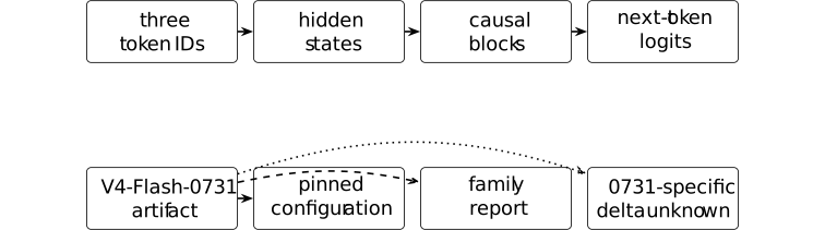
The pinned configuration [⧉] declares 43 layers, hidden width 4096, 64 attention heads, and one key--value head. Section 2 of the family report [⧉] describes the preview architecture. Neither source identifies a complete 0731-specific architecture or training delta. The diagram records the interface, not a small copy of the released model.
5.2. Mechanism families and capability bottlenecks [ftip-00OQ]AGENTDRAFTED
5.2. Mechanism families and capability bottlenecks [ftip-00OQ]AGENTDRAFTED
This map asks which mechanism family changes a declared capability bottleneck and what evidence would show that change. It is a comparison aid, not a ranking of architectures. The shared model, task, intervention, cost and evaluation interfaces remain the conditions of every claim. A source description, a measured result and a transfer claim are kept separate.
The five capability dimensions are state access, the information that can remain available across tokens, steps or external memory operations; adaptive computation, conditional allocation of depth, recurrence, search or stopping together with its charged cost; representation and abstraction, the available representation, composition or predictive state; plasticity, the changes reachable by a declared objective, optimizer, parameter tying and post-training recipe; and portability, survival of a result when the model family, task, scale or deployment regime changes. This is distinct from transfer, which evaluates a frozen artifact on new problems under a common deployment budget. They are coordinates for the capability vector, not a single intelligence scalar.
A bottleneck is the declared resource or interface condition that limits one of these dimensions in a comparison. Cost, numerical stability and monitorability remain evaluation coordinates: the ability to observe the relevant state, compute, update or failure signals under the study protocol. A matched-compute comparison fixes the cost accounting before comparing outcomes; its protocol and the architecture frontier remain authoritative elsewhere in this chapter.
The default core panel contains mechanism families that alter the sequence computation or its state interface. Existing Transformer notation and the decoder-only reference are in § 5.1; the entries below identify the question each family makes testable.
- Transformer reference. Attention exposes token-indexed content access through the declared context and serves as the baseline for the matched-compute comparison and interface comparisons.
- Selective state-space models. The Mamba construction, Sections 3.1--3.3 makes the state-space parameters input-dependent and computes the resulting time-varying recurrence with a hardware-aware scan. The testable bottleneck is how selective compression trades long-context access and throughput against retrieval and portability boundaries; a source mechanism does not settle that tradeoff.
- Linear attention. The linear-attention formulation, Sections 3.2--3.3 uses a feature-map factorization and associative prefix summaries rather than the full softmax attention matrix. The comparison asks which retrieval and memory tasks preserve their evaluation under the changed state interface; it does not identify every hybrid or recurrent model with pure linear attention.
- Internal-tick and looped models. The Continuous Thought Machine, Sections 3.1--3.5 uses a discrete internal tick dimension, private neuron-level models that process activation histories, synchronization as a latent representation, and standard cross-attention to the input features. Its loss selects minimum-loss and maximum-certainty ticks, making variable internal compute a testable mechanism. The looped computations in § 5.3.2 are a separate family; neither is a continuous-time claim, and every extra tick or loop must be charged in the comparison.
- Recurrent or compressed-state mechanisms. The Dragon Hatchling / BDH proposal, Section 3.2 defines a tensor-friendly BDH-GPU state-space system whose attention state admits a reduced representation, alongside local graph dynamics. Its open comparison is whether this state interface supports the target tasks and stable credit assignment at a declared budget; the proposal is not a production result.
The adjunct panel changes an objective, temporal law or function-space bias without being interchangeable with the core architecture families. I-JEPA, Section 3 is an encoder/predictor training architecture as well as an embedding-space prediction objective: its context, target and predictor use ViT backbones, the target encoder is updated by exponential moving average, and masked target blocks are predicted from a context block. That predictive objective leaves a specific representation limit: retaining or recovering the latent state does not by itself identify which directions are invariant and which vary across matched observations. SplitJEPA, Sections 3.1--3.4 (the project overview) makes the boundary explicit—predictive recovery can leave a global orthogonal mixing—and resolves it under stationary Gaussian predictive dynamics, a full-rank second moment of variant differences across invariant correspondences, and representation normalization, by identifying invariant and variant subspaces up to within-block isometries without an observation decoder. Here SplitJEPA is a structured JEPA adjunct and a conditional identifiability result, not a general guarantee for I-JEPA. Liquid time-constant networks, Sections 1--2 supply input-dependent continuous dynamics and a numerical ODE-solver interface; the Neural Operator formulation, Sections 1 and 3 supplies a function-space lens with discretization-invariant operator layers. The Zoology study, Sections 3--5 provides controlled recall analyses of sequence mixers. These sources motivate hypotheses and controls; they do not establish a common capability ordering or make an adjunct a replacement architecture. The JEPA comparability interface specifies fields that must be fixed for a JEPA-like comparison; it is not the source of I-JEPA's architecture. Combining CTM's internal dynamics with I-JEPA's encoder/predictor package is a proposed joint intervention, not an established result, and would require separate attribution of both components.
For each panel row, a study should name the changed state or compute interface, the bottleneck dimension, the task and intervention, the evidence type, and the transport boundary. Existing architecture-indexed ceilings and matched compute, published paired measurements (§ 5.3.7 and § 5.3.8), conditional frontiers (§ 5.3.9) and study design (§ 5.3.10) provide those controls. Blank, incompatible and unmeasured cells remain findings rather than scores to be filled by intuition.
5.3. Architecture-indexed ceilings and matched compute [ftip-00JF]AGENTDRAFTED
5.3. Architecture-indexed ceilings and matched compute [ftip-00JF]AGENTDRAFTED
This optional section refines the architecture-neutral capability framework only when the question names an architecture, optimizer, or systems implementation. The general model/interface formulation remains available when these fields are unnecessary.
Architecture comparisons below are conditional on a declared task family, evaluation law, intervention class, and scalar cost. Toy bounds are finite results under their displayed assumptions and do not transfer to concrete model instances without verified interface, task, and cost assumptions.
5.3.1. Architecture, optimizer, and systems variables [ftip-00JG]AGENTDRAFTED
5.3.1. Architecture, optimizer, and systems variables [ftip-00JG]AGENTDRAFTED
Architecture, optimizer, and systems fields refine the model/interface description. A comparison depends only on the fields named in its assumptions and conclusion.
Definition 5.3.1.1. Optional architecture refinement [ftip-00JH]AGENTDRAFTED
Definition 5.3.1.1. Optional architecture refinement [ftip-00JH]AGENTDRAFTED
Let \(M\) denote an existing model intervention. An architecture refinement is a record \(A=(\mathcal X,\mathcal Y,\operatorname {Map}_A)\) whose map realizes the same declared input and output interface. Forgetting \(A\) returns \(M\); no architecture claim is made when the field is omitted.
Definition 5.3.1.2. Optimizer and systems records [ftip-00JI]AGENTDRAFTED
Definition 5.3.1.2. Optimizer and systems records [ftip-00JI]AGENTDRAFTED
When needed, extend the record by \(O\) for optimizer and state-update rules, and \(S\) for kernels, precision, memory, cache, and scheduling. The triplet \((A,O,S)\) is descriptive; it is not a scalar intelligence score.
Definition 5.3.1.3. Architecture-indexed evaluation functional [ftip-00JJ]AGENTDRAFTED
Definition 5.3.1.3. Architecture-indexed evaluation functional [ftip-00JJ]AGENTDRAFTED
Fix an architecture \(A\), its base artifact, a declared intervention set \(\mathfrak I_A\), and the common evaluation interface of Convention 4.1.1. Each \(\eta \in \mathfrak I_A\) specifies a protocol \(P_{A,\eta }=\operatorname {PostTrain}(A,\eta )\) in that measurable and absolutely integrable evaluation domain, with real performance \(J_{\rm ev}(P_{A,\eta })\). Let \(c_A(\eta )\in [0,+\infty ]\) be its scalar cost under the study's declared accounting rule: a fixed measured cost or an expected nonnegative cost, as specified. For a finite budget \(C\in \mathbb R_{\geq 0}\), define \[ V_A(C)=\sup \left \{ J_{\rm ev}(P_{A,\eta }): \eta \in \mathfrak I_A,\ c_A(\eta )\leq C \right \}\in \overline {\mathbb R}. \] Infinite-cost interventions are infeasible at every such budget.
As in Definition 4.1.10, the empty feasible set has value \(-\infty \); an unbounded-above feasible score set has value \(+\infty \). The value is real exactly when that set is nonempty and bounded above. Increasing \(C\) enlarges the feasible set, so \(V_A\) is nondecreasing. A finite supremum need not be attained by any intervention.
Frontier differences and derivatives are ordinary real operations only where the relevant values are finite, with differentiability additionally required for a derivative. Cost ratios use the domain in Definition 5.3.3.2. The allowed intervention set, evaluation law, and accounting rule are part of the definition, so \(V_A\) is not a universal intelligence function.
Remark 5.3.1.4. Architecture-neutral projection and gradual complexity [ftip-00JK]AGENTDRAFTED
Remark 5.3.1.4. Architecture-neutral projection and gradual complexity [ftip-00JK]AGENTDRAFTED
A statement that depends only on the model/interface map is invariant under changes to architecture \(A\), optimizer \(O\), or systems \(S\) that leave that map fixed. A conclusion about one of those fields instead requires assumptions that distinguish its possible values.
Definition 5.3.1.5. Three ceiling layers [ftip-00JL]AGENTDRAFTED
Definition 5.3.1.5. Three ceiling layers [ftip-00JL]AGENTDRAFTED
For fixed task and evaluation laws, distinguish the representational ceiling of \(A\), the optimizer-reachable ceiling of \((A,O)\), and the systems-feasible frontier of \((A,O,S,C)\). Each layer is conditional on the objects named; none implies that the next layer attains it.
Definition 5.3.1.6. Capability vector and conditional frontier [ftip-00JM]AGENTDRAFTED
Definition 5.3.1.6. Capability vector and conditional frontier [ftip-00JM]AGENTDRAFTED
For an architecture record \(A\), optimizer record \(O\), systems record \(S\), evaluation configuration \(\mathfrak e\) from Definition 3.1.2.1, and declared intervention \(\eta \) at cost cap \(C\), define the capability vector
\[ \mathbf K(A,O,S,\mathfrak e,\eta ,C) =\bigl (K_{\rm state},K_{\rm adapt},K_{\rm repr}, K_{\rm plast},K_{\rm port}\bigr ). \]Its coordinates respectively record state access, adaptive computation, representation and abstraction, plasticity, and portability under the named task, intervention, evaluation law, and cost accounting. A coordinate may be a descriptive field, an estimand, or \(\bot \) when the record is missing, incompatible, or not measured. The tuple is therefore not a common scalar and does not order architectures without a declared comparison rule.
The five coordinates attach to the existing ceiling layers conditionally: representation claims first require a map from \(A\); optimizer-reachable plasticity requires \((A,O)\); state, adaptive computation, and portability claims require the relevant \((A,O,S)\) interface, task family, and deployment regime. A systems-feasible claim also carries \(C\), the cost vector and its declared scalarization. The records in Definition 5.3.1.1, Definition 5.3.1.2, Definition 5.3.1.5, and Definition 3.1.2.1 remain authoritative.
The scalar frontier \(V_A(C)\) of Definition 5.3.1.3 is a projection onto the declared utility \(J_{\rm ev}\) for one architecture and intervention envelope; it is not a capability coordinate. For a fixed evaluation configuration, a vector-valued study may instead retain the conditional set
\[ \mathcal F_{\mathfrak e}(C) =\operatorname {Pareto}\left \{ \bigl (\mathbf K(A,O,S,\mathfrak e,\eta ,C), J_{\rm ev}(P_{A,\eta }),\mathbf c(P_{A,\eta })\bigr ): c_A(\eta )\leq C \right \}, \]where Pareto dominance is declared for the reported coordinates. The set is conditional on the task, intervention class, evaluation law, cost vector, and missingness rule; it is not a universal intelligence frontier.
Matched-compute arms in § 5.3.4 compare entries only after stating which coordinates are held fixed, which are allowed to vary, and how the cost vector is charged. Cost, numerical stability, and monitorability remain evaluation coordinates alongside the vector, so a lower scalar cost or a stable implementation is not silently counted as a capability increase.
5.3.2. Depth reuse and latent recurrence [ftip-00KG]AGENTDRAFTED
5.3.2. Depth reuse and latent recurrence [ftip-00KG]AGENTDRAFTED
Repeated depth, latent feedback, and recirculation change the computation performed at inference. Relative to the fixed reference autoregressive Transformer, their costs include any extra passes, state, and prefill work.
Definition 5.3.2.1. Computation-axis record [ftip-00KH]AGENTDRAFTED
Definition 5.3.2.1. Computation-axis record [ftip-00KH]AGENTDRAFTED
For an architecture record \(A\), distinguish token steps, feed-forward depth passes, recurrent passes, and latent-state updates. Let \(d(A,r)\) be the declared number of depth passes in run \(r\); it is a computation coordinate, not a synonym for parameter count or reasoning quality.
Remark 5.3.2.2. Looped Transformers as a source result [ftip-00KI]AGENTDRAFTED
Remark 5.3.2.2. Looped Transformers as a source result [ftip-00KI]AGENTDRAFTED
Giannou et al. show that a fixed shallow Transformer placed in a loop can execute programmed iterative computations, including conditional branches and in-context algorithms, in Looped Transformers as Programmable Computers[giannou2023looped]. This is a source result under its program, state, and precision assumptions; it is not a universal claim about language-model capability.
Remark 5.3.2.3. Parameter sharing and width tradeoffs [ftip-00KJ]AGENTDRAFTED
Remark 5.3.2.3. Parameter sharing and width tradeoffs [ftip-00KJ]AGENTDRAFTED
Xue et al. report that depth sharing can reduce trainable parameters while limiting modeling capacity, and study width and mixture-of-experts remedies in Go Wider Instead of Deeper[xue2021wider]. The comparison is empirical and task-specific; it does not identify a depth-independent ceiling.
Remark 5.3.2.4. Virtual logical depth and scaling [ftip-00KK]AGENTDRAFTED
Remark 5.3.2.4. Virtual logical depth and scaling [ftip-00KK]AGENTDRAFTED
Zhu et al. vary virtual logical depth by reusing weights and report reasoning gains at nearly fixed parameter count in Beyond Parameters: Exploring Virtual Logic Depth for Scaling Laws[zhu2025virtualdepth]. Their results motivate a depth coordinate in a scaling study, while leaving knowledge capacity, optimization, and transfer dependent on the declared training and evaluation protocol.
Remark 5.3.2.5. Recirculation as an inference intervention [ftip-00KL]AGENTDRAFTED
Remark 5.3.2.5. Recirculation as an inference intervention [ftip-00KL]AGENTDRAFTED
Mozer et al. introduce inference-time recirculation that feeds latent states back through an off-the-shelf model and report task improvements in Recirculation[mozer2026recirculation]. The added serial prefill and adaptive tuning belong in the systems and inference records; the observation is not a proof of a new representational ceiling.
Remark 5.3.2.6. Latent feedback with a preserved Transformer interface [ftip-00KM]AGENTDRAFTED
Remark 5.3.2.6. Latent feedback with a preserved Transformer interface [ftip-00KM]AGENTDRAFTED
Wang et al. widen the feedback channel between decoding steps with latent feedback while retaining a Transformer and language-modeling interface in Full-bandwidth transformer[wang2026fullbandwidth]. Any reported token or accuracy savings are conditional on the scheduled multi-pass training and measured decoding cost.
Remark 5.3.2.7. Latent prediction as a training intervention [ftip-00KN]AGENTDRAFTED
Remark 5.3.2.7. Latent prediction as a training intervention [ftip-00KN]AGENTDRAFTED
Teoh et al. add next-latent prediction to next-token training and report compact predictive states without changing the Transformer interface in Next-Latent Prediction Transformers Learn Compact World Models[teoh2025nextlatent]. This belongs to the training intervention record, not to an architecture-only comparison.
Example 5.3.2.8. Equal parameters do not fix effective depth [ftip-00KO]AGENTDRAFTED
Example 5.3.2.8. Equal parameters do not fix effective depth [ftip-00KO]AGENTDRAFTED
Two runs can share parameter count while using different numbers of recurrent or latent-feedback passes. A matched study must therefore report the computation-axis record and cannot infer an architecture ceiling from parameters alone.
Definition 5.3.2.9. Depth-reuse model-instance record [ftip-00KP]AGENTDRAFTED
Definition 5.3.2.9. Depth-reuse model-instance record [ftip-00KP]AGENTDRAFTED
For a depth-reuse comparison, record shared weights, pass count, stopping rule, recurrent state, training objective, token and pass FLOPs, prefill and decode latency, memory, and evaluation seeds. A pass-count change is an intervention even when the parameter tensor is unchanged.
Example 5.3.2.10. Fixed-recipe depth comparison [ftip-00KQ]AGENTDRAFTED
Example 5.3.2.10. Fixed-recipe depth comparison [ftip-00KQ]AGENTDRAFTED
In a fixed-recipe arm, hold data, optimizer, feedback, stopping rule, and evaluation law fixed while varying only the declared depth-reuse intervention. The resulting difference is an estimand for that recipe, not a best-achievable comparison.
Remark 5.3.2.11. Scaling surfaces rather than a single law [ftip-00KR]AGENTDRAFTED
Remark 5.3.2.11. Scaling surfaces rather than a single law [ftip-00KR]AGENTDRAFTED
A depth-reuse study may fit a surface over parameters, tokens, passes, and cost. The fit is an empirical summary over its measured range; it does not establish an asymptotic law or a universal saturation point.
Remark 5.3.2.12. Architecture and training are separable records [ftip-00KS]AGENTDRAFTED
Remark 5.3.2.12. Architecture and training are separable records [ftip-00KS]AGENTDRAFTED
Weight sharing, latent objectives, and recirculation can alter optimization without changing the declared external interface. The comparison must retain architecture, training intervention, and systems coordinates separately.
Remark 5.3.2.13. Depth reuse across passes, parameters, and tasks [ftip-00KT]AGENTDRAFTED
Remark 5.3.2.13. Depth reuse across passes, parameters, and tasks [ftip-00KT]AGENTDRAFTED
The cited looped, virtual-depth, latent-feedback, and recirculation results do not show that more passes always improve capability, that parameter sharing dominates added parameters, or that inference-time gains transfer to training or to another task family. Each transfer requires a matched model-instance record.
5.3.3. Ceilings, frontiers, and saturation [ftip-00JN]AGENTDRAFTED
5.3.3. Ceilings, frontiers, and saturation [ftip-00JN]AGENTDRAFTED
Definition 5.3.3.1. Fixed-recipe and tuned frontiers [ftip-00JO]AGENTDRAFTED
Definition 5.3.3.1. Fixed-recipe and tuned frontiers [ftip-00JO]AGENTDRAFTED
The fixed-recipe frontier evaluates one common \(\eta \). The equal-tuning frontier permits architecture-specific choices from a predeclared trial set with the same tuning data and budget. The restricted envelope permits a predeclared class of interventions under \(C\). These are distinct estimands.
Definition 5.3.3.2. Iso-quality cost ratio [ftip-00JP]AGENTDRAFTED
Definition 5.3.3.2. Iso-quality cost ratio [ftip-00JP]AGENTDRAFTED
For a finite real target \(q\in \mathbb R\) and the frontier of Definition 5.3.1.3, define the inverse cost \[ C_A(q)=\inf \{C\in \mathbb R_{\geq 0}:V_A(C)\geq q\} \in [0,+\infty ], \qquad \inf \varnothing =+\infty . \] The iso-quality ratio is defined only on the domain \[ \rho _{A/B}(q)=\frac {C_A(q)}{C_B(q)}, \qquad 0\leq C_A(q)<+\infty , \quad 0<C_B(q)<+\infty . \] The architectures must use the same target, evaluation interface, cost units, and comparison arm. The ratio compares efficiency under these choices.
An inverse cost is a threshold infimum, not an executable minimum. The infimum over budgets may be unattained; even if a budget satisfies \(V_A(C)\geq q\), its performance supremum may be unattained at \(q\). An actual target-achieving intervention requires a separate witness.
Positive individual costs do not guarantee a positive inverse cost. For interventions \(\eta _n\), \(n\geq 1\), with score \(1\) and cost \(1/n\), the target \(q=1\) has \(C_A(1)=0\), although every intervention costs more than zero. If both architectures have this family, the putative ratio is \(0/0\) and is excluded by the displayed domain.
Definition 5.3.3.3. Operational cost vector and scalarization [ftip-00JQ]AGENTDRAFTED
Definition 5.3.3.3. Operational cost vector and scalarization [ftip-00JQ]AGENTDRAFTED
Record training FLOPs, inference FLOPs, wall time, memory, energy, and hardware separately as \(\mathbf c\). A scalar cost \(C=w\cdot \mathbf c\) is a declared study choice with nonnegative units \(w\); changing \(w\) changes the frontier and must not be hidden as architecture quality.
Theorem 5.3.3.4. Finite-window representational obstruction [ftip-00JR]AGENTDRAFTED
Theorem 5.3.3.4. Finite-window representational obstruction [ftip-00JR]AGENTDRAFTED
Consider a causal system whose state after each prefix has at most \(K\) distinct values, and a task with \(K+1\) prefixes requiring pairwise distinct continuation labels. By the pigeonhole principle two prefixes share a state, so at least one continuation label is wrong. This is a finite toy obstruction only; it does not bound a concrete Transformer or KDA instance without a proved reduction to this state model.
Theorem 5.3.3.5. A conditional saturation certificate [ftip-00JS]AGENTDRAFTED
Theorem 5.3.3.5. A conditional saturation certificate [ftip-00JS]AGENTDRAFTED
Let \(V_A\) be the nondecreasing frontier of Definition 5.3.1.3, bounded above by a finite \(U\in \mathbb R\). If an intervention reaches a real target \(q<U\) at a finite cost \(C_q\geq 0\), then at every finite \(C\geq C_q\), \(q\leq V_A(C)\leq U\). In particular \(V_A(C)\) is real and \(0\leq U-V_A(C)\leq U-q\). This elementary certificate is conditional on the bound \(U\); it does not assert that real intelligence saturates.
Example 5.3.3.6. Equal scalar cost does not identify architecture [ftip-00JT]AGENTDRAFTED
Example 5.3.3.6. Equal scalar cost does not identify architecture [ftip-00JT]AGENTDRAFTED
Two systems can have the same scalar \(C\) while differing in memory, latency, and training allocation. A cost-weight change can reverse their ordering without changing either system. Thus a one-factor comparison needs a fixed scalarization and a reported cost vector; no architecture effect follows from equal \(C\) alone.
5.3.4. Matched-compute comparison protocol [ftip-00JU]AGENTDRAFTED
5.3.4. Matched-compute comparison protocol [ftip-00JU]AGENTDRAFTED
Definition 5.3.4.1. Common-recipe comparison arm [ftip-00JV]AGENTDRAFTED
Definition 5.3.4.1. Common-recipe comparison arm [ftip-00JV]AGENTDRAFTED
A common-recipe arm fixes training data, optimizer family, schedule, post-training procedure and feedback, training and post-training budgets, inference budget, and evaluation protocol and draws. Interface-compatible parameter choices are declared in advance as part of each permitted architecture package. The comparison varies that package under the common recipe; any further deviation is recorded as a separate comparison coordinate. Its score difference measures performance under this recipe, not the best attainable result for either architecture.
Definition 5.3.4.2. Equal-tuning-budget comparison arm [ftip-00JW]AGENTDRAFTED
Definition 5.3.4.2. Equal-tuning-budget comparison arm [ftip-00JW]AGENTDRAFTED
An equal-tuning-budget arm permits architecture-specific tuning under a predeclared protocol that fixes the tuning data and its volume, trial count, selection rule, stopping rule, and tuning cost for both architectures. The cost uses the same declared accounting rule. The resulting comparison measures practical performance under this equal optimization effort; it does not determine best possible training or a representation-only limit.
Definition 5.3.4.3. Restricted-envelope comparison arm [ftip-00JX]AGENTDRAFTED
Definition 5.3.4.3. Restricted-envelope comparison arm [ftip-00JX]AGENTDRAFTED
A restricted-envelope arm declares an allowed intervention class \(\mathcal E_A\subseteq \mathfrak I_A\) for each architecture, specifying the permitted training, post-training, and inference procedures. The classes expose exclusions, search budgets, seeds, and stopping rules. Restrict the evaluation functional of Definition 5.3.1.3 to \(\mathcal E_A\) and compare the resulting suprema under the same finite cost cap \(C\geq 0\), common evaluation law, and common declared cost accounting.
The measurable, integrable evaluation domain and extended-real conventions of Definition 5.3.1.3 apply: an empty feasible class has value \(-\infty \), an unbounded-above feasible score set has value \(+\infty \), and a finite supremum need not be attained. The allowed class is part of the comparison, so its envelope is a restriction-dependent quantity, not an unrestricted architectural ceiling.
Definition 5.3.4.4. Model-instance comparison evidence record [ftip-00JY]AGENTDRAFTED
Definition 5.3.4.4. Model-instance comparison evidence record [ftip-00JY]AGENTDRAFTED
A model-instance record contains architecture/checkpoint identity, parameter count, data and post-training recipe, optimizer, precision, hardware, cache policy, training and inference cost vectors, task suite, and independent evaluation seed. A missing field makes an architecture attribution unknown.
Remark 5.3.4.5. Systems optimizations are measured interventions [ftip-00JZ]AGENTDRAFTED
Remark 5.3.4.5. Systems optimizations are measured interventions [ftip-00JZ]AGENTDRAFTED
FlashAttention, KV-cache layouts, quantization, batching, and kernels can change feasible cost. If they approximate, truncate, or alter precision of the mathematical computation, the record must mark that as a systems intervention rather than as a pure architecture comparison.
Theorem 5.3.4.6. Matched-protocol difference is an estimand [ftip-00K0]AGENTDRAFTED
Theorem 5.3.4.6. Matched-protocol difference is an estimand [ftip-00K0]AGENTDRAFTED
Given \(n\geq 1\) evaluation draws, let \(\widehat V_A(C)\) be the sample mean of finite real evaluation scores for architecture \(A\) at a finite cost cap \(C\geq 0\). Under a fixed evaluation law and common-recipe arm, the finite difference \(\widehat V_A(C)-\widehat V_B(C)\) is a well-defined empirical estimand.
It does not identify a causal architecture effect when data, tuning, or systems coordinates differ. The conclusion follows directly from the declared record.
Remark 5.3.4.7. Conditions for applying a toy model [ftip-00K1]AGENTDRAFTED
Remark 5.3.4.7. Conditions for applying a toy model [ftip-00K1]AGENTDRAFTED
A toy theorem applies to a concrete model only if an explicit map from its state and interface to the model preserves the theorem's assumptions, including its cost accounting. Without such a map, the conclusion concerns only the abstract model; its validity for the concrete system is unknown.
5.3.5. Kimi Delta Attention versus Transformer [ftip-00K2]AGENTDRAFTED
5.3.5. Kimi Delta Attention versus Transformer [ftip-00K2]AGENTDRAFTED
Definition 5.3.5.1. KDA model-instance record [ftip-00K3]AGENTDRAFTED
Definition 5.3.5.1. KDA model-instance record [ftip-00K3]AGENTDRAFTED
For a Kimi Delta Attention (KDA) versus full-attention baseline study, record the exact Kimi Linear checkpoint, layer mix, context length, hardware, kernel, precision, batch, and decoding workload. The paper describes KDA as a fine-grained gated delta-rule module in a hybrid architecture; those are source observations from Kimi Linear: An Expressive, Efficient Attention Architecture[kimi2025linear], not universal theorems.
If the baseline is called a Transformer, record whether it is the paper's MLA baseline or another full-attention implementation; the label alone does not identify a common architecture or cost.
Example 5.3.5.2. Matched-cost KDA and Transformer comparison [ftip-00K4]AGENTDRAFTED
Example 5.3.5.2. Matched-cost KDA and Transformer comparison [ftip-00K4]AGENTDRAFTED
A matched comparison uses the same task prompts, post-training data and feedback, optimizer family, evaluation protocol, and quality target. The corresponding measurements include parameter count, training FLOPs, inference FLOPs, wall time, memory, KV-cache bytes, and context length for each architecture. A reported speed or quality difference is conditional on these experimental conditions and measurements.
Remark 5.3.5.3. What the Kimi Linear paper establishes [ftip-00K5]AGENTDRAFTED
Remark 5.3.5.3. What the Kimi Linear paper establishes [ftip-00K5]AGENTDRAFTED
Kimi Linear reports a hybrid KDA/MLA model and fair-comparison experiments in Sections 3--5, with setup in Section 5.4 and efficiency comparisons in Sections 5.5--5.6 of Kimi Linear: An Expressive, Efficient Attention Architecture[kimi2025linear]. These include long-context efficiency.
The reported throughput and quality are empirical under its training recipe and hardware; they are lower bounds on demonstrated performance, not an architecture-independent ceiling.
Example 5.3.5.4. Parameter matching is not cost matching [ftip-00K6]AGENTDRAFTED
Example 5.3.5.4. Parameter matching is not cost matching [ftip-00K6]AGENTDRAFTED
Two models with equal parameter count can have different attention FLOPs, KV-cache memory, kernel utilization, and attainable context. Conversely, equal wall time can hide different hardware and precision. Therefore a parameter-matched result cannot by itself identify a compute frontier.
Remark 5.3.5.5. Cache, throughput, and quality in KDA comparisons [ftip-00K7]AGENTDRAFTED
Remark 5.3.5.5. Cache, throughput, and quality in KDA comparisons [ftip-00K7]AGENTDRAFTED
The KDA example does not prove that every linear-attention model beats every Transformer, that cache savings imply equal quality, or that a measured throughput gain is a capability gain. Any such statement requires a new matched study with the evidence record of Definition 5.3.4.4.
Definition 5.3.5.6. Model-instance comparison decision rule [ftip-00K8]AGENTDRAFTED
Definition 5.3.5.6. Model-instance comparison decision rule [ftip-00K8]AGENTDRAFTED
Call architecture A more cost-efficient than B at quality \(q\) only when the compared threshold costs use the same declared protocol, the confidence procedure and stopping rule are fixed, and all cost-vector coordinates needed by the claim are present. A ratio additionally requires finite costs and a strictly positive denominator as in Definition 5.3.3.2. State whether the costs are measured target-achieving witnesses or justified inverse-frontier values \(C_A(q)\) and \(C_B(q)\); observing one successful run does not identify those infima. Otherwise the comparison is descriptive or unknown.
5.3.6. Interface boundaries for alternative architectures [ftip-00K9]AGENTDRAFTED
5.3.6. Interface boundaries for alternative architectures [ftip-00K9]AGENTDRAFTED
Definition 5.3.6.1. JEPA comparability interface [ftip-00KA]AGENTDRAFTED
Definition 5.3.6.1. JEPA comparability interface [ftip-00KA]AGENTDRAFTED
A JEPA-like architecture is comparable to an autoregressive model only after fixing the predictor, target representation, decoder or downstream interface, training objective, inference procedure, and evaluation law. A parameter-count match alone is not a typed comparison.
Remark 5.3.6.2. Representation and task interface are separate [ftip-00KB]AGENTDRAFTED
Remark 5.3.6.2. Representation and task interface are separate [ftip-00KB]AGENTDRAFTED
A latent predictor can be excellent under one decoder and unusable under another. The evaluation record must therefore include the interface that maps the representation to the declared task output.
Theorem 5.3.6.3. Interface-preserving architecture reduction [ftip-00KC]AGENTDRAFTED
Theorem 5.3.6.3. Interface-preserving architecture reduction [ftip-00KC]AGENTDRAFTED
If two architecture records induce the same conditional output law on a fixed task and evaluation interface, every evaluation functional \(J\) gives the same value. This is an immediate pushforward identity under the stated output-law and interface assumptions. It does not imply that distinct architectures are generally equivalent.
Example 5.3.6.4. Equal benchmark score can hide different ceilings [ftip-00KD]AGENTDRAFTED
Example 5.3.6.4. Equal benchmark score can hide different ceilings [ftip-00KD]AGENTDRAFTED
Two architectures may tie on a finite benchmark while differing on an unmeasured task slice or longer context. Thus a single score cannot establish equal representational ceilings; the task family and evaluation coverage must be declared.
Remark 5.3.6.5. Architecture-independent model interfaces [ftip-00KE]AGENTDRAFTED
Remark 5.3.6.5. Architecture-independent model interfaces [ftip-00KE]AGENTDRAFTED
A result stated solely in terms of a model/interface map applies to every architecture realizing that map and satisfying its hypotheses. An architecture-specific conclusion can require further assumptions, as in Remark 5.3.1.4.
Remark 5.3.6.6. Open model-instance questions [ftip-00KF]AGENTDRAFTED
Remark 5.3.6.6. Open model-instance questions [ftip-00KF]AGENTDRAFTED
The relative capability and cost of KDA, full attention, and JEPA candidates remain empirical questions. A reproducible comparison requires identified checkpoints or reproducible training, fixed evaluation seeds, and measured cost vectors. Architecture-specific ceilings remain estimands and hypotheses rather than established constants.
5.3.7. Published hybrid-attention comparison [ftip-00KU]AGENTDRAFTED
5.3.7. Published hybrid-attention comparison [ftip-00KU]AGENTDRAFTED
Kimi Linear combines recurrent KDA layers with periodic full MLA attention. Its published comparison shows task-dependent score changes and lower long-context decoding times. The selected scores in Example 5.3.8.8, the memory estimate in Example 5.3.7.4, and the discovery calculation in Example 5.3.7.9 connect these observations to a post-training question: when can a cheaper attempt compensate for a possible lower per-attempt success probability?
Example 5.3.7.1. Published Kimi Linear operating point [ftip-00KV]AGENTDRAFTED
Example 5.3.7.1. Published Kimi Linear operating point [ftip-00KV]AGENTDRAFTED
The Kimi Linear report compares experimental models pretrained on 1.4 trillion tokens, each with 48 billion total and 3 billion active parameters. Kimi Linear uses three Kimi Delta Attention layers for each full Multi-head Latent Attention layer, with no positional encoding (NoPE) in its MLA layers; the reference uses full MLA attention [kimi2025linear, Sections 4 and 5.4]. These are properties of the reported hybrid architecture.
These experimental models are distinct from the released Kimi Linear model, pretrained on 5.7 trillion tokens and supporting up to one million tokens of context. Appendix D compares that release with Moonlight, which has 16 billion total and 3 billion active parameters [kimi2025linear, Section 5.4.1 and Appendix D].
Example 5.3.7.2. Published efficiency observations [ftip-00KW]AGENTDRAFTED
Example 5.3.7.2. Published efficiency observations [ftip-00KW]AGENTDRAFTED
For batch size one at one million tokens, Figure 7 labels a \(2.9\times \) prefill speedup and a \(2.2\times \) decoding speedup for Kimi Linear against MLA. Section 6.3 gives \(2.3\times \) for the latter point, so the graphic and prose differ slightly [kimi2025linear, Figure 7 and Sections 5.6 and 6.3].
The larger-batch comparison in Figure 1(b) gives decoding time per output token of 1.84 milliseconds for Kimi Linear and 11.48 milliseconds for MLA, with a reported \(6.3\times \) speedup. Section 6.3 describes this as a theoretical speedup from reallocating saved KV-cache memory to larger batches. It illustrates a different use of the memory saving from the batch-one latency result [kimi2025linear, Figure 1(b) and Section 6.3].
Figure 1(a) reports RULER scores of 84.3 for Kimi Linear and 81.3 for MLA at 128k context, with \(3.98\times \) decoding acceleration [kimi2025linear, Figure 1(a)]. The report also gives a reduction of up to 75 percent in KV-cache use [kimi2025linear, Abstract]. Together these observations motivate studying context length and batch size as separate cost coordinates. The unequal RULER scores and different timing regimes are retained when interpreting those points.
Definition 5.3.7.3. Quality target and cost measurement [ftip-00KX]AGENTDRAFTED
Definition 5.3.7.3. Quality target and cost measurement [ftip-00KX]AGENTDRAFTED
For a reported benchmark score q, use the same task, prompt law, scoring rule, and post-training condition for both systems. The comparison records the smallest measured cost at which each system reaches q, when such a measurement exists. A throughput or cache ratio is not substituted for this iso-quality cost.
Example 5.3.7.4. A cache-memory estimate for hybrid attention [ftip-00KY]AGENTDRAFTED
Example 5.3.7.4. A cache-memory estimate for hybrid attention [ftip-00KY]AGENTDRAFTED
The cited FLA KDA implementation at commit 6b6f546f stores one active recurrent state
per sequence, with dimensions determined by the value heads and key/value
dimensions rather than accumulated context length. Its newly allocated
state uses float32
[⧉].
The optional short-convolution state has one fixed-width kernel buffer per
channel and sequence
[⧉].
This supplies a concrete implementation model for the recurrent part of
the 3:1 mixture in Example 5.3.7.1.
Consider a stylized comparison with \(4\ell \) layers, batch size \(b\), and context length \(T\), where \(\ell ,b,T\) are positive integers. Assume each MLA layer stores \(\kappa T\) bytes per sequence, with the same \(\kappa >0\) in both designs, and each KDA layer stores one terminal recurrent-plus-convolution state of \(\sigma >0\) bytes. The active attention-state memories are
\[ M_{\rm MLA}=4b\ell \kappa T,\qquad M_{\rm hybrid}=b\ell (\kappa T+3\sigma ),\qquad \frac {M_{\rm hybrid}}{M_{\rm MLA}} =\frac {1}{4}+\frac {3\sigma }{4\kappa T}. \]The hybrid uses less active state exactly when \(T>\frac {\sigma }{\kappa }\), and the ratio tends to \(1/4\) as context grows. This explains why replacing three quarters of the growing caches can approach a 75-percent saving, while fixed recurrent-state overhead can erase the advantage at short contexts. The retained MLA layers keep the hybrid's state memory linear in \(T\); the whole model is not a fixed-memory recurrent system.
Weights, training activations, workspaces, allocator padding and saved prefix states are outside this active-state calculation. At a fixed device memory budget, the estimate predicts more room for simultaneous or longer rollouts when attention state dominates. It does not predict a fourfold speedup. Training and decoding also use different execution paths: FLA selects chunk kernels for gradient-enabled computation and fused recurrence for short inference calls [⧉]. The fixed-state estimate is therefore a useful serving hypothesis, not a training-memory or training-speed formula.
Example 5.3.7.5. Common-recipe reading of the Kimi result [ftip-00KZ]AGENTDRAFTED
Example 5.3.7.5. Common-recipe reading of the Kimi result [ftip-00KZ]AGENTDRAFTED
The report holds its stated pretraining and SFT recipes common across the experimental models [kimi2025linear, Sections 5.4--5.5 and Table 4]. The selected observations in Example 5.3.8.8 compare the resulting trained designs, including the hybrid's 3:1 KDA/MLA pattern and NoPE choice. The mixed score directions suggest a task-dependent tradeoff rather than one ordering of the two architectures.
The theoretical mechanism is a change in the cost of maintaining and using the prefix: recurrent layers compress it into state, while the retained MLA layers preserve growing attention caches. The model in Example 5.3.7.4 predicts the largest memory advantage at long contexts. If this advantage reduces the cost of generating useful candidates, Example 5.3.7.9 predicts when more attempts can offset a reduction in per-attempt quality. This is a conditional explanation to test through rollout costs and verified success rates; it does not require attributing the whole result to KDA alone.
Example 5.3.7.6. Measured iso-quality cost ratio [ftip-00L0]AGENTDRAFTED
Example 5.3.7.6. Measured iso-quality cost ratio [ftip-00L0]AGENTDRAFTED
Let \(c_K(q)\) and \(c_T(q)\) be measured inference costs for Kimi Linear and the Transformer reference at the same finite real score \(q\) and context length, under one accounting rule. If \(0\leq c_K(q)<+\infty \) and \(0<c_T(q)<+\infty \), the measured ratio \(\widehat \rho _{K/T}(q)=c_K(q)/c_T(q)\) is reported together with the full cost vectors. These measured costs need not be the inverse frontier infima of Definition 5.3.3.2. If either threshold is unmeasured or the denominator is zero, the ratio is left undefined rather than inferred from the paper's speedup plot.
Remark 5.3.7.7. Hybrid attention is not pure linear attention [ftip-00L1]AGENTDRAFTED
Remark 5.3.7.7. Hybrid attention is not pure linear attention [ftip-00L1]AGENTDRAFTED
Kimi Linear combines KDA with periodic full-attention layers. A measured advantage therefore identifies the reported hybrid intervention, not a claim that a purely linear recurrent architecture has the same quality or ceiling. The layer pattern belongs in the architecture record.
Remark 5.3.7.8. Demonstrated performance is a lower bound [ftip-00L2]AGENTDRAFTED
Remark 5.3.7.8. Demonstrated performance is a lower bound [ftip-00L2]AGENTDRAFTED
The published benchmark scores demonstrate attainable points for the reported checkpoints and protocol. They do not establish a representational ceiling, a universal scaling law, or a claim that additional cost cannot improve either architecture.
Example 5.3.7.9. When cheaper attempts compensate for lower success [ftip-00L3]AGENTDRAFTED
Example 5.3.7.9. When cheaper attempts compensate for lower success [ftip-00L3]AGENTDRAFTED
Smaller caches can support more concurrent requests or avoid preemption and recomputation. These are actual serving mechanisms in vLLM's memory and scheduling guidance [⧉]. For post-training, the useful prediction is therefore about completed candidate attempts under a budget, including verification and optimization costs, rather than decoding speed alone.
Use the following cost model on the same hardware. One baseline attempt costs \(c>0\); generation accounts for a fraction \(f\in [0,1]\). Suppose generation becomes \(s_{\rm gen}>0\) times as fast while all other cost per attempt stays fixed. The new cost and total attempt-throughput factor are
\[ c_K=c\left (1-f+\frac {f}{s_{\rm gen}}\right ),\qquad S=\frac {c}{c_K} =\frac {1}{1-f+f/s_{\rm gen}}. \]For a fixed budget \(B\geq 0\), this model permits \(N_M=\lfloor B/c\rfloor \) baseline attempts and \(N_K=\lfloor B/c_K\rfloor \) hybrid attempts. Assume \(N_M,N_K\geq 1\) and verified-success events independent within each set of attempts, with respective probabilities \(p_M,p_K\in [0,1]\). Then Theorem 4.4.1.2 gives discovery probabilities \(1-(1-p_M)^{N_M}\) and \(1-(1-p_K)^{N_K}\). The hybrid matches or exceeds baseline discovery exactly when
\[ p_K\geq 1-(1-p_M)^{N_M/N_K}. \]This follows by comparing the two failure probabilities and taking the nonnegative \(N_K\)-th root.
For an illustrative estimate, suppose generation consumes 80 percent of the baseline cost and use \(s_{\rm gen}=2.2\), motivated by the batch-one decode figure in Example 5.3.7.2. Applying that decode factor to the whole generation stage is a working approximation, not a measured rollout result. Then \(S\approx 1.774\); a budget of \(B=10c\) buys 10 baseline attempts or 17 hybrid attempts. If \(p_M=0.10\) and \(p_K=0.08\), the discovery probabilities are approximately \(0.651\) and \(0.758\). The break-even hybrid probability is about \(0.0601\). Thus this model predicts that more attempts can outweigh a moderate per-attempt quality loss. The assumed probabilities are illustrative verified-success rates, not conversions of the benchmark scores in Example 5.3.8.8.
The prediction is strongest for long-context, generation-heavy work whose saved memory becomes usable rollout capacity. As verification or optimization dominates, \(f\) shrinks and \(S\) approaches one. Correlated attempts require the joint-law analysis of Convention 4.4.1.1 instead of the independent product. Measure completed attempts, verified-success rates and total cost under a fixed prompt, decoding and verifier protocol to test the tradeoff. In the RLVR round of Example 2.9.20, additional successful candidates can improve the available feedback; whether they produce useful accepted updates is a further optimizer-and-evaluation question, as Example 4.4.4.7 demonstrates.
5.3.8. Paired measurements for model comparison [ftip-00L4]AGENTDRAFTED
5.3.8. Paired measurements for model comparison [ftip-00L4]AGENTDRAFTED
A paired measurement specifies both model instances and their task, intervention, evaluation, and cost coordinates. These conditions determine the meaning of each point in the measured frontier.
Definition 5.3.8.1. Comparison pair identity [ftip-00L5]AGENTDRAFTED
Definition 5.3.8.1. Comparison pair identity [ftip-00L5]AGENTDRAFTED
A paired comparison identifies the two systems, exact checkpoint or training commit, architecture variant, parameter counts, tokenizer, and context limit. A label such as ``Transformer'' is insufficient when attention, cache, or layer patterns differ.
Definition 5.3.8.2. Common task and evaluation conditions [ftip-00L6]AGENTDRAFTED
Definition 5.3.8.2. Common task and evaluation conditions [ftip-00L6]AGENTDRAFTED
Both systems use the same task family, prompt and data law, scoring rule, sampling seeds, stopping rule, and evaluator version. Any exception is a separate comparison arm, not an unrecorded architecture effect.
Definition 5.3.8.3. Training and post-training coordinates [ftip-00L7]AGENTDRAFTED
Definition 5.3.8.3. Training and post-training coordinates [ftip-00L7]AGENTDRAFTED
Record data volume, token order policy, optimizer and schedule, supervised tuning, feedback or reinforcement procedure, update count, and selection rule. The common-recipe arm fixes these coordinates; the equal-tuning arm allows predeclared alternatives with equal search resources.
Definition 5.3.8.4. Inference and systems coordinates [ftip-00L8]AGENTDRAFTED
Definition 5.3.8.4. Inference and systems coordinates [ftip-00L8]AGENTDRAFTED
Record hardware, software and kernel versions, precision, batch, cache policy, sequence lengths, warm-up procedure, concurrency, and decoding settings. A kernel or cache change that alters numerical computation is marked as an intervention rather than hidden as an implementation detail.
Definition 5.3.8.5. Per-system cost vector [ftip-00L9]AGENTDRAFTED
Definition 5.3.8.5. Per-system cost vector [ftip-00L9]AGENTDRAFTED
For each system, the cost vector \(\mathbf c\) contains training FLOPs, inference FLOPs, wall time, memory, energy when available, and context length. The primary scalar \(C\) and its weights are declared beside the vector; omitted coordinates are marked unknown.
Definition 5.3.8.6. Repeated measurement rule [ftip-00LA]AGENTDRAFTED
Definition 5.3.8.6. Repeated measurement rule [ftip-00LA]AGENTDRAFTED
For each fixed workload and system, record warm-up runs, repetition count, random seeds, and the aggregation rule. Report mean and dispersion for time, memory, and score; a single fastest run cannot define a cost frontier.
Definition 5.3.8.7. Paired uncertainty estimates [ftip-00LB]AGENTDRAFTED
Definition 5.3.8.7. Paired uncertainty estimates [ftip-00LB]AGENTDRAFTED
When the same evaluation items are used, report paired score differences and an uncertainty procedure fixed before inspecting the result. Confidence intervals quantify sampling variation; they do not repair unmatched training, systems, or task coordinates.
Example 5.3.8.8. Published Kimi Linear comparison [ftip-00LC]AGENTDRAFTED
Example 5.3.8.8. Published Kimi Linear comparison [ftip-00LC]AGENTDRAFTED
Table 4 of the Kimi Linear report compares the experimental models pretrained on 1.4 trillion tokens in Example 5.3.7.1, after the same supervised fine-tuning (SFT) recipe. Both have 48 billion total and 3 billion active parameters. Three selected benchmark scores are [kimi2025linear, Sections 4 and 5.4 and Table 4]:
| Arm | MMLU-Pro | LiveBench | EvalPlus |
|---|---|---|---|
| Kimi Linear | 67.4 | 45.2 | 61.0 |
| Full MLA | 65.7 | 45.7 | 62.6 |
The entries use the paper's score units, with larger values better on each selected benchmark; LiveBench is reported as Pass@1. Kimi Linear is higher on MMLU-Pro and lower on LiveBench and EvalPlus in these observations. These are reported point estimates on different tasks, not a single capability score; the table supplies no uncertainty estimate.
The common recipe uses the K2 pretraining corpus, MuonClip and a shared training schedule. SFT proceeds from broad instruction data to targeted reasoning tasks; evaluation uses temperature 1.0 and an internal framework derived from LM-Harness [kimi2025linear, Section 5.4]. Thus the scores provide a concrete example of how the trained hybrid and full-MLA designs respond to the same recipe. The cost mechanism and its possible post-training consequences are developed in Example 5.3.7.5.
Remark 5.3.8.9. Measured and assumed costs [ftip-00LD]AGENTDRAFTED
Remark 5.3.8.9. Measured and assumed costs [ftip-00LD]AGENTDRAFTED
A useful cost model can combine measurements with assumptions justified by the architecture and its implementation. In Example 5.3.7.9, the generation share \(f\) and speed factor \(s_{\rm gen}\) determine a predicted attempt-throughput factor. Their assumed values can be varied without pretending they were measured in the original experiment.
For fixed \(f\in [0,1]\), write \(S(s)=1/(1-f+f/s)\) for \(s>0\). This function is nondecreasing. An interval \(s_{\rm gen}\in [s_-,s_+]\), with \(0<s_-\leq s_+\), therefore gives the conditional range \(S\in [S(s_-),S(s_+)]\). This is sensitivity to a chosen assumption range; it is a statistical confidence interval only if a sampling argument supplies that interpretation.
Definition 5.3.8.10. Measured contrasts and conditional predictions [ftip-00LE]AGENTDRAFTED
Definition 5.3.8.10. Measured contrasts and conditional predictions [ftip-00LE]AGENTDRAFTED
A measured paired contrast evaluates the same declared quantity for two observed model instances under a specified task, protocol and cost accounting. The common-recipe scores in Example 5.3.8.8 are one example. A confirmatory comparison fixes its matching and selection rules before examining the scores.
A conditional paired prediction instead uses an explicit model to supply one or more cost or response quantities, then derives the comparison under those assumptions. The discovery probabilities in Example 5.3.7.9 are an example. Such a prediction can be motivated by existing observations and guide a later experiment; its unmeasured inputs remain assumptions, and agreement with new matched measurements tests the model.
Example 5.3.8.11. How generation share changes the predicted gain [ftip-00LF]AGENTDRAFTED
Example 5.3.8.11. How generation share changes the predicted gain [ftip-00LF]AGENTDRAFTED
Keep the illustrative generation factor \(s_{\rm gen}=2.2\) from Example 5.3.7.9 and vary the baseline generation share \(f\). Its cost model gives the following total attempt-throughput factors:
| Generation share | Predicted throughput factor |
|---|---|
| 20 percent | 1.122 |
| 50 percent | 1.375 |
| 80 percent | 1.774 |
| 100 percent | 2.200 |
These calculated values show why the same decoding improvement can matter much more for generation-heavy search than for a verifier- or optimizer-dominated workload. They suggest measuring the time spent in generation, verification and updates before selecting where to invest systems effort. A change in the bottleneck changes the useful intervention, even when the attention architecture stays fixed.
Remark 5.3.8.12. Testing the predicted architecture tradeoff [ftip-00LG]AGENTDRAFTED
Remark 5.3.8.12. Testing the predicted architecture tradeoff [ftip-00LG]AGENTDRAFTED
The memory and discovery models predict the strongest benefit when long prefixes make attention state expensive, saved capacity improves useful rollout throughput, and per-attempt success remains above the break-even threshold. Short contexts, expensive verification, or strongly correlated attempts can weaken that benefit. These are distinct mechanisms to test, rather than a universal ranking of KDA and full attention.
A comparison across implementations can retain this reasoning while re-estimating state sizes, generation share and success probabilities for the new system. Report both the prediction and the matched measurements: their agreement or disagreement identifies which mechanism or assumption needs revision.
5.3.9. Conditional frontier and saturation analysis [ftip-00LH]AGENTDRAFTED
5.3.9. Conditional frontier and saturation analysis [ftip-00LH]AGENTDRAFTED
A finite matched study measures capability at selected values of one declared cost. Its frontier and saturation target are conditional on that protocol; they do not establish a universal intelligence law.
Definition 5.3.9.1. Finite cost grid [ftip-00LI]AGENTDRAFTED
Definition 5.3.9.1. Finite cost grid [ftip-00LI]AGENTDRAFTED
Choose a finite ordered grid \(0<C_1<\cdots <C_m\) and evaluate each architecture at every declared grid point under the same task and protocol. The resulting values \(\widehat V_A(C_i)\) are observations of the restricted frontier, not its values between grid points.
Definition 5.3.9.2. Observed upper envelope [ftip-00LJ]AGENTDRAFTED
Definition 5.3.9.2. Observed upper envelope [ftip-00LJ]AGENTDRAFTED
For an observed score \(s_A(C_i)\) define the discrete upper envelope \(U_A(C_i)=\max _{j\leq i}s_A(C_j)\). It is a descriptive monotone summary of the measured points; it is not evidence that unmeasured costs attain the envelope or that extra cost cannot reduce score.
Definition 5.3.9.3. Uncertainty bands on the frontier [ftip-00LK]AGENTDRAFTED
Definition 5.3.9.3. Uncertainty bands on the frontier [ftip-00LK]AGENTDRAFTED
Attach a predeclared uncertainty interval \(I_A(C_i)\) to each score and carry those intervals through score differences and threshold crossings. A finite band describes sampling and measurement variation; it does not cover unmeasured training procedures or architectures.
Definition 5.3.9.4. Declared saturation target [ftip-00LL]AGENTDRAFTED
Definition 5.3.9.4. Declared saturation target [ftip-00LL]AGENTDRAFTED
Fix a quality target \(q\in \mathbb R\), tolerance and cost increment \(\varepsilon ,\delta \in (0,+\infty )\), and a budget \(C\in \mathbb R_{\geq 0}\). Require both \(V_A(C)\) and \(V_A(C+\delta )\) to be finite real values. A study calls an architecture \(\varepsilon \)-saturated at \(C\) only relative to its allowed intervention class when the restricted frontier has certified gain \(V_A(C+\delta )-V_A(C)\leq \varepsilon \).
Theorem 5.3.9.5. Conditional saturation certificate [ftip-00LM]AGENTDRAFTED
Theorem 5.3.9.5. Conditional saturation certificate [ftip-00LM]AGENTDRAFTED
Take finite real \(U\), \(C\geq 0\), \(\delta \geq 0\), and \(\varepsilon \geq 0\), with the nondecreasing frontier of Definition 5.3.1.3. If a justified upper bound gives \(V_A(C+\delta )\leq U\) and a justified lower bound gives \(V_A(C)\geq U-\varepsilon \), then \(U-\varepsilon \leq V_A(C)\leq V_A(C+\delta )\leq U\). Both endpoint values are therefore finite real, and \(0\leq V_A(C+\delta )-V_A(C)\leq \varepsilon \). This is a conditional bound for the named frontier; it proves no universal saturation of intelligence.
For the finite controller class with hard resource admission, Corollary 3.1.5.2.4 obtains the required bounds from a feasible controller and a uniform Bellman certificate.
Example 5.3.9.6. Finite observations need not identify a frontier [ftip-00LN]AGENTDRAFTED
Example 5.3.9.6. Finite observations need not identify a frontier [ftip-00LN]AGENTDRAFTED
Let \(S\subset \mathbb R_{\geq 0}\) be a finite set of measured costs, and choose \(C_0>0\) larger than every element of \(S\). Suppose the exact frontier value observed at each cost in \(S\) is zero. For finite budgets \(C\geq 0\), suppose the declared class of possible frontiers permits both \[ V_0(C)=0, \qquad V_1(C)= \begin {cases} 0,&0\leq C<C_0,\\ 1,&C\geq C_0. \end {cases} \] These nondecreasing frontiers with scores in \([0,1]\) agree on every observed cost and differ at \(C_0\). The observations alone do not distinguish them.
Both possibilities have finite realizations in the framework of Definition 5.3.1.3: allow two interventions with costs \(0\) and \(C_0\). Give the first score zero and the second score \(\theta \in \{0,1\}\). For example, on a single deterministic evaluation task with utility equal to the output bit, let the two resulting protocols return \(0\) and \(\theta \). The two possible choices of \(\theta \) give \(V_0\) and \(V_1\), respectively, under the same intervention and cost specification. Every score is finite, and the feasible score maximum is attained at each budget.
This example does not supply a strictly better agreeing frontier for every possible data set or every admissible class. If a proved global score bound is \(1\) and an intervention attains it at a finite cost \(C_*\geq 0\), monotonicity forces \(V_A(C)=1\) for every \(C\geq C_*\); no higher value is admissible. A singleton class of possible frontiers can also identify the frontier without such an alternative. A conditional certificate such as Theorem 5.3.9.5 therefore requires its stated upper-bound evidence; that evidence does not follow merely from the absence of an observed improvement.
Definition 5.3.9.7. One-factor cost interpretation [ftip-00LO]AGENTDRAFTED
Definition 5.3.9.7. One-factor cost interpretation [ftip-00LO]AGENTDRAFTED
The primary cost \(C\) is a declared scalarization of the recorded cost vector. A frontier statement is conditional on its units and weights; the same paired measurements may produce a different ordering under a different scalarization.
Example 5.3.9.8. Crossing architecture frontiers [ftip-00LP]AGENTDRAFTED
Example 5.3.9.8. Crossing architecture frontiers [ftip-00LP]AGENTDRAFTED
Two architectures may alternate in the observed ordering across costs: one can score higher at small \(C\) while the other catches up at larger \(C\). Thus a single comparison point cannot establish a global ordering or a common ceiling.
Example 5.3.9.9. Frontier report for the KDA study [ftip-00LQ]AGENTDRAFTED
Example 5.3.9.9. Frontier report for the KDA study [ftip-00LQ]AGENTDRAFTED
A Kimi Delta Attention versus Transformer study should publish the cost grid, paired scores, uncertainty intervals, scalarization weights, and the exact identities and configurations of the compared models. The report may then state which measured points are Pareto or iso-quality comparisons under that protocol.
Remark 5.3.9.10. Frontiers depend on the intervention and evaluation [ftip-00LR]AGENTDRAFTED
Remark 5.3.9.10. Frontiers depend on the intervention and evaluation [ftip-00LR]AGENTDRAFTED
The conditional frontier is indexed by architecture, intervention class, task family, evaluation law, and cost scalarization. Changing any of these coordinates creates a new estimand; no ordering transfers automatically to a new checkpoint, optimizer, hardware stack, or task family.
5.3.10. Study design for comparisons across model instances [ftip-00LS]AGENTDRAFTED
5.3.10. Study design for comparisons across model instances [ftip-00LS]AGENTDRAFTED
This subsection specifies how a conditional architecture comparison may be instantiated without changing the architecture-neutral formulation. It is a study design, not a universal ranking of architectures.
Definition 5.3.10.1. Matched model-instance record [ftip-00LT]AGENTDRAFTED
Definition 5.3.10.1. Matched model-instance record [ftip-00LT]AGENTDRAFTED
A model-instance record names the architecture, parameterization or checkpoint, training and post-training recipe, optimizer, execution stack, inference budget, task family, evaluation law, and recorded cost vector. Two records are comparable only after the fields held fixed and the fields allowed to vary are declared.
Definition 5.3.10.2. Pair identity and comparison unit [ftip-00LU]AGENTDRAFTED
Definition 5.3.10.2. Pair identity and comparison unit [ftip-00LU]AGENTDRAFTED
A comparison unit is a pair of model-instance records evaluated on the same task family and evaluation law, together with a declared cost scalarization. A Transformer reference and a Kimi Delta Attention instance may form such a pair only when the remaining coordinates are documented.
Remark 5.3.10.3. Paired responses to a common recipe [ftip-00LV]AGENTDRAFTED
Remark 5.3.10.3. Paired responses to a common recipe [ftip-00LV]AGENTDRAFTED
For a pair of matched model-instance records, the common-recipe arm measures how the permitted architecture packages respond to one recipe. A score advantage in this comparison need not persist after either package is retuned.
Remark 5.3.10.4. Different recipes under equal tuning effort [ftip-00LW]AGENTDRAFTED
Remark 5.3.10.4. Different recipes under equal tuning effort [ftip-00LW]AGENTDRAFTED
Under the equal-tuning-budget arm, the two selected model instances may use different recipes. That difference is compatible with equal predeclared tuning effort; forcing the selected recipes to match would answer a different comparison question.
Remark 5.3.10.5. How an allowed class changes its envelope [ftip-00LX]AGENTDRAFTED
Remark 5.3.10.5. How an allowed class changes its envelope [ftip-00LX]AGENTDRAFTED
In the restricted-envelope arm, enlarging an allowed intervention class at fixed evaluation law, cost accounting, and budget can raise its envelope and cannot lower it. A finite search over feasible interventions supplies a lower bound from the scores it attains. It certifies the supremum only if it covers every feasible intervention or is accompanied by a matching upper-bound argument.
Remark 5.3.10.6. Coordinate-change rule [ftip-00LY]AGENTDRAFTED
Remark 5.3.10.6. Coordinate-change rule [ftip-00LY]AGENTDRAFTED
Changing the optimizer, post-training method, hardware or kernel, precision, context policy, or evaluation law changes a comparison coordinate. A score difference after such a change belongs to the new intervention, unless the study explicitly estimates the interaction.
Definition 5.3.10.7. Architecture-family transfer matrix [ftip-00LZ]AGENTDRAFTED
Definition 5.3.10.7. Architecture-family transfer matrix [ftip-00LZ]AGENTDRAFTED
A transfer matrix records which interfaces, intervention arms, and budgets permit a comparison. Each row is a study record: its source, estimand, matched controls, evaluation coordinates, and declared scope boundary are explicit. A blank or incompatible cell is an incomparability finding, not a missing score to be imputed. The vector and evaluation coordinates are reported together under the conditional frontier of Definition 5.3.1.6.
| Comparison cell | Source | Estimand | Matched controls | Cost / stability / monitorability | Status and scope boundary |
|---|---|---|---|---|---|
| Transformer--KDA/full attention | Remark 5.3.6.6, Definition 5.3.10.2, Example 5.3.9.9 | Difference in utility, cost, and \(K_{\rm state}\) between KDA and full attention | Same task, model scale, recipe, context, seeds, and evaluation law | Report measured cost vector, training/inference stability, and state/failure observability | Open; a finite KDA--Transformer result does not establish an architecture-wide ceiling |
| Transformer--Mamba | Mamba, Sections 3.1--3.3; § 5.2 | Difference in retrieval utility and \(K_{\rm state}\) at the declared budget | Task, scale, recipe, context, and inference budget | Report cost vector, recurrence stability, and state/failure observability | Open; selective compression does not transfer a retrieval result across tasks |
| Transformer--linear attention | Linear attention, Sections 3.2--3.3; § 5.2 | Difference in retrieval utility and \(K_{\rm state}\) for associative summaries | Task family, feature map, context budget, and evaluation law | Report prefix cost, numerical stability, and summary-state observability | Open; associative summaries do not imply full-attention equivalence |
| Transformer--CTM or looped model | Continuous Thought Machine, Sections 3.1--3.5; § 5.3.2; § 5.2 | Difference in utility and \(K_{\rm adapt}\) per charged tick or loop | Input, base model, stopping rule, recipe, and charged internal compute | Report tick/loop cost, training and inference stability, and stopping-signal monitorability | Open; extra passes are charged and do not imply continuous-time behavior |
| Transformer--BDH | BDH, Section 3.2; § 5.2 | Difference in task utility and \(K_{\rm state}\) under the reduced state interface | Task, state parameterization, credit horizon, systems stack, and cost | Report memory and compute cost, optimization stability, and state observability | Open; a reduced state-space proposal is not a production transfer result |
| Core architecture--JEPA adjunct | I-JEPA, Section 3; § 5.2 | Conditional change in \(K_{\rm repr}\) and \(K_{\rm plast}\) after the objective intervention | Same base artifact, target task, predictor budget, data, and optimizer arm | Report intervention cost, training stability, and representation/probe monitorability | Conditional; an objective intervention is not a replacement architecture |
| I-JEPA--SplitJEPA | SplitJEPA, Sections 3.1--3.4; § 5.2 | Subspace identifiability and conditional change in \(K_{\rm repr}\) | Matched invariant correspondences, variant-rank premise, normalization, and encoder budget | Report probe cost, numerical and optimization stability, and subspace monitorability | Conditional; identifiability does not become a general I-JEPA guarantee |
| Core architecture--liquid dynamics | Liquid time-constant networks, Sections 1--2; § 5.2 | Difference in utility and \(K_{\rm adapt}\) under the solver intervention | Input law, solver, step budget, tolerance, task, and cost vector | Report solver cost, numerical stability, and trajectory/failure monitorability | Open; continuous dynamics and solver choices remain intervention coordinates |
| Core architecture--Neural Operator | Neural Operators, Section 3; § 5.2 | Difference in utility and \(K_{\rm repr}\) across discretizations | Function-space task, discretization family, operator layer, and evaluation law | Report training/inference cost, discretization stability, and field-observation monitorability | Open; discretization invariance under one source formulation is not task transfer |
A completed row must report its paired observations through § 5.3.8 and the common-recipe, equal-tuning, and restricted-envelope arms of § 5.3.4. Until those records are supplied, its status remains open or incompatible.
Remark 5.3.10.8. Applying a finite model to an architecture [ftip-00M0]AGENTDRAFTED
Remark 5.3.10.8. Applying a finite model to an architecture [ftip-00M0]AGENTDRAFTED
A toy representation or recurrence result may motivate a hypothesis, but it is not transferred to a model instance until its interface, task, cost accounting, numerical regime, and evaluation protocol are instantiated and checked. If any required assumption is unverified, applicability to the model instance remains unestablished.
Definition 5.3.10.9. Negative-result and stopping report [ftip-00M1]AGENTDRAFTED
Definition 5.3.10.9. Negative-result and stopping report [ftip-00M1]AGENTDRAFTED
A completed comparison reports the tested cost grid, excluded configurations, stopping rule, uncertainty, and negative results. Stopping without a detected difference is evidence about the declared study, not proof that the architectures have equal potential.
Remark 5.3.10.10. Open comparison questions [ftip-00M2]AGENTDRAFTED
Remark 5.3.10.10. Open comparison questions [ftip-00M2]AGENTDRAFTED
The matrix in Definition 5.3.10.7 is a protocol map, not a result table. The following probes keep the five capability coordinates separate and leave an unknown cell visible until the required records exist. Each probe names its source, estimand, controls, and evaluation coordinates so that a missing record cannot be mistaken for a zero score.
- State access. Sources: Mamba, Sections 3.1--3.3 and linear attention, Sections 3.2--3.3. Estimand: the paired difference in retrieval utility and \(K_{\rm state}\). Controls: Transformer, Mamba, and linear-attention systems on a predeclared retrieval and continuation suite at matched parameter, context, recipe, and cost budgets. Evaluation: report cost, recurrence or summary stability, and state observability. Scope boundary: a long-context score does not transfer to another task family without its task and transport record.
- Adaptive computation. Source: Continuous Thought Machine, Sections 3.1--3.5 and the looped-model contract in § 5.3.2. Estimand: the paired change in utility and \(K_{\rm adapt}\) per charged internal tick or loop. Controls: common input, base model, recipe, stopping rule, and charged internal compute. Evaluation: report tick/loop cost, training and inference stability, and stopping-signal monitorability. Scope boundary: an observed adaptive gain remains conditional on that stopping law.
- Representation and abstraction. Sources: I-JEPA, Section 3 and SplitJEPA, Sections 3.1--3.4. Estimand: subspace identifiability and the conditional change in \(K_{\rm repr}\). Controls: fixed correspondences, full-rank variant differences, normalization, encoder budget, and matched downstream probes. Evaluation: report probe cost, optimization stability, and subspace monitorability. Scope boundary: the conditional subspace result is separate from downstream task transfer; failure of a premise is an incompatible cell, not a zero score.
- Plasticity. Source: the objective and optimizer interfaces in Definition 5.3.1.6 and the I-JEPA intervention description in § 5.2. Estimand: the paired change in \(K_{\rm plast}\) after a declared post-training intervention. Controls: common recipe and equal-tuning arms with data, optimizer, trial count, stopping, and feedback fixed or explicitly varied. Evaluation: report intervention cost, training stability, and update-signal monitorability. Scope boundary: an intervention effect is limited to the declared base artifact, task, and objective; it does not transfer across architectures without a new paired record.
- Portability. Sources: the Mamba, BDH, and Neural Operator method descriptions in § 5.2: Mamba, BDH, and Neural Operators. Estimand: survival of the declared utility and \(K_{\rm port}\) across one transfer edge. Controls: source model, task family, model scale, deployment regime, evaluation law, and cost vector retained as paired fields. Evaluation: report migration cost, stability after the shift, and failure monitorability. Scope boundary: evidence for one transfer edge does not order unmeasured edges; blank edges remain unmeasured.
- Adjunct interactions. Sources: liquid time-constant networks, Sections 1--2, Neural Operators, Section 3, and I-JEPA, Section 3. Estimand: the joint change in the declared capability coordinates after an explicit intervention. Controls: declared core model, objective, temporal law, function-space bias, matched controls, and separate single-intervention arms. Evaluation: report joint and marginal costs, numerical/training stability, and interaction monitorability. Scope boundary: a joint effect is limited to the declared core, task, temporal law, and function-space regime; it does not transfer across regimes without separate intervention records.
These probes do not establish a common ordering of architecture families. They specify what would count as evidence for a declared bottleneck change, while cost, numerical stability, monitorability, and transfer remain separate evaluation coordinates. Paired observations should use § 5.3.8, the study arms of § 5.3.10, and the capability vector of Definition 5.3.1.6.
5.4. Optimizer geometry and representation dependence [ftip-00AU]AGENTDRAFTED
5.4. Optimizer geometry and representation dependence [ftip-00AU]AGENTDRAFTED
A scalar objective does not by itself determine a training intervention. This section studies an exact finite-dimensional witness: one represented matrix can have many factor bases, the loss can be constant along that gauge orbit, and an update rule can nevertheless distinguish the bases.
The principal source is the version-one arXiv preprint The loss does not see the basis, but Adam does[singh2026lossbasis]. Its algebraic results assume the stated dimensions, rank conditions, state conventions, and real arithmetic. Experimental observations concern the reported configurations.
5.4.1. Factored objectives and gauge symmetry [ftip-00AV]AGENTDRAFTED
5.4.1. Factored objectives and gauge symmetry [ftip-00AV]AGENTDRAFTED
We first separate a represented matrix from a choice of factors and then separate its full product-preserving symmetry from the orthogonal subgroup that preserves the Euclidean parameter metric.
Notation 5.4.1.1. Factored objective and represented matrix [ftip-00AW]AGENTDRAFTED
Notation 5.4.1.1. Factored objective and represented matrix [ftip-00AW]AGENTDRAFTED
Fix integers \(d_1,d_2,k\geq 1\). Let \(U\in \mathbb R^{d_1\times k}\) and \(V\in \mathbb R^{d_2\times k}\) be factors, let
\[ W(U,V)=UV^{\mathsf T}\in \mathbb R^{d_1\times d_2}, \]and let \(f:\mathbb R^{d_1\times d_2}\to \mathbb R\) be differentiable. The corresponding factored objective is \(L(U,V)=f(W(U,V))\). The pair \((U,V)\) is a parameterization; \(W(U,V)\) is the represented object on which \(f\) depends. This is the rectangular form noted in Section 3 of The loss does not see the basis, but Adam does[singh2026lossbasis].
Definition 5.4.1.2. General linear gauge action [ftip-00AX]AGENTDRAFTED
Definition 5.4.1.2. General linear gauge action [ftip-00AX]AGENTDRAFTED
For \(A\in \mathrm {GL}(k)\), define the general linear gauge action by
\[ \gamma _A(U,V)=(UA,VA^{-\mathsf T}). \]The inverse transpose on the second factor is essential for a general invertible \(A\). When \(A=Q\in \mathrm O(k)\), one has \(Q^{-\mathsf T}=Q\), and the action becomes \((UQ,VQ)\).
Lemma 5.4.1.3. The gauge action preserves the product and loss [ftip-00AY]AGENTDRAFTED
Lemma 5.4.1.3. The gauge action preserves the product and loss [ftip-00AY]AGENTDRAFTED
For every \(A\in \mathrm {GL}(k)\),
\[ W(UA,VA^{-\mathsf T})=UV^{\mathsf T} \quad \hbox {and}\quad L(UA,VA^{-\mathsf T})=L(U,V). \]
Proof.
Proof.
Since \((VA^{-\mathsf T})^{\mathsf T}=A^{-1}V^{\mathsf T}\), the first identity is \(UAA^{-1}V^{\mathsf T}=UV^{\mathsf T}\). Applying \(f\) gives the second.
This is the factored-model calculation in Section 3 of The loss does not see the basis, but Adam does[singh2026lossbasis].
Definition 5.4.1.4. Orthogonal gauge orbit [ftip-00AZ]AGENTDRAFTED
Definition 5.4.1.4. Orthogonal gauge orbit [ftip-00AZ]AGENTDRAFTED
The orthogonal gauge orbit of \((U,V)\) is
\[ \mathcal O(U,V)=\{(UQ,VQ):Q\in \mathrm O(k)\}. \]Every pair in the orbit represents the same \(W\). This orbit is generally smaller than the complete fibre of the map \((U,V)\mapsto UV^{\mathsf T}\). The restriction to \(\mathrm O(k)\) is geometric: it preserves the Euclidean metric on factor space.
Lemma 5.4.1.5. The orthogonal gauge is the maximal isometric subgroup [ftip-00B0]AGENTDRAFTED
Lemma 5.4.1.5. The orthogonal gauge is the maximal isometric subgroup [ftip-00B0]AGENTDRAFTED
The action \(\gamma _A\) preserves \(\lVert U\rVert _F^2+\lVert V\rVert _F^2\) for every pair \((U,V)\) if and only if \(A\in \mathrm O(k)\).
Proof.
Proof.
If the action is an isometry, take \(V=0\) and let one row of \(U\) be an arbitrary \(u\in \mathbb R^{1\times k}\). Then \(\lVert uA\rVert _2=\lVert u\rVert _2\) for every \(u\), hence \(AA^{\mathsf T}=I\). Conversely, right multiplication by an orthogonal matrix preserves both Frobenius norms.
See Lemma 3.2 and its proof in Appendix B.1 of The loss does not see the basis, but Adam does[singh2026lossbasis].
Lemma 5.4.1.6. Gradients transform covariantly along an orthogonal orbit [ftip-00B1]AGENTDRAFTED
Lemma 5.4.1.6. Gradients transform covariantly along an orthogonal orbit [ftip-00B1]AGENTDRAFTED
For \(Q\in \mathrm O(k)\),
\[ \nabla _U L(UQ,VQ)=\nabla _U L(U,V)Q, \qquad \nabla _V L(UQ,VQ)=\nabla _V L(U,V)Q. \]
Proof.
Proof.
Put \(G=\nabla f(W)\). Then \(\nabla _U L=GV\) and \(\nabla _V L=G^{\mathsf T}U\). The represented matrix, and hence \(G\), is unchanged along the orbit. Substitution gives both identities.
See Lemma 4.1 and its proof in Appendix B.2 of The loss does not see the basis, but Adam does[singh2026lossbasis].
Definition 5.4.1.7. Optimizer state action [ftip-00B2]AGENTDRAFTED
Definition 5.4.1.7. Optimizer state action [ftip-00B2]AGENTDRAFTED
Use the optimizer-state convention of Definition 1.3.18. For every \(Q\in \mathrm O(k)\), an optimizer state action is a map \(\sigma _Q:\mathcal S_{\rm opt}\to \mathcal S_{\rm opt}\) compatible with the shapes of the factor states and satisfying \(\sigma _Q(s_0)=s_0\) for the declared initial state.
For example, a momentum buffer shaped like \(U\) transforms by right multiplication by \(Q\); a shared scalar second moment is fixed. An entrywise second-moment array need not admit a state action compatible with every orthogonal \(Q\).
Definition 5.4.1.8. Gauge-equivariant optimizer [ftip-00B3]AGENTDRAFTED
Definition 5.4.1.8. Gauge-equivariant optimizer [ftip-00B3]AGENTDRAFTED
Let \(\mathcal A\) be a deterministic instance of the parameter-update rule of Definition 1.3.19, acting on \((U,V,s)\). It is gauge-equivariant when for every \(Q\in \mathrm O(k)\) there is a state action \(\sigma _Q\) such that gauge-related initial states produce
\[ (\widetilde U_t,\widetilde V_t,\widetilde s_t) =(U_tQ,V_tQ,\sigma _Q(s_t)) \qquad (t\geq 0). \]This is Definition 3.1 of The loss does not see the basis, but Adam does[singh2026lossbasis]. Any randomness, schedules, stopping rule, and mixed update blocks must also be coupled as required by Remark 1.3.20; the definition does not hide them.
Example 5.4.1.9. A commuting optimizer square [ftip-00B4]AGENTDRAFTED
Example 5.4.1.9. A commuting optimizer square [ftip-00B4]AGENTDRAFTED
One update of a gauge-equivariant optimizer makes the following square commute. The vertical arrows change factor basis and the horizontal arrows apply the same declared update.
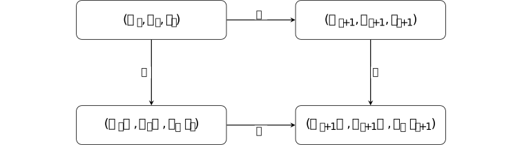
Commutation is stronger than equality of the scalar losses before the step. It states equality of the represented product trajectory after aligning the parameter bases.
Remark 5.4.1.10. Product symmetry is larger than the isometric gauge [ftip-00B5]AGENTDRAFTED
Remark 5.4.1.10. Product symmetry is larger than the isometric gauge [ftip-00B5]AGENTDRAFTED
The full \(\mathrm {GL}(k)\) action in Definition 5.4.1.2 preserves \(W\), but ordinary Euclidean gradients are covariant under the orthogonal specialization used in Lemma 5.4.1.6. A theorem for \((UQ,VQ)\) must therefore not be silently promoted to every product-preserving reparameterization.
The source calls the orthogonal subgroup the gauge in its optimizer classification while also noting the larger function-preserving group. These are compatible statements only when their different geometric scopes remain explicit.
5.4.2. Equivariant and basis-sensitive update rules [ftip-00B6]AGENTDRAFTED
5.4.2. Equivariant and basis-sensitive update rules [ftip-00B6]AGENTDRAFTED
Gradient covariance supplies a test for update rules. Linear and full-matrix operations can commute with a latent rotation, whereas a fixed nonlinear map applied separately to coordinates selects a preferred basis.
Definition 5.4.2.1. Memoryless right-equivariant update [ftip-00B7]AGENTDRAFTED
Definition 5.4.2.1. Memoryless right-equivariant update [ftip-00B7]AGENTDRAFTED
A memoryless factor-update map is a function \(\Phi :\mathbb R^{n\times k}\to \mathbb R^{n\times k}\) applied to a current gradient \(G\) without a persistent optimizer state. It is right-equivariant when
\[ \Phi (GQ)=\Phi (G)Q \qquad (G\in \mathbb R^{n\times k},\ Q\in \mathrm O(k)). \]This local definition is the input of Theorem 4.5 in The loss does not see the basis, but Adam does[singh2026lossbasis]. It does not classify stateful optimizers such as Adam.
Proposition 5.4.2.2. Gradient descent and momentum preserve the orthogonal gauge [ftip-00B8]AGENTDRAFTED
Proposition 5.4.2.2. Gradient descent and momentum preserve the orthogonal gauge [ftip-00B8]AGENTDRAFTED
Gradient descent and Polyak or Nesterov momentum are gauge-equivariant when their factor gradients, momentum buffers, schedules, and look-ahead points are transformed consistently.
Proof.
Proof.
By Lemma 5.4.1.6, \(G_t\) becomes \(G_tQ\). Gradient descent therefore sends \(U_tQ\) to \((U_t-\eta _tG_t)Q\). A momentum buffer initialized at zero and formed by linear combinations of covariant gradients transforms as \(M_tQ\); a Nesterov look-ahead point is likewise the reference look-ahead right-multiplied by \(Q\). Induction proves the claim.
Proposition 4.2(1) and its proof are in Appendix B.3 of The loss does not see the basis, but Adam does[singh2026lossbasis].
Proposition 5.4.2.3. A shared scalar second moment preserves the orthogonal gauge [ftip-00B9]AGENTDRAFTED
Proposition 5.4.2.3. A shared scalar second moment preserves the orthogonal gauge [ftip-00B9]AGENTDRAFTED
Replace Adam's entrywise second-moment denominator by one scalar whose updates depend only on gauge-invariant quantities such as the pooled mean of the squared entries of both factor gradients. With a covariant first-moment buffer, the resulting stateful update is gauge-equivariant.
Proof.
Proof.
The first moment is a linear exponential average and transforms by right multiplication by \(Q\). The pooled squared-entry mean is the joint squared Frobenius norm divided by the entry count, hence is unchanged by \(G\mapsto GQ\). Its bias correction and positive scalar denominator are unchanged, so the complete update transforms covariantly.
Proposition 4.2(2) and its proof are in Appendix B.3 of The loss does not see the basis, but Adam does[singh2026lossbasis]. The result concerns this declared shared-scalar variant, not stock Adam.
Proposition 5.4.2.4. Full-matrix Muon and Shampoo preserve the orthogonal gauge [ftip-00BA]AGENTDRAFTED
Proposition 5.4.2.4. Full-matrix Muon and Shampoo preserve the orthogonal gauge [ftip-00BA]AGENTDRAFTED
Fix one factor, write \(n\in \{d_1,d_2\}\) for its row dimension, and let \(G_t,M_t\in \mathbb R^{n\times k}\) be its gradient and Muon momentum buffer. For \(0\leq \beta <1\), \(M_{-1}=0\), and the source's linear momentum update \(M_t=\beta M_{t-1}+G_t\), Muon's direction is \(\Delta _t=\operatorname {msign}(M_t)\). Under real arithmetic this stateful update and the source's damped Shampoo update are right-equivariant. The Muon claim includes the stated finite Newton--Schulz approximations; the Shampoo claim uses its complete left and right accumulators.
Proof.
Proof.
By Lemma 5.4.1.6, the primed gradient is \(G'_t=G_tQ\). Starting from \(M'_{-1}=M_{-1}Q=0\), induction through the linear momentum update gives \(M'_t=M_tQ\). If \(M_t=A\Sigma B^{\mathsf T}\) is a compact singular-value decomposition, then \(M_tQ=A\Sigma (Q^{\mathsf T}B)^{\mathsf T}\), so \(\operatorname {msign}(M_tQ)=\operatorname {msign}(M_t)Q\). For \(\epsilon _{\rm NS}>0\), the Newton--Schulz initialization \(X_0=M_t/(\lVert M_t\rVert _F+\epsilon _{\rm NS})\) is covariant because its Frobenius normalization is invariant; each polynomial iterate formed from \(X_j\) and \(X_jX_j^{\mathsf T}\) preserves the same covariance. For Shampoo, the left accumulator is invariant while the right accumulator transforms by \(R_t\mapsto Q^{\mathsf T} R_t Q\). Orthogonal functional calculus conjugates the right matrix function, so the transformed update is the original update right-multiplied by \(Q\).
Proposition 4.2(3)--(4) and its proof are in Appendix B.3 of The loss does not see the basis, but Adam does[singh2026lossbasis]. Variable splitting, coordinatewise clipping, mixed update rules, finite precision, and different damping conventions lie outside this statement. The Muon part is stateful; it does not replace the momentum buffer by the current gradient or invoke the memoryless classification of Definition 5.4.2.1.
Proposition 5.4.2.5. Coordinatewise equivariance forces linearity [ftip-00BB]AGENTDRAFTED
Proposition 5.4.2.5. Coordinatewise equivariance forces linearity [ftip-00BB]AGENTDRAFTED
Let \(k\geq 2\) and let a memoryless update have the fixed entrywise form \(\Phi (G)_{ij}=\phi (G_{ij})\). If \(\Phi (GQ)=\Phi (G)Q\) for every \(G\) and \(Q\in \mathrm O(k)\), then \(\phi (x)=cx\) for some \(c\in \mathbb R\).
Proof.
Proof.
It suffices to use one row and rotations in the first two coordinates. Equivariance at zero gives \(\phi (0)=0\). Rotating \((x,0)\) through an angle whose cosine is \(a\in [-1,1]\) gives \(\phi (ax)=a\phi (x)\). For nonzero \(x,y\), compare each with a third number of at least their absolute magnitudes; the ratio \(\phi (x)/x\) is constant.
Proposition 4.3 and its proof are in Appendix B.4 of The loss does not see the basis, but Adam does[singh2026lossbasis]. No continuity assumption is needed.
Corollary 5.4.2.6. Fixed nonlinear coordinatewise updates break the gauge [ftip-00BC]AGENTDRAFTED
Corollary 5.4.2.6. Fixed nonlinear coordinatewise updates break the gauge [ftip-00BC]AGENTDRAFTED
A nonlinear fixed entrywise update applied at a zero optimizer state is not gauge-equivariant when \(k\geq 2\). In particular, the source applies Proposition 5.4.2.5 to the first-step maps of Adam, RMSProp, signSGD, and Lion; it checks Adafactor separately because its factored statistics are not an entrywise map.
This is a first-step obstruction. It suffices to disprove equivariance of the full run, but it does not classify every later state or say that such an optimizer cannot reach a particular solution.
Definition 5.4.2.7. First-step Adam map and gauge defect [ftip-00BD]AGENTDRAFTED
Definition 5.4.2.7. First-step Adam map and gauge defect [ftip-00BD]AGENTDRAFTED
Fix \(\epsilon >0\). For zero-state, bias-corrected Adam define the entrywise first-step direction
\[ D_\epsilon (G)=G\mathbin {\oslash }(|G|+\epsilon ) \]and, for \(Q\in \mathrm O(k)\), define its gauge-aligned defect by
\[ E_Q(G)=D_\epsilon (GQ)Q^{\mathsf T}-D_\epsilon (G). \]Here \(|G|\), addition, and division are entrywise. Bias correction makes the first direction independent of Adam's two decay coefficients under the declared convention [singh2026lossbasis, Proposition 4.4].
Proposition 5.4.2.8. Exact represented-matrix defect after one Adam step [ftip-00BE]AGENTDRAFTED
Proposition 5.4.2.8. Exact represented-matrix defect after one Adam step [ftip-00BE]AGENTDRAFTED
Let \(G_U=\nabla _UL(U_0,V_0)\), \(G_V=\nabla _VL(U_0,V_0)\), \(D_U=D_\epsilon (G_U)\), and \(D_V=D_\epsilon (G_V)\). Let \(W_1\) be the product after one Adam step from \((U_0,V_0)\) and \(\widetilde W_1\) the product after one step from \((U_0Q,V_0Q)\). Then
\[ \begin {aligned} \widetilde W_1-W_1={}&-\eta \bigl (E_Q(G_U)V_0^{\mathsf T} +U_0E_Q(G_V)^{\mathsf T}\bigr )\\ &+\eta ^2\bigl (E_Q(G_U)D_V^{\mathsf T} +D_UE_Q(G_V)^{\mathsf T} +E_Q(G_U)E_Q(G_V)^{\mathsf T}\bigr ). \end {aligned} \]
Proof.
Proof.
Gauge-align the rotated factors back by \(Q^{\mathsf T}\). They are \(U_0-\eta (D_U+E_Q(G_U))\) and \(V_0-\eta (D_V+E_Q(G_V))\). Multiply, subtract \((U_0-\eta D_U)(V_0-\eta D_V)^{\mathsf T}\), and collect powers of \(\eta \).
Proposition 4.4 and its proof are in Appendix B.5 of The loss does not see the basis, but Adam does[singh2026lossbasis].
Example 5.4.2.9. A two-coordinate Adam defect witness [ftip-00BF]AGENTDRAFTED
Example 5.4.2.9. A two-coordinate Adam defect witness [ftip-00BF]AGENTDRAFTED
Take \(d_1=d_2=1\), \(k=2\), \(f(w)=w^2/2\), \(U_0=V_0=(1,0)\), and
\[ Q=2^{-1/2}\begin {pmatrix}1&1\\-1&1\end {pmatrix}. \]The original and rotated products after one zero-state Adam step are
\[ W_1=\left (1-\frac {\eta }{1+\epsilon }\right )^2, \qquad \widetilde W_1=\left (1-\frac {\eta }{2^{-1/2}+\epsilon }\right )^2. \]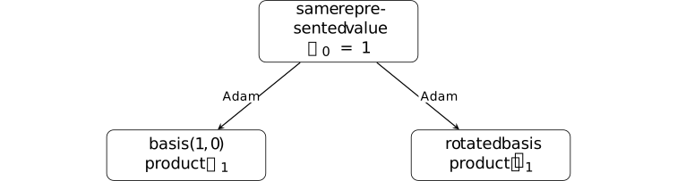
They differ when \(0<\eta <2^{-1/2}+\epsilon \). This is the explicit witness in Proposition 4.4 of The loss does not see the basis, but Adam does[singh2026lossbasis]; it is a statement about one factored quadratic, not about language-model performance.
Example 5.4.2.10. A rotated sign update fails to commute [ftip-00BG]AGENTDRAFTED
Example 5.4.2.10. A rotated sign update fails to commute [ftip-00BG]AGENTDRAFTED
For \(G=(1,1)\) and the 45-degree rotation matrix \(Q\) of Example 5.4.2.9, one has \(GQ=(0,\sqrt 2)\). With \(\operatorname {sign}(0)=0\),
\[ \operatorname {sign}(GQ)=(0,1), \qquad \operatorname {sign}(G)Q=(0,\sqrt 2). \]Thus even this two-coordinate update violates the commuting equation in Definition 5.4.2.1. The calculation is the explicit Appendix B.4 witness of The loss does not see the basis, but Adam does[singh2026lossbasis].
Theorem 5.4.2.11. Full-rank memoryless equivariant rules are Gram-determined [ftip-00BH]AGENTDRAFTED
Theorem 5.4.2.11. Full-rank memoryless equivariant rules are Gram-determined [ftip-00BH]AGENTDRAFTED
Let \(k\leq n\), and let \(\Phi \) be defined on full-column-rank matrices \(G\in \mathbb R^{n\times k}\). Then \(\Phi (GQ)=\Phi (G)Q\) for every \(Q\in \mathrm O(k)\) if and only if there is a matrix-valued function \(H\) of \(GG^{\mathsf T}\) such that
\[ \Phi (G)=H(GG^{\mathsf T})G. \]
Proof.
Proof.
The displayed form is immediately equivariant. Let \(G^+\) denote the Moore--Penrose pseudoinverse. Conversely, set \(X(G)=\Phi (G)G^+\). Then \(X(G)G=\Phi (G)\) and \(X(GQ)=X(G)\). Two full-column-rank matrices with the same left Gram matrix have the same range and differ by a right orthogonal factor. Hence \(X(G)\) depends only on \(GG^{\mathsf T}\); take \(H=X\).
See Theorem 4.5 and its proof in Appendix B.6 of The loss does not see the basis, but Adam does[singh2026lossbasis]. It classifies the full-rank stratum only.
Corollary 5.4.2.12. The square invertible preconditioner representation [ftip-00BI]AGENTDRAFTED
Corollary 5.4.2.12. The square invertible preconditioner representation [ftip-00BI]AGENTDRAFTED
In the specialization \(k=n\) with \(G\) invertible, let \(P^{1/2}\) denote the unique positive-definite square root of \(P\). The function in Theorem 5.4.2.11 has the unique canonical representative
\[ H(P)=\Phi (P^{1/2})P^{-1/2}, \qquad P=GG^{\mathsf T}>0. \]
Proof.
Proof.
The polar decomposition writes \(G=P^{1/2}Q\). Equivariance gives \(\Phi (G)=\Phi (P^{1/2})Q=H(P)G\). Evaluating at \(G=P^{1/2}\) proves uniqueness in this square invertible case.
For rectangular \(G\), the action of \(H(P)\) away from the range needed to multiply \(G\) is not determined by \(\Phi \). The proof above establishes uniqueness in the square invertible specialization.
Remark 5.4.2.13. What the structure theorem leaves unresolved at rank deficiency [ftip-00BJ]AGENTDRAFTED
Remark 5.4.2.13. What the structure theorem leaves unresolved at rank deficiency [ftip-00BJ]AGENTDRAFTED
In the ambient matrix space, full-column-rank matrices form an open dense subset whose complement has Lebesgue measure zero. A probability-one claim requires the random gradient law to be absolutely continuous and not confined to a lower-rank set; random initialization alone does not supply that premise.
Theorem 5.4.2.11 therefore makes no classification claim on a general rank-deficient stratum. Equivariance still constrains values within each orthogonal orbit, and it forces \(\Phi (0)=0\), but it does not determine the rule there by continuity unless continuity is separately assumed. The source's generic-rank discussion therefore does not establish a classification at rank deficiency.
5.4.3. Common-scalar flows, clock changes, and momentum [ftip-00BK]AGENTDRAFTED
5.4.3. Common-scalar flows, clock changes, and momentum [ftip-00BK]AGENTDRAFTED
One narrow class of continuous-time preconditioners follows the gradient-flow path at a different speed. The clock change transfers path properties, but not rates, and it does not encompass a stateful momentum method.
Definition 5.4.3.1. Common-scalar preconditioned flow [ftip-00BL]AGENTDRAFTED
Definition 5.4.3.1. Common-scalar preconditioned flow [ftip-00BL]AGENTDRAFTED
Let \(\theta =(U,V)\) and let \(a(t)>0\) be measurable with \(1/a\) locally integrable. A common-scalar preconditioned flow is a locally absolutely continuous trajectory satisfying
\[ \dot \theta (t)=-\frac {\nabla L(\theta (t))}{a(t)} \]for almost every \(t\). The same scalar multiplies every coordinate of both factor gradients. For gauge-uniform conclusions, the source additionally requires \(a(t)\) to be determined by gauge-invariant statistics of the trajectory up to time \(t\).
Definition 5.4.3.2. Effective optimizer clock [ftip-00BM]AGENTDRAFTED
Definition 5.4.3.2. Effective optimizer clock [ftip-00BM]AGENTDRAFTED
For the flow of Definition 5.4.3.1, define the effective optimizer clock
\[ \tau (t)=\int _0^t\frac {du}{a(u)}, \qquad \tau _{\max }=\int _0^\infty \frac {du}{a(u)}, \qquad 0<\tau _{\max }\leq \infty . \]The clock is strictly increasing on its domain. If \(\tau _{\max }=\infty \), it reaches every gradient-flow time; otherwise it traverses only the prefix with effective time below \(\tau _{\max }\).
Theorem 5.4.3.3. Common-scalar flow is a time-reparameterized gradient flow [ftip-00BN]AGENTDRAFTED
Theorem 5.4.3.3. Common-scalar flow is a time-reparameterized gradient flow [ftip-00BN]AGENTDRAFTED
Let \(\theta (t)\) satisfy Definition 5.4.3.1, let \(t(\tau )\) be the inverse of the clock in Definition 5.4.3.2, and put \(\widetilde \theta (\tau )=\theta (t(\tau ))\). Then, for almost every \(\tau \),
\[ \widetilde \theta '(\tau )=-\nabla L(\widetilde \theta (\tau )). \]
Proof.
Proof.
The chain rule for absolutely continuous changes of variable gives \(dt/d\tau =a(t)\) almost everywhere. Multiplying \(\dot \theta =-\nabla L/a(t)\) by \(dt/d\tau \) yields the displayed gradient flow.
See Theorem 4.6 and its proof in Appendix B.9 of The loss does not see the basis, but Adam does[singh2026lossbasis]. Gauge invariance of \(a\) is not needed for this single-trajectory clock identity; it makes the clock common across a gauge orbit.
Corollary 5.4.3.4. Transfer of path and limit properties [ftip-00BO]AGENTDRAFTED
Corollary 5.4.3.4. Transfer of path and limit properties [ftip-00BO]AGENTDRAFTED
Every property depending only on the portion of the gradient-flow path traversed before \(\tau _{\max }\) transfers to the common-scalar flow. If \(\tau _{\max }=\infty \) and gradient flow converges, both flows have the same limit point. A sufficient condition for clock divergence is an eventual finite upper bound on \(a(t)\).
For shallow factorization, the source cites Implicit regularization in matrix factorization[gunasekar2017implicit]. For deep factorization, it cites Implicit regularization in deep matrix factorization[arora2019implicit]. For greedy low-rank dynamics, it cites Towards resolving the implicit bias of gradient descent for matrix factorization: Greedy low-rank learning[li2021greedy].
Those conclusions transfer only when both this clock theorem and every hypothesis of the original result hold. This corollary supplies no missing matrix-sensing assumption.
Remark 5.4.3.5. Rates and hitting times do not survive time reparameterization [ftip-00BP]AGENTDRAFTED
Remark 5.4.3.5. Rates and hitting times do not survive time reparameterization [ftip-00BP]AGENTDRAFTED
Two flows can traverse the same curve with arbitrarily different physical clocks. A convergence rate, finite-step budget, or hitting time stated in \(t\) therefore does not transfer through Theorem 5.4.3.3 without quantitative bounds on \(a\) and its integral. If \(\tau _{\max }<\infty \), even the tail and limit of the gradient-flow path are not reached.
Remark 5.4.3.6. Scalar-Adam is outside the common-scalar flow theorem [ftip-00BQ]AGENTDRAFTED
Remark 5.4.3.6. Scalar-Adam is outside the common-scalar flow theorem [ftip-00BQ]AGENTDRAFTED
The shared-scalar Adam variant in Proposition 5.4.2.3 retains a first-moment exponential moving average. It is stateful and is not the memoryless flow in Definition 5.4.3.1. Remark 4.7 of The loss does not see the basis, but Adam does[singh2026lossbasis] treats its agreement with gradient flow as empirical rather than as a consequence of Theorem 4.6.
The theorem likewise does not apply to discrete Adam, PPO, RLVR update loops, clipping, weight decay, and mixed optimizers. Gauge equivariance and time reparameterization are separate properties.
Example 5.4.3.7. Equivariance neither guarantees nor precludes recovery [ftip-00BR]AGENTDRAFTED
Example 5.4.3.7. Equivariance neither guarantees nor precludes recovery [ftip-00BR]AGENTDRAFTED
The source records controls on both sides of the proposed implication. Its ScaledGD-inspired control is equivariant but equalizes the spectral schedule and does not recover the planted low-rank target at the declared budget. A long-anneal sign update is non-equivariant but eventually reaches a low-recovery-error regime.
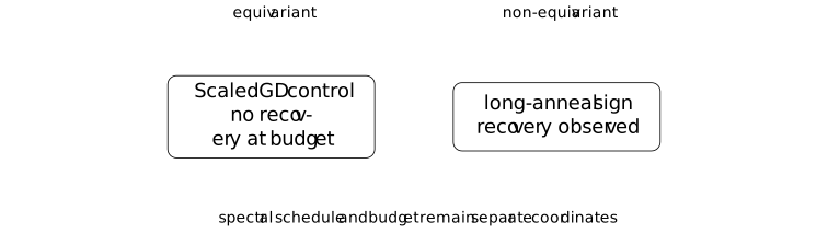
The controls are reported in Remark 4.7 and Appendix D.10 of The loss does not see the basis, but Adam does[singh2026lossbasis]. The source reports no tuned reproducibility baseline for the ScaledGD control. The diagram is not a convergence theorem.
5.4.4. Optimizer geometry in training interventions [ftip-00BS]AGENTDRAFTED
5.4.4. Optimizer geometry in training interventions [ftip-00BS]AGENTDRAFTED
Equivalent parameterizations need not follow equivalent training trajectories. Their evolution also depends on the update geometry; the scalar loss and represented starting object do not always suffice.
Definition 5.4.4.1. Objective-equivalent parameterizations [ftip-00BT]AGENTDRAFTED
Definition 5.4.4.1. Objective-equivalent parameterizations [ftip-00BT]AGENTDRAFTED
Two factor pairs \((U,V)\) and \((\widetilde U,\widetilde V)\) are objective-equivalent for \(L=f\circ W\) when
\[ W(U,V)=W(\widetilde U,\widetilde V). \]They then have the same scalar loss for every objective depending only on that represented matrix. Orthogonal gauge-related pairs are objective-equivalent by Lemma 5.4.1.3; objective equivalence need not imply membership in the same orthogonal orbit.
Definition 5.4.4.2. Parameterization-stable training intervention [ftip-00BU]AGENTDRAFTED
Definition 5.4.4.2. Parameterization-stable training intervention [ftip-00BU]AGENTDRAFTED
Fix a factorized objective, an update algorithm, hyperparameter schedule, randomness coupling, stopping rule, and initial optimizer state. The resulting training intervention is parameterization-stable on an orthogonal orbit when every two gauge-related initial states have identical represented trajectories:
\[ \widetilde U_t\widetilde V_t^{\mathsf T}=U_tV_t^{\mathsf T} \qquad \hbox {at every compared step }t. \]This is a local stability property of a fully declared intervention. It does not say that arbitrary objective-equivalent pairs outside the orbit must agree.
Proposition 5.4.4.3. Gauge equivariance gives parameterization stability [ftip-00BV]AGENTDRAFTED
Proposition 5.4.4.3. Gauge equivariance gives parameterization stability [ftip-00BV]AGENTDRAFTED
Every gauge-equivariant optimizer is parameterization-stable on each orthogonal orbit, provided the remaining protocol coordinates are coupled as in Definition 5.4.4.2.
Proof.
Proof.
Definition 5.4.1.8 gives \((\widetilde U_t,\widetilde V_t)=(U_tQ,V_tQ)\). Hence
\[ \widetilde U_t\widetilde V_t^{\mathsf T} =U_tQQ^{\mathsf T}V_t^{\mathsf T}=U_tV_t^{\mathsf T}. \]This is a sufficient condition on a declared orbit, not a claim that equivariance is necessary for every possible equality of represented trajectories.
Proposition 5.4.4.4. A first-step defect falsifies a loss-only protocol specification [ftip-00BW]AGENTDRAFTED
Proposition 5.4.4.4. A first-step defect falsifies a loss-only protocol specification [ftip-00BW]AGENTDRAFTED
Suppose two orthogonally gauge-related initializations have equal represented object and scalar objective, but a declared update produces different represented objects after one step. Then the training intervention is not determined by the represented initialization and scalar objective alone.
Proof.
Proof.
If those two objects determined the intervention, equal inputs would give the same represented next state. The witnessed inequality contradicts that factorization.
Proposition Proposition 5.4.2.8 and Example 5.4.2.9 instantiate its premise for one factored quadratic and zero-state Adam. It proves underspecification, not a capability difference.
Example 5.4.4.5. The orthogonal gauge of an attention head [ftip-00BX]AGENTDRAFTED
Example 5.4.4.5. The orthogonal gauge of an attention head [ftip-00BX]AGENTDRAFTED
For the row-vector attention weights of Definition 5.1.5, let \(W^Q,W^K\in \mathbb R^{d\times d_h}\) and \(Q_h=XW^Q\), \(K_h=XW^K\). Attention logits depend on these weights through
\[ Q_hK_h^{\mathsf T}=XW^Q(W^K)^{\mathsf T}X^{\mathsf T}. \]For \(A\in \mathrm O(d_h)\), the right action \((W^Q,W^K)\mapsto (W^QA,W^KA)\) preserves the middle product.

Section 6 of The loss does not see the basis, but Adam does[singh2026lossbasis] uses column-vector weights and the invariant \(W_Q^{\mathsf T}W_K\). Transposition gives the row-vector invariant \(W^Q(W^K)^{\mathsf T}\), with the action on the right as displayed.
Remark 5.4.4.6. What the attention-twin experiment observes [ftip-00BY]AGENTDRAFTED
Remark 5.4.4.6. What the attention-twin experiment observes [ftip-00BY]AGENTDRAFTED
Section 6 and Table 3 of The loss does not see the basis, but Adam does[singh2026lossbasis] compare two function-equivalent initializations of a two-layer, four-head transformer on modular addition. The reported relative logit distance after one Adam step is \(3.6\times 10^{-3}\), versus \(2.9\times 10^{-7}\) for a same-basis noise twin; the final per-head invariant distance is reported as 56 percent.
The exact first-step defect has an algebraic explanation, but later drift, scale robustness, and downstream behavior are empirical. The tested small transformers, precision, optimizer allocation, seeds, and task do not establish a frontier-wide law.
Example 5.4.4.7. One loss quotient and two optimizer trajectories [ftip-00BZ]AGENTDRAFTED
Example 5.4.4.7. One loss quotient and two optimizer trajectories [ftip-00BZ]AGENTDRAFTED
A loss-only description collapses a gauge orbit to one represented starting point. A basis-sensitive optimizer can split that quotient back into different represented trajectories.
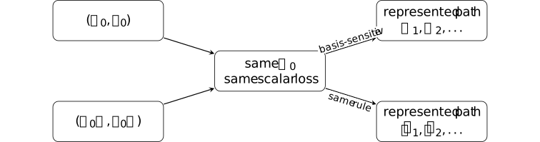
The right-hand split is possible only because the centre box omits the factor basis and optimizer geometry. An FTIP admissible protocol in Definition 4.1.7 must retain those intervention coordinates when they affect the executable result.
Remark 5.4.4.8. Product symmetry and the scope of optimizer conclusions [ftip-00C0]AGENTDRAFTED
Remark 5.4.4.8. Product symmetry and the scope of optimizer conclusions [ftip-00C0]AGENTDRAFTED
The relevant optimizer results appear in version 1 of [⧉], submitted 5 August 2026: Sections 3--4 and 6, Appendices B.1--B.6 and B.9, with limitations in Section 11.
The full product symmetry acts on the factors by
\[ (U,V)\longmapsto (UA,VA^{-\mathsf T}). \]It does not use \((UA,VA)\). For row-vector attention weights, the corresponding action uses right multiplication, as in Example 5.4.4.5.
The general rectangular preconditioner representation need not have the square-case uniqueness. A probability-one full-rank claim additionally needs a law for the gradient; a generic full-rank observation does not specify one.
The coordinatewise theorem is a zero-state, memoryless obstruction. The clock theorem is continuous-time and excludes scalar-Adam's momentum. Experimental optimizer and attention results remain observations reported by the source. Equivariance is not identified with low-rank recovery.
Remark 5.4.4.9. Continuous-flow conclusions and discrete optimization [ftip-00C1]AGENTDRAFTED
Remark 5.4.4.9. Continuous-flow conclusions and discrete optimization [ftip-00C1]AGENTDRAFTED
The factored-model results prove that update geometry can be a genuine intervention coordinate even when objective and represented initialization are fixed. They do not prove transformer or RLVR convergence, practical optimizer superiority, a scaling law, or any change in reliable capability. Different represented trajectories are not by themselves an acquisition witness of Definition 4.3.4.
The memoryless theorem does not describe Adam's full state, and the continuous-flow result does not supply discrete rates or finite-step bounds. The source also notes that fixed-rank LoRA changes the learned-rank mechanism; no LoRA transfer is made here.
A dynamic-compute comparison also depends on active research state, persistent harness state, retained history, evaluation configuration, and descendant and retry costs. One realized chain and an archive-best envelope are different outcomes, even at the same declared budget.
6. Conceptual discovery across model generations [ftip-00MH]AGENTDRAFTED
6. Conceptual discovery across model generations [ftip-00MH]AGENTDRAFTED
The preceding chapters specify the model and learning mechanisms, retained agent state, evaluation and costs, with architecture-dependent refinements when needed. This chapter combines them in a question about capability growth across successive learned artifacts.
A mathematical breakthrough may require a new representation, a useful invariant, or a connection to another domain. The question is whether a specified model lineage can discover and acquire that structure within its resources, including by improving its own search and training procedures. An external contribution might make the same capability affordable.
This is a proposed separation between complete processes. A plateau in one training recipe does not establish it. Nor does the size of unexplored mathematics imply that current architectures can only recombine a fixed stock of ideas. Useful structure may be generated implicitly by updates, through analogy, or by programs constructed during the campaign.
The acquisition question in Definition 1.1.5 therefore extends across successive learned artifacts. The finite discovery estimates of § 4.4.1 apply only when their probability premises cover that evolving process. The finite controller certificate in § 3.1.5.2 illustrates an upper-bound method for a fully specified action class.
6.1. The complete lineage and its resources [ftip-00MI]AGENTDRAFTED
6.1. The complete lineage and its resources [ftip-00MI]AGENTDRAFTED
The comparison starts from disclosed artifacts and executable operations. A lineage includes the models it trains, the controllers it writes, and the evidence it retains. Its limits cannot be inferred from the support of one initial decoder while allowing the rest of the system to change.
Definition 6.1.1. A resource-bounded model lineage [ftip-00MJ]AGENTDRAFTED
Definition 6.1.1. A resource-bounded model lineage [ftip-00MJ]AGENTDRAFTED
Fix a specification
\[ \Xi =(I_0,\mathcal C_0,\Gamma ,\mathcal E_0,V, \mathcal D,\mathcal F,\mathbf B,\mathbf b_{\mathrm {eval}}). \]Here \(I_0\) contains the initial models, corpora, libraries, prompts, optimizers, evaluators, software and cached results. The nonempty class \(\mathcal C_0\) specifies controller programs and constants available from \(I_0\); it does not grant an arbitrary program chosen after a discovery. An initial generator of additional controllers is allowed, with its generation and selection work charged as explained in Convention 6.5.1. The semantics \(\Gamma \) specifies executable operations and costs; \(\mathcal E_0\) specifies baseline observations and tool-response laws. The checker \(V\), task law and reveal schedule \(\mathcal D\), allowed final artifacts \(\mathcal F\), campaign cap \(\mathbf B\) and deployment cap \(\mathbf b_{\mathrm {eval}}\) are fixed before evaluation. Include the no-update procedure as a baseline.
A campaign is a causal execution starting from this endowment. Its state contains available checkpoints, contexts, generated code, retained traces, libraries, optimizer state and resource usage. A controller may use only its charged accessible state: discarded history must be reconstructed at cost. Environment state may remain hidden. All random seeds follow their declared laws; a fortunate completed trajectory is not an available program.
Whenever admitted by \(\Gamma \), operations include model inference, proof and program search, tool calls, parallel workers, memory management, candidate comparison, reward and credit assignment, synthetic tasks, parameter training, architecture changes, and controller replacement. Generated controllers execute under the same semantics and caps. Selection, evaluation and the controller's own computation are charged. These operations may recur in any order; learning need not first produce a complete successful trace or an explicitly verbalized idea.
The lineage is closed relative to \((I_0,\mathcal E_0)\) when its only campaign inputs are scheduled tasks, its randomness and admitted environment responses. This allows computation to reveal useful structure. A simulator using independent randomness is different from a tool observing new hidden world state; the latter access belongs in \(\mathcal E_0\).
Controller selection is independent of unrevealed instance seeds, conditional on declared public family information. This alone does not exclude family-wide answer tables: all such constants and preprocessing belong in \(I_0\). An asymptotic claim specifies uniform generation across instance sizes or explicitly accounts for nonuniform advice and preparation.
Definition 6.1.2. Hard resource accounting across generations [ftip-00MK]AGENTDRAFTED
Definition 6.1.2. Hard resource accounting across generations [ftip-00MK]AGENTDRAFTED
For a realized campaign \(\zeta \), let \(\mathbf R(\zeta )\) record inference work, training work, tool and checker work, total accelerator time, peak live memory and storage, peak allocated hardware, wall time and money under the declared operational model. Admission requires
\[\mathbf R(\zeta )\preceq \mathbf B\quad \text {almost surely}.\]Stop before an unaffordable operation; a missing result scores zero. Charge every failed path, discarded trace, evaluator call, consultation, checkpoint comparison and update. Bound the number of transitions by charged elementary work or an explicit finite horizon: infinitely many free operations are not admitted.
For additive work coordinates, a portfolio costs shared development plus the sum of task-specific work. Shared training is charged once even when it benefits many tasks. Peak resources and elapsed time come from the actual joint schedule, including communication and sequential dependencies. Parallel work is summed across workers. An expected-cost bound does not replace this hard cap.
A scalar budget \(B\) is used only after choosing one resource or a declared conversion with the remaining constraints fixed. Human time, accelerator work and elapsed time have no implicit exchange rate. Model pretraining and contributor expertise may be disclosed sunk endowments in a marginal comparison. A lifetime-cost claim must also account for producing both; unknown historical costs remain unknown.
6.2. Discovery and acquired capability [ftip-00ML]AGENTDRAFTED
6.2. Discovery and acquired capability [ftip-00ML]AGENTDRAFTED
A contribution can help solve a current problem without becoming a reusable ability. Discovery and acquisition are therefore separate outcomes, both evaluated against a fixed mathematical truth contract.
Definition. Signed discovery and fresh-task acquisition [ftip-00MM]AGENTDRAFTED
Definition. Signed discovery and fresh-task acquisition [ftip-00MM]AGENTDRAFTED
Fix the statement translation, allowed axioms, formal library and certificate checker \(V\). An answer is a sign \(\sigma \in \{+,-\}\) and a certificate \(p\). Put \(s_V(x,(\sigma ,p))=1\) when \(V\) accepts \(p\) as a proof of \(x\) for sign \(+\), or of \(\neg x\) for sign \(-\); otherwise put \(s_V=0\). The failure output \(\bot \) scores zero. A proof of excluded middle without either signed certificate does not solve the task. A task family may assume one signed certificate exists; independence from the allowed axioms is otherwise a separate source of failure.
For a current portfolio \(x_1,\ldots ,x_n\) with fixed nonnegative weights \(w_i\) summing to one, a campaign \(P\) has discovery score
\[Q_{\mathrm {disc}}(P)=\mathbb E\sum _{i=1}^n w_i s_V(x_i,P_i).\]For one fixed conjecture use a singleton portfolio; its truth need not be randomized. The expectation includes the declared task and execution randomness, with no assumption of independent attempts.
After development, freeze an artifact \(A\in \mathcal F\cup \{\bot \}\) before revealing fresh problems \(x'_1,\ldots ,x'_m\), where \(m\geq 1\). Their identities and solutions are unavailable during development; they are conditionally independent of development draws given the declared task-family variable. With a fixed deployment procedure \(\mathrm {Deploy}\), define
\[ Q_{\mathrm {acq}}(P)=\mathbb E\frac 1m\sum _{j=1}^m s_V(x'_j,\mathrm {Deploy}(A,x'_j;\mathbf b_{\mathrm {eval}})). \]Remove contributor access and feedback into training or checkpoint selection. Any permitted adaptation within one test problem is charged and discarded before the next. Evaluation work counts in the campaign; the per-problem cap is common to both arms. Deployment of \(\bot \) fails.
For model acquisition, \(\mathcal F\) contains learned parameters or adapters with a common fixed harness. For system acquisition it may instead include a bounded acquired library or controller. State which is measured. The pair \((Q_{\mathrm {disc}},Q_{\mathrm {acq}})\) does not allow success on one coordinate to conceal failure on the other. Imported mathematical results and new proof notation require sound translation under \(V\), including the cost of expanding and checking certificates.
6.3. Affordable complementary contributions [ftip-00MT]AGENTDRAFTED
6.3. Affordable complementary contributions [ftip-00MT]AGENTDRAFTED
The recipient is the learning system that receives and processes a contribution. Its interaction protocol specifies the permitted tools, retained state and update procedures. The contributor is the source of that contribution.
A contributor can make a representation, analogy, criticism, discriminating question or research direction affordably available to a recipient. The relevant properties are the interaction it can produce and what the recipient can make of it. Architecture, culture, expertise and developmental history can explain these properties without becoming mandatory coordinates of the abstract definition.
Availability, structural quality and realized benefit require different arguments. A familiar connection can be novel to a learner's affordable repertoire, while a surprising sentence may be useless. The existence of infinitely many possible patterns supplies neither a probability of useful help nor an unaided computational lower bound.
Definition 6.3.1. A causal contribution process [ftip-00MU]AGENTDRAFTED
Definition 6.3.1. A causal contribution process [ftip-00MU]AGENTDRAFTED
Fix the recipient specification, task family, reveal schedule, interaction permissions and resource accounting. Abstract a contributor \(v\) by a causal interaction law, written as budget-indexed kernels
\[K_v^b(\mathrm dh\mid H).\]Here \(H\) is the history available to the contributor, \(b\) is its remaining contribution budget, and \(h\) includes the next message or failure/stop output with its joint resource record. The kernels arise from one consistent causal process under stopping: different budgets cannot be assigned unrelated ideal answers. No access to unrevealed test instances or their answers is permitted.
Two internal realizations are equivalent for this abstraction when they induce the same joint laws of transcripts, costs and stopping for every admitted recipient protocol and budget. Mathematically equivalent message contents need not be equivalent interactions: the recipient may find one encoding much easier to interpret or verify. A useful contribution may develop through several exchanges. Producing, interpreting, rejecting, correcting and learning from suggestions all consume resources.
Conditional theorems may assume properties of this interface without simulating a brain or reconstructing a civilization. An unconditional existence result additionally requires a realizable member of the assumed class, for example an executable source with disclosed initial state and costs. A controlled human protocol instead supplies empirical estimates. An arbitrary answer kernel or assumed success probability proves neither.
The target statements, truth contract, checker and reveal schedule stay fixed. Contributors may have different broad backgrounds or search biases; these endowment differences are disclosed. Relevant prior results must be justified under the target checker. A hidden target parameter or precomputed answer table is a different mechanism from conceptual insight. Equalizing all background material is an optional stronger comparison. Giving the recipient textual access to the relevant material can test whether acquiring and using the connection remains costly. Historical preparation follows the symmetric accounting convention in Definition 6.1.2.
Definition 6.3.2. Structural quality and good contributor classes [ftip-00MV]AGENTDRAFTED
Definition 6.3.2. Structural quality and good contributor classes [ftip-00MV]AGENTDRAFTED
Fix a development law and recipient interaction protocol \(\Pi \) before final evaluation. For development input \(D\) and resulting contribution transcript \(H_v\), choose an independently specified structural predicate \(S(D,H_v)\). Define
\[q_v=\Pr _{\Pi ,v}\bigl (S(D,H_v)\bigr ).\]A possible property is a sound reduction to a declared tractable class with bounded translation and certificate-expansion costs. A reusable invariant with a proved consequence or a curriculum satisfying a separate learning condition are other possibilities. A fallible analogy may require charged recipient completion before the property holds. The predicate is not simply that the final score improved; soundness, scope and checking costs require their own arguments. Quality is relative to this task, protocol and budget, not a universal ranking of minds.
For \(0<q_0\leq 1\), the restricted class
\[\mathcal G(q_0)=\{v\in \mathfrak V:q_v\geq q_0\}\]is legitimate. An existence theorem about a member of this class need not help every contributor outside it. Nonemptiness remains a separate obligation; choosing sources on final test outcomes does not establish pre-evaluation availability. Recruitment and screening costs are necessary when claiming an affordable procedure to find a good contributor, but mere existence does not require a population recruitment theorem.
To discuss a median, additionally declare a population law \(\mu \) on admissible contributors with measurable quality \(v\mapsto q_v\). Let \(q_{50}\) satisfy \(\mu (q_v\leq q_{50})\geq \frac 12\) and \(\mu (q_v\geq q_{50})\geq \frac 12\). Then define
\[\mathcal G_\mu (q_0)=\{v:q_v\geq \max (q_0,q_{50})\}.\]If \(q_0\leq q_{50}\), this class has at least half the population mass. If \(q_0>q_{50}\), even nonemptiness needs evidence. The median can be zero, so belonging to the upper half alone does not guarantee useful assistance. There is no default uniform law over all possible contributors, and an unattained quality supremum need not have a best contributor.
Proposition 6.3.3. From structural quality to acquired capability [ftip-00MW]AGENTDRAFTED
Proposition 6.3.3. From structural quality to acquired capability [ftip-00MW]AGENTDRAFTED
Fix one contributor and one recipient protocol with almost-sure total resource caps, including failed consultations. Let \(Z\in [0,1]\) be the realized fresh-task score of its frozen artifact with contributor access removed. Suppose, for the same joint process and remaining resources,
\[\Pr (S)\geq q_0>0,\qquad \mathbb E[Z\mid S]\geq \beta \geq 0.\]Then \(Q_{\mathrm {acq}}=\mathbb E Z\geq q_0\beta \).
Proof.
Proof.
Nonnegativity and conditional expectation give
\[\mathbb E Z\geq \mathbb E[Z\mathbf 1_S] =\Pr (S)\mathbb E[Z\mid S]\geq q_0\beta .\]No independence assumption is used. A uniform recipient guarantee for qualified transcripts and compatible development histories can establish the transfer premise, including interpretation, verification and acquisition costs. A guarantee for a different, easier message distribution cannot.
Together with a universal closed bound \(Q_{\mathrm {acq}}(P)\leq \tau ^-\) and an admissible member of \(\mathcal G(q_0)\), the strict inequality \(q_0\beta \geq \tau ^+>\tau ^-\) yields the assisted crossing in Conjecture 6.4. The substantive obligations are affordable source quality, recipient transfer and the bound over every admitted unaided alternative. The elementary expectation inequality alone establishes none of these.
Proposition 6.3.4. Simulation can erase an apparent contribution advantage [ftip-00MX]AGENTDRAFTED
Proposition 6.3.4. Simulation can erase an apparent contribution advantage [ftip-00MX]AGENTDRAFTED
Fix a scalar accounting model with the other constraints declared. Suppose an admitted assisted campaign \((R,v)\) at total budget \(B\) has an admitted closed simulator at budget \(g(B)\). Require that the simulator can reproduce the contributor's endowment, observations and causal interaction, together with the recipient's allowed final artifact and evaluation law. All simulation work and initialization count. Then, for \(j\in \{\mathrm {disc},\mathrm {acq}\}\),
\[\sup _{P\in \mathcal L(g(B))}Q_j(P)\geq Q_j(R,v).\]
Proof.
Proof.
Couple the initial states and each successive conditional interaction using the stipulated simulator. Induction gives the same joint law of observable transcripts, final artifact and evaluated outcomes. The closed simulator therefore has the same score, and its admission places that score below the displayed supremum.
If the simulation is uniform across instance sizes with \(g(B)\leq cB\) for a fixed constant \(c\), an actual assisted procedure reaching \(\tau \) at work \(U(n)\) implies \(B_{\mathrm {closed}}(n,\tau )\leq cU(n)\). This excludes a lower bound \(L(n)\) with \(U(n)/L(n)\to 0\). Unavailable background state, observations, hardware or large simulation overhead can invalidate the premise; different origin alone does not. The argument does not assume that a language model already has an affordable simulation of a human contributor.
Admission includes discovery of any required reconstruction program from the declared initial state. A simulator written with advance knowledge of the useful representation does not satisfy this premise merely because its later execution is cheap. If the program is generated during the campaign, its generation law, failed attempts and selection costs belong in the simulation. This conditional proposition supplies no lower bound on that discovery cost; Convention 6.5.1 distinguishes program existence from its availability to the lineage.
Example 6.3.5. A human–agent exchange about conceptual discovery [ftip-00MY]AGENTDRAFTED
Example 6.3.5. A human–agent exchange about conceptual discovery [ftip-00MY]AGENTDRAFTED
In this exchange, the human is the contributor and the agent is the recipient: the system receiving and processing the contribution. The agent's proposals arose within an already human-directed conversation; they were not outputs of a separate unaided experiment.
- The agent proposed a resource-bounded formulation and a finite missing-evidence construction. The human rejected missing facts as the intended mechanism and described conceptual leaps across model generations: new perspectives, paradigms and connections between domains. The agent revised the target to conceptual discovery and separated prohibitive finite work from permanent unreachability using the enumeration countercheck.
- The agent specified an executable source with bounded observations. The human challenged an oracle-like abstraction, pointed to diverse cultural backgrounds and developed representations, and asked for an abstract account of what the source contributes. The agent formulated the causal contribution interface, with background differences disclosed rather than a mandatory model of a brain or lifetime.
- The human emphasized that existence of good contributors need not imply usefulness of all contributors, and suggested an upper-median restriction. The agent separated independent structural quality, class nonemptiness and recipient transfer, while showing why a median requires a population and need not have positive quality.
- The human suggested studying recursive self-improvement papers for the gap between the problems they diagnose and the portions their methods repair. The agent examined contemporary work and checked a revised primary source that narrowed stronger self-imitation claims. The resulting thesis distinguishes affordable quality, recipient acquisition and a universal unaided bound, with proof, refutation and precise obstacles all possible.
In Definition 6.3.1, \(H\) corresponds to the exchange so far and \(h\) to the human's next criticism, analogy or research direction. The agent's retained conversation and revised artifacts form its evolving state; reasoning, literature search and checking are its processing actions. The human did not supply a completed theorem: the assistance changed the problem representation and choice of inquiry. The observed outcome was a revised conjecture, before any fixed-target acquisition experiment. No structural-quality probability, cost advantage, held-out acquisition score or universal unaided bound was measured, so it does not establish the separation conjecture.
Conjecture 6.4. The conceptual-discovery conjecture [ftip-00MN]AGENTDRAFTED
Conjecture 6.4. The conceptual-discovery conjecture [ftip-00MN]AGENTDRAFTED
Fix the lineage specification and a separately specified admissible class \(\mathfrak V\) of contributors as in Definition 6.3.1. A contributor interacts causally from its disclosed background within charged resources, without hidden target answers or unrevealed test inputs. Background knowledge may differ between arms; target statements, axioms, checker and test law remain fixed. The conjectured mechanism is making conceptual structure affordable to discover, recognize or acquire under those endowments.
Let \(\mathcal L(B)\) contain every closed campaign admitted by Definition 6.1.1 under the chosen scalar cap and other fixed constraints. Let \(\mathcal A_v(B)\) contain admitted contributor–recipient campaigns, including contribution production, failed help, communication, interpretation, validation, training and evaluation in the cap. For some specified research family and initial lineage, conjecture thresholds \(0\leq \tau ^-<\tau ^+\leq 1\) and a realistic cap \(B\) such that
\[ \begin {gathered} \forall P\in \mathcal L(B),\qquad Q_{\mathrm {acq}}(P)\leq \tau ^-,\\ \exists v\in \mathfrak V,\ \exists R\in \mathcal A_v(B),\qquad Q_{\mathrm {acq}}(R)\geq \tau ^+. \end {gathered} \]This is not asserted for every task, model or budget. It allows unaided improvements below the threshold. A discovery version uses \(Q_{\mathrm {disc}}\); a joint claim requires the same assisted campaign to cross both thresholds. An abstract contributor class requires a realizable member for an unconditional existence result.
For a difficulty-indexed family and fixed \(0<\tau \leq 1\), define the closed work threshold by
\[ B_{\mathrm {closed}}(n,\tau )= \inf \{B:\sup _{P\in \mathcal L_n(B)}Q_{\mathrm {acq}}(P)\geq \tau \}, \qquad \inf \varnothing =+\infty . \]Define \(B_{\mathrm {assisted}}\) with the supremum over admissible contributors and recipients. A stronger asymptotic conjecture asks for positive functions \(L,U\) satisfying
\[ B_{\mathrm {closed}}(n,\tau )\geq L(n),\qquad B_{\mathrm {assisted}}(n,\tau )\leq U(n),\qquad \frac {U(n)}{L(n)}\longrightarrow 0. \]An operational crossing additionally requires an actual assisted procedure achieving \(\tau \) at work at most \(U(n)\) and a realistic cap \(U(n)\leq B_{\mathrm {real}}(n)<L(n)\). Suprema and infima alone need not be attained. Both inequalities remain conjectural for the intended mechanism. The proof-directed formulation in § 6.5 asks how developmental experience could yield the assisted construction and the closed lower bound.
6.5. Discovery without advance knowledge of the useful pattern [ftip-00N5]AGENTDRAFTED
6.5. Discovery without advance knowledge of the useful pattern [ftip-00N5]AGENTDRAFTED
Knowing how to construct a representation after someone identifies it is different from finding it during research. The relevant cost includes reaching a useful idea, recognizing enough of its value to act on it, and acquiring a capability that survives fresh evaluation. Each step may occur implicitly through learning; an explicit name for the idea is unnecessary.
Convention 6.5.1. Which discovery procedures are initially available? [ftip-00N6]AGENTDRAFTED
Convention 6.5.1. Which discovery procedures are initially available? [ftip-00N6]AGENTDRAFTED
The initial controller class in Definition 6.1.1 is part of the endowment. It is not enlarged after an assisted discovery by inserting a program tailored to that discovery. A concrete specification can supply a finite collection of initial controllers, or an executable procedure that generates further controllers. In the latter case, generation, execution, comparison and selection occur within the campaign and consume its budget. The generator's fixed code and constants are themselves initial resources.
For example, let a campaign generate a program \(A_Z\) using a random variable \(Z\), and let its later interaction depend on the observed results. Its score averages over that declared generation and subsequent execution. Showing that one realization \(A_z\) constructs a useful representation cheaply does not show that the campaign finds that realization cheaply. Replacing the campaign by this selected program changes the initial endowment unless a legal route to its availability has been supplied.
This distinction does not forbid an ingenious algorithm. A procedure already admitted from the public task-family description is a legitimate closed alternative even if nobody has tested it. A lower bound must cover it. Conversely, a proof quantifying over all programs with arbitrary family-specific constants grants more advice than a fixed model lineage possesses. Uniformity across input sizes does not alone remove that advice: a single finite program can already contain the decisive family-wide idea. The theorem must state which controller access it grants.
An existential mathematical upper bound may describe a particular admitted program without proving that a person will discover its proof. The operational claim that a fixed lineage can acquire that program is stronger. It requires an available initial program or a charged causal construction from its accessible state. Keeping these claims distinct prevents both free advance knowledge and the exclusion of legitimate internal discoveries.
Definition 6.5.2. Every equally useful acquired solution [ftip-00N7]AGENTDRAFTED
Definition 6.5.2. Every equally useful acquired solution [ftip-00N7]AGENTDRAFTED
Fix a difficulty \(n\) and task-family parameter, the truth contract, fresh evaluation law and deployment cap of Definition [ftip-00MM]. For an allowed frozen artifact \(f\), including the failure artifact \(\bot \), let \(q_n(f)\) be its expected fresh-task score under that evaluation. The expectation includes fresh tasks and deployment randomness; set \(q_n(\bot )=0\). Evaluation begins with exactly the retained state permitted by the specification. Define
\[\mathcal U_{n,\tau }=\{f\in \mathcal F_n\cup \{\bot \}:q_n(f)\geq \tau \}.\]If the comparison randomizes a shared family parameter, apply this definition conditionally on that parameter and then average the resulting scores. This class is defined for mathematical analysis; membership need not be decidable or cheaply recognizable during research. It includes any artifact with the required performance: explicit lemmas, learned libraries, new architectures, implicit weights, and methods that avoid the contributor's representation entirely, whenever those artifacts are allowed.
For a random final artifact \(F_P\), the acquisition score is \(Q_{\mathrm {acq}}(P)=\mathbb E[q_n(F_P)]\). The desired lower bound must control this expectation for every admitted closed campaign. It cannot merely show that one named representation is unlikely to appear. Nor is a bound on reaching \(\mathcal U_{n,\tau }\) automatically a bound below \(\tau \): many outcomes just below the threshold can still have high mean score. A proposed proof must connect its event or structural quantity to the complete score distribution, as the explicit hypotheses of Proposition [ftip-00MP] illustrate.
The contributor need not transmit an entire solution. A question, analogy or example may change which experiments the recipient attempts. The resulting interpretation, validation and learning remain charged. Acquisition is established only by the frozen recipient's performance on fresh instances; an insightful exchange by itself establishes neither that performance nor a lower bound on unaided discovery.
Remark 6.5.3. From absent experience to a discovery lower bound [ftip-00N8]AGENTDRAFTED
Remark 6.5.3. From absent experience to a discovery lower bound [ftip-00N8]AGENTDRAFTED
The proof direction is to begin with a concrete developmental asymmetry: some task-relevant experience available to a contributor is absent from the lineage's initial data and observed traces. From a specified family and computational model, derive that acquiring any equally useful capability exceeds the closed budget. The absence of that experience is a premise. The absence of every affordable substitute is the desired conclusion, and must not be included as another premise.
Three arguments are needed. A bounded developmental process must produce reusable structure with a stated probability before fresh target instances are revealed. A charged interaction and learning procedure must turn that structure into recipient capability. A lower-bound argument must cover all closed histories admitted by the initial endowment and execution semantics, including adaptive tools, simulations, generated programs, training, changed architectures and alternative representations. The first two arguments describe a constructive assisted procedure; the third establishes why the closed lineage cannot match it at the chosen resources.
A necessary-event estimate becomes useful only after the family and operations justify both its necessity and its probability bound. Assuming that every successful route requires a rare conceptual event simply moves the central difficulty into an assumption. Likewise, absence from a corpus does not imply computational inaccessibility: affordable experiments or derivations may supply a substitute. A proof must explain what the particular environment makes accessible and why the admitted closed operations cannot obtain an equally useful substitute within budget.
Both inequalities in Conjecture 6.4 remain open for the intended conceptual-discovery mechanism. The conditional transfer estimate in Proposition 6.3.3 and simulation proposition in Proposition 6.3.4 do not prove them. The research objective is a positive separation proof, beginning with a sufficiently concrete account of development, access and cost. Any restriction used to make the mathematics tractable must be visible in the claim; a result for a narrow action class does not establish a ceiling for all model lineages.
6.6. Developmental experience and affordable discovery [ftip-00N9]AGENTDRAFTED
6.6. Developmental experience and affordable discovery [ftip-00N9]AGENTDRAFTED
A contributor arrives with a history of learning. That history may have made a useful invariant, decomposition or research direction easy to recognize long before the present problem arose. The proposed mechanism is that development changes which conceptual structures become accessible at reasonable cost. Different experience alone does not prove this effect.
The first comparison can isolate environment while holding the learning architecture fixed. This is a mathematical control, not a claim that human brains and current models have identical capabilities. A useful result under that control would not require architectural superiority.
Definition 6.6.1. A contributor produced by bounded development [ftip-00NA]AGENTDRAFTED
Definition 6.6.1. A contributor produced by bounded development [ftip-00NA]AGENTDRAFTED
Specify a developmental process by an architecture, initial state, learning and action rules, an environment response law, and hard resource caps. The process generates an interaction history and a retained state \(Z\); from that state it induces a contributor \(v_Z\) of Definition 6.3.1. States include learned parameters, habits, libraries and memories. Their existence must follow from the declared development, rather than from choosing an arbitrary helpful state after seeing the evaluation.
An initial library or teacher may already embody earlier learning. Treat that preparation as a disclosed inherited endowment, or include a bounded process producing it. The controlled comparison must not credit the current environment with structure already present before development begins.
Development may include other learners, teachers, language, tools and related tasks. Their response laws and relevant preparation are part of the specification. The source's developmental randomness, failed learning and failed contributions remain in the joint score distribution. An existence claim can supply one explicit developmental process with a proved quality guarantee. Selecting a lucky realized graduate is different: an affordable selection procedure must account for screening and failures, as in Definition 6.3.2.
A task-family parameter may be shared between development and fresh evaluation, allowing experience to be relevant. The development law and source-selection rule are fixed before final instance seeds are sampled. Conditional on the declared family parameter, those seeds are independent of development. The contributor receives neither the unrevealed instances nor their answers. Broadly useful structure acquired on earlier tasks is allowed; a secret determining the final answers is a different mechanism from the conceptual discovery sought here.
To isolate the environmental contribution, one controlled comparison starts copies with the same architecture, initial state, learning rules and development caps, then varies only their environmental access. This can establish an environmental effect for those processes. The lower-bound claim is stronger: it must still cover every closed campaign admitted by Definition 6.1.1, rather than only the one control learner used in that comparison. Architecture, initial artifacts and permitted learning changes must remain explicit when moving from this control to a human–model study.
Remark 6.6.2. Experience coverage and computational accessibility [ftip-00NB]AGENTDRAFTED
Remark 6.6.2. Experience coverage and computational accessibility [ftip-00NB]AGENTDRAFTED
The starting asymmetry concerns available experience: the lineage's initial corpora, memories and recorded traces do not contain some relevant part of the contributor's development. Literal absence is only a weak condition. Another description, a simulation, a derivation or a different experience may make an equally useful capability affordable. The claim in Remark 6.5.3 is to derive a bound covering these substitutes.
Three kinds of access should be distinguished. A stored trace gives particular observations and actions. Interactive access lets a learner choose actions based on its current state and receive the corresponding responses. Access to an executable environment model permits simulations, subject to the cost and fidelity of that model. None is automatically identical to either other kind: a finite trace need not determine responses to untried actions, while an accurate model can sometimes replace direct experience. Declare what the baseline actually has.
If environmental responses reveal a hidden bit that fixes the target answer, an information bound may be possible, but it proves a different mechanism. For conceptual discovery, retain a common mathematical truth contract and ask how development reveals reusable ways to search, represent or reason. The baseline may already contain enough information to compute the answer in principle. The proposed gap concerns the resources required to find and acquire an effective method.
A compact description of the acquired structure need not imply a cheap route to it. Description length, execution cost after identification, and discovery cost are different quantities. Conversely, declaring the structure absent from all affordable computations would assume the desired conclusion. Its inaccessibility must follow from the concrete task family, the supplied endowment and the admitted operations. Tools and simulations are charged operations within that argument, not an additional process outside the comparison.
Remark 6.6.3. Human and model growth as interacting learning processes [ftip-00NC]AGENTDRAFTED
Remark 6.6.3. Human and model growth as interacting learning processes [ftip-00NC]AGENTDRAFTED
A realistic comparison needs more than the contrast between a person who grows and a model that reads text. Human experience is selective and changes with the learner's actions and abilities. Models also inherit large bodies of human-produced data and can learn from video, interaction, feedback, generated tasks and earlier model generations. The relevant asymmetry is the particular developmental access and retained structure available in the specified comparison.
Smith and colleagues' 2018 review, The developing infant creates a curriculum for statistical learning, describes head-camera and eye-tracking evidence that infants' visual inputs change with posture, mobility and object manipulation. It proposes that these changing inputs can support a developmental curriculum. The authors leave the causal benefit of particular ordering and its relation to learning mechanisms as research questions. This motivates modelling learner-dependent experience; it does not establish an adult mathematical advantage or a lower bound for artificial learners.
Artificial learning already combines different forms of experience. In V-JEPA 2, Assran and colleagues pretrain visual representations on large-scale video, then train an action-conditioned predictor with robot interaction trajectories. The result supports planning for evaluated manipulation tasks. The relevant lesson is that recorded observations, action information and learned simulation can play different roles within one model's development. These results do not by themselves concern mathematical concept discovery.
The SIMA 2 report of November 2025 describes learning in new game environments using self-generated experience, with Gemini supplying tasks and estimated rewards, after initial learning from demonstrations. This is an example of a model lineage gaining skills through further interaction. Its teacher, environment access and retained experience belong in the baseline when available. The reported remaining difficulties with long tasks and memory are properties of that system, not universal limits of model growth.
These observations suggest comparing concrete interventions: preserve or shuffle a developmental sequence; provide selected traces or interactive access; add a bounded teacher; allow the lineage to design its own curriculum. Fix total resources and evaluate fresh-task acquisition after removing help. Such comparisons can identify which experience matters and guide a mathematical family. Even a large measured gap applies only to the tested procedures; proving the closed inequality still requires the broader argument in Remark 6.5.3.
Definition 6.6.4. Marginal assistance and the cost of development [ftip-00ND]AGENTDRAFTED
Definition 6.6.4. Marginal assistance and the cost of development [ftip-00ND]AGENTDRAFTED
A marginal comparison begins with a specified pretrained lineage and an already-developed contributor. It charges the closed campaign's new search and learning, and the assisted campaign's contribution production, failed help, communication, interpretation, checking and learning. Both face the same final evaluation and resource accounting. Their prior histories are disclosed endowments. A gap here means that assistance makes new acquisition affordable from those starting states; it does not mean that producing the contributor was cheaper than producing the model.
For an additive scalar work measure, let \(D_M\) be the model lineage's prior development, \(D_C\) the contributor's prior development not already included in \(D_M\), and \(W_0(m)\), \(W_1(m)\) the closed and assisted marginal work for a specified portfolio of \(m\) tasks. With any shared preparation charged once, the corresponding lifetime totals are
\[ \begin {aligned} T_0(m)&=D_M+W_0(m),\\ T_1(m)&=D_M+D_C+W_1(m). \end {aligned} \]Thus \(W_1(m)<W_0(m)\) need not imply \(T_1(m)<T_0(m)\). Shared expertise may be amortized across a declared portfolio; one cannot divide its cost by an arbitrary number of hypothetical future beneficiaries. Human-created training data, cultural resources, teachers and infrastructure follow the same inclusion convention on both sides. Unmeasured historical costs remain unmeasured.
The full resource comparison is a vector as in Definition 6.1.2. Human time and accelerator work need an explicit conversion before a scalar inequality compares them. Wall time, peak hardware and memory follow the actual schedule, including causal dependencies. A model may copy states and run many experiments in parallel; an environment may impose an interaction rate. Whether simulation or accumulated experience can remove that delay is part of the setting, not an assumed advantage for either side.
A first proof target is marginal assistance, with bounded prior development specified separately. A lifetime comparison is a stronger additional question. Even with identical architectures, environmental access and prior duration can differ; equalizing architecture alone does not equalize all costs. State whether a claimed prohibitive expense is work, money, memory or elapsed time, and give the corresponding operational cap.
Remark 6.6.5. Settings for a developmental separation proof [ftip-00NE]AGENTDRAFTED
Remark 6.6.5. Settings for a developmental separation proof [ftip-00NE]AGENTDRAFTED
A promising mathematical setting couples related developmental tasks to a fresh target family through reusable structure. The contributor must acquire that structure by a bounded process. The recipient must then learn to use it under the common checker. The central choice is a family whose structure can both explain the developmental benefit and support a lower bound over the admitted closed alternatives. The following possibilities are research directions, not established separations.
One direction is a family of transformation puzzles with public local move rules. Development offers related tasks on which a learner can experiment, notice conserved quantities or discover a compositional decomposition. Fresh tasks ask for a checked move sequence or a certificate of impossibility. The acquired method must apply to new instances, and its certificates must fit the shared checker and deployment cap. This makes the intended assistance concrete without giving the contributor unrevealed answers. The missing argument is why the closed lineage cannot affordably discover any comparably useful invariant, decomposition or direct search method from the same public rules and its admitted tools.
A second direction studies the order and interaction of developmental experience. A learner's partial understanding can determine which question or intervention makes the next relation visible. Compare that process with the available passive traces and with any interactive or simulated substitutes admitted to the closed lineage. A proof must derive the cost of obtaining enough useful experience or processing the available data; simply withholding the interaction and declaring its outputs necessary would not explain conceptual discovery. Giving the lineage the same interaction channel is a stronger comparison when the intended mechanism is the cost of choosing how to use it.
A third direction studies a contributor drawing on cumulative cultural search. Several bounded learners develop, test and teach reusable concepts across earlier tasks. A current contributor's short suggestion may transmit structure produced by that longer process. This naturally motivates a marginal advantage and an amortization calculation. A lifetime advantage additionally requires accounting for that earlier population's work and for analogous shared data, teachers and parallel search available to model lineages. Culture must be generated by the declared process; a collection of perfect hints would assume its success.
For each direction, the proof needs a quantity that can be bounded through every admitted operation and connected to fresh-task performance. Information arguments apply when there is residual uncertainty; query arguments apply to explicitly limited response interfaces; computational arguments must address the available program class and its costs. If a separation is conditional on an independent computational hardness assumption, state that assumption and exhibit the reduction. Merely renaming the desired discovery difficulty as a hardness assumption adds no explanation. Restricted models can yield useful first results, provided their restrictions are not silently transferred to contemporary agents.
The most immediate constructive target is a development process that learns a reusable invariant on one task distribution and transfers it to fresh certified tasks. Alongside that construction, seek a family-specific lower bound covering every equally useful acquired method as in Definition 6.5.2. Keep the model's own discovery, simulations and learning inside this argument. Neither the construction alone nor a failed search for substitutes proves the prohibitive closed cost.
§ 6.7 develops the first direction as a representation learner whose developmental experience also teaches it to construct a useful curriculum for another recipient. The concrete objects are the grounded representation, the learned teaching policy and their fresh-task effects.
6.7. Representation discovery through developmental curricula [ftip-00NF]AGENTDRAFTED
6.7. Representation discovery through developmental curricula [ftip-00NF]AGENTDRAFTED
A useful contribution can change how a learner represents a problem and how it learns to reason in that representation. The contributor may recognize a conserved quantity, a compositional structure or a distinction missing from the learner's present vocabulary. Its curriculum then makes that structure usable by another system. This combines two acquisition problems: discovering a grounded representation and discovering experiences that teach it.
The proposed construction uses related tasks with public transformation rules. A bounded developmental learner acquires representations and teaching procedures on earlier tasks; an initially separate recipient learns from its contribution and faces fresh certified tasks. The intended gain is less total acquisition work at a fixed success threshold. The construction below specifies the mechanisms to establish that gain. A successful learning process and a lower bound over every affordable closed alternative remain mathematical obligations, not consequences of specifying the setting.
A complementary acquisition problem is deciding which representations will matter before future demands are apparent. § 6.8 studies that prospective choice through a changing public task process.
Example 6.7.1. Public transformations and learned representations [ftip-00NG]AGENTDRAFTED
Example 6.7.1. Public transformations and learned representations [ftip-00NG]AGENTDRAFTED
Consider finite expressions built from a public grammar. A family parameter \(\theta \) specifies local rewrite rules and a distribution of problem sizes and compositions. The description of \(\theta \), the grammar and the rules are available to both campaigns. A target instance asks whether one expression can be transformed into another. An accepted answer contains either a legal rewrite sequence or a proof of impossibility in a fixed sound proof system. The generator produces instances with certificates of bounded size, retains those certificates for evaluation, and reveals only the instance to the learner. The checker, allowed proof rules and certificate-size cap are identical for assisted and closed campaigns.
Public rules make the intended difficulty computational. Earlier experience may teach consequences of the rules that are expensive to find from their description. It supplies no secret governing future answers. The family parameter, development law, evaluation distribution and resource caps are fixed before final seeds are sampled. Developmental and final seeds are independent conditional on \(\theta \). Intermediate learning tasks may be simpler than final tasks, but their relation to the final distribution must be specified by the generator rather than chosen after observing a favorable test result.
One possible learned representation consists of a map \(\phi \) from concrete expressions to abstract states, abstract operations, and procedures connecting abstract reasoning to checked concrete certificates. For example, a learner may discover that several rewrites preserve a quantity, or that large expressions decompose into components with a small interface. A soundness proof for the invariant or decomposition is part of the acquired method when it is used to certify an answer. Recognizing a pattern in a few examples is insufficient. Grounding here means computing the abstract description from the supplied expression and justifying the concrete consequences used by the solver.
The map may discard distinctions. If two expressions have the same abstract description but require different choices, a successful learner can refine the representation, retain a concrete side condition, or use another level of description. The cost of discovering the counterexample and implementing the revision counts. The task family should admit several sufficient methods: another invariant, a different decomposition, a compiled solver or direct search may succeed without reconstructing \(\phi \). Success is measured by checked answers, so equally useful implicit representations in model parameters also qualify.
This is a parameterized family design, not a claimed hard rewrite system. An explicit instance of the construction must give the grammar, rules, certified generator and learning procedures, then prove their performance. Families reducible to a cheap canonical form or direct search may demonstrate learning and transfer while offering no discovery-cost separation. That possibility is a substantive test of the proposed mechanism.
Definition 6.7.2. Learning to discover and teach a representation [ftip-00NH]AGENTDRAFTED
Definition 6.7.2. Learning to discover and teach a representation [ftip-00NH]AGENTDRAFTED
The contributor begins with the disclosed state and bounded development of Definition 6.6.1. On related rewrite tasks it can propose predicates, execute public rules, test conjectures, build examples and revise its representation. Neither a completed invariant nor a successful curriculum is placed in its initial state unless that preparation is explicitly counted as an inherited endowment. A constructive success argument must describe how the development process produces useful structure with a stated probability, including failed attempts.
Teaching is a further learned action. Let \(Z_t\) be the contributor's retained state, \(h_t\) the observed interaction history and \(q_t\) an intermediate task or demonstration. A teaching policy chooses \(q_t\) from \(Z_t\) and \(h_t\); the recipient's response and checked learning progress supply feedback for later choices. The policy may first teach a distinction on small expressions, then ask for a general invariant, and finally require composition on larger expressions. These stages describe a possible mechanism. Their usefulness must be established for the specified learner, rather than assumed from the apparent pedagogical order.
During development, the contributor can practice with bounded copies of a declared recipient population. It learns which examples correct particular failures and when a new abstraction is worth introducing. The student updates used to evaluate a teaching proposal are real work: cloning, training, progress evaluation, rejected curricula and teacher updates all count. A progress set drawn from the development distribution can provide a verified reward. Final evaluation instances remain unavailable for curriculum selection. Any guarantee must connect development progress to fresh-task success, since a curriculum may overfit either the practiced recipient or its progress measure.
At assistance time, a fresh recipient starts from the declared model endowment. The contributor supplies an explanation, programs, examples or an adaptive sequence of tasks, within communication and interaction caps. The recipient must interpret the contribution, check the relevant claims and learn to use the representation. Evaluation occurs after the contributor is removed. A retained contributed program is allowed when it fits the common deployment interface and cap; merely consulting an uncharged external solver during evaluation is a different experiment.
Useful teaching need not require the teacher to solve the final tasks itself. Conversely, a source that can solve them may still fail to teach the recipient. Measuring the contributor's discovery, its teaching skill and the recipient's later capability separately makes these possibilities visible. A short explanation or a short successful curriculum measures transmission after discovery; its length does not establish that finding it was cheap or expensive.
Remark 6.7.3. Contemporary representation and curriculum learners [ftip-00NI]AGENTDRAFTED
Remark 6.7.3. Contemporary representation and curriculum learners [ftip-00NI]AGENTDRAFTED
Current agents already implement substantial parts of this construction. TheoryCoder-2 synthesizes PDDL abstractions alongside a learned Python dynamics model and hierarchical planning. Its discussion nevertheless identifies supplied object-oriented states and brittle predicate grounding as limitations. In its tested environments, an initial observation sufficed for adequate abstractions; learning to revise a representation through unfamiliar interventions remains a further problem. This motivates learning the concrete-to-abstract map, without implying that generated predicates are beyond model capabilities.
ProPlay learns a procedural graph with transition reliability to guide later action. Its failure analysis shows why reusable structure alone is insufficient: a coarse procedure can lose necessary quantitative detail, and a generally reliable transition can be unhelpful for the present task. Its plan is produced once per episode. The representation learner above must therefore be compared with agents allowed to revise plans and abstraction levels, not just with the particular implementation evaluated in that paper.
SOAR, especially its method, ablations and limitations, provides an automated teaching mechanism: teacher tasks receive reward through a student's improvement on a separate hard training set, without the teacher seeing those hard questions. Its substantial bilevel training cost and dependence on a ground-truth progress signal belong in the comparison. Failure on an initial finite sample does not prove that direct discovery is impossible.
Vocabulary Dropout for Curriculum Diversity shows that modifying proposal generation can sustain curriculum diversity, while its asymmetric proposer/solver experiment and verification analysis show that diversity and stronger teachers need not yield better learning. ANCORA combines supervised initialization, proposer/solver training and a filtered curriculum graph for verifier-based learning. Its limitations include diversity collapse within valid outputs and longer-run plateaus. Its Proposition 4.1 assumes continued positive probability of admitting new specifications; that premise does not establish the cost of discovering useful new concepts.
These results motivate a combined comparison with representation synthesis, curriculum generation, active experiments, persistent memory, search and model updates. Their reported benchmarks do not instantiate the rewrite construction or establish its separation. A contributor defined only as a supplier of abstractions, diverse exercises or a curriculum graph would duplicate mechanisms already available to the closed campaign. The remaining question concerns how much work any adequate combination needs to acquire useful structure from the specified starting state.
Convention 6.7.4. Fresh transfer and the discovery-cost argument [ftip-00NJ]AGENTDRAFTED
Convention 6.7.4. Fresh transfer and the discovery-cost argument [ftip-00NJ]AGENTDRAFTED
Fix a final success threshold and a resource vector before comparing methods. The assisted upper-bound problem is constructive: specify bounded development, a prospective source-selection procedure, contribution production and recipient learning, and establish their joint probability of reaching the threshold. Charge failed development and teaching runs where selection uses them. The marginal comparison discloses earlier contributor development separately; a lifetime claim includes that work under Definition 6.6.4. Communication length, token count, accelerator work and elapsed time are distinct quantities unless an explicit conversion relates them.
Several controlled comparisons can locate the benefit. Giving the recipient a completed grounded representation measures acquisition after discovery. Replaying a successful curriculum measures learning after its selection. Replacing adaptive teaching with fixed examples tests the value of recipient feedback; varying the final expression size and composition tests reuse. A closed campaign that builds its own curricula, revises representations and updates its models tests affordable reconstruction. The supplied-representation and replay experiments are positive controls, not estimates of unaided discovery cost.
The mechanism predicts that a useful developmental curriculum reduces recipient work on unseen compositions, and that failures caused by lost abstract distinctions decrease after grounded refinement. If gains vanish when the source is removed, depend on near-duplicate evaluation instances, or disappear under a cheap alternative solver, the proposed explanation must change. Measuring these outcomes can reject a candidate construction. An observed advantage over the implemented comparison agents still leaves the all-campaign claim open.
For that claim, start with an arbitrary successful closed campaign in Definition 6.1.1. Its code search, implicit representations, retrieval, synthetic tasks, self-play, active interventions, training updates, heterogeneous models and resource-allocation choices are all admissible when allowed by the declared endowment and caps. The lower-bound argument must connect its checked fresh-task success to work that every such route incurs. It cannot require the campaign to discover the contributor's particular invariant or follow its curriculum. Direct solving is an alternative to conceptual reconstruction.
A family-specific reduction could show that any successful closed campaign solves an independently hard computational problem, while the bounded developmental process and assistance yield an affordable upper bound under the disclosed prior endowments. A restricted representation language or response interface may admit a first, narrower theorem. Neither case permits assuming that every useful curriculum or representation is negligibly likely under arbitrary adaptive search: that would assume the desired discovery barrier. The absence of the contributor's experience in Remark 6.5.3 supplies the starting condition; the prohibitive cost of every equivalent capability is still to be derived.
6.8. Prospective abstraction in evolving task families [ftip-00NK]AGENTDRAFTED
6.8. Prospective abstraction in evolving task families [ftip-00NK]AGENTDRAFTED
Some concepts become valuable because they prepare a learner for tasks that have not yet arrived. A contributor may learn how research demands evolve and invest in structure whose utility is poorly reflected by compression of past solutions. The acquired capability is a way to forecast, choose and revise abstractions under limited resources.
This differs from constructing a teaching curriculum in § 6.7. There the source chooses experiences that help a recipient learn useful structure. Here the source learns about the process producing future demands, and uses that understanding to decide which structure is worth acquiring. Teaching can transmit the resulting capability, but does not define its prospective value. Informative experiments, cumulative culture and research judgment can support either process.
Definition 6.8.1. A public process for changing task demands [ftip-00NL]AGENTDRAFTED
Definition 6.8.1. A public process for changing task demands [ftip-00NL]AGENTDRAFTED
Extend the public rewrite setting of Example 6.7.1 by a sequence of demand states \(X_t\), with a declared initial distribution. A fixed transition law \(K_\theta \) governs how the demand state changes. Conditional on \(X_t\), a fixed generator \(G_\theta \) samples a certified task. The parameter \(\theta \), both laws and the rewrite rules are available to both campaigns. A demand state may favor particular compositions, expression sizes or interfaces, so an abstraction useful in one period need not remain useful in the next. The future random seeds are unrevealed, and the laws are fixed independently of either learner's decisions. The laws are given as computable programs; their execution and any derived approximation are charged.
For example, demand may move between tasks dominated by local cancellation, tasks requiring repeated composition, and tasks coupling several components through a shared boundary. This describes possible structure in the generator, not established difficulty of those tasks. The change law could make a local regularity predictive of later coupling, so acquiring a compositional representation has value before that coupling becomes common. An actual construction must specify the expressions, rules and transition probabilities, and show that its proposed investment really reduces later work.
A state \(X_t\) can be observed directly or inferred from the common history of revealed tasks and responses. Fix which case applies. If the state is latent, both campaigns receive the same observations; the source has no private reading of the current state or future seed. In the computational version, their problem is to process the available history and public laws cheaply enough. Uncertainty remaining even for an unlimited observer is common to both. Giving only the contributor an informative sensor or an undisclosed generator defines a separate information-access comparison.
Development uses earlier independently seeded episodes from the declared process family. It may teach a learner to recognize which histories predict useful future structure, but cannot supply the final episode's hidden state. Selection of the source and its retained state precedes final seeds. During evaluation, tasks arrive in order; any feedback and adaptation available after an answer follow the same specified schedule on both sides. The final correctness predicate, proof rules and certificate cap stay fixed throughout the changing demand distribution.
Definition 6.8.2. Joint acquisition of a forecast and a library [ftip-00NM]AGENTDRAFTED
Definition 6.8.2. Joint acquisition of a forecast and a library [ftip-00NM]AGENTDRAFTED
A developmental learner retains a predictive state \(b_t\) and a library \(L_t\) of representations, subroutines or reusable reasoning procedures. From the observed history it updates its forecast of future tasks and decides whether to extend, refine or discard library elements. The forecast need not be an explicit Bayesian posterior, and the library may be encoded in parameters. The defining feature is that the learner uses anticipated downstream utility in deciding what to acquire.
The two learning problems interact. A new representation can make a previously obscure regularity in the task process easier to recognize; a revised forecast can change which representation is worth learning. Consequently, a predictor operating over a fixed, human-supplied list of perfect abstractions removes part of the proposed acquisition problem. A bounded construction should describe how candidate structure is generated, how its consequences are grounded, and how experience updates both prediction and selection. Initial program libraries, pretrained predictors and demonstration histories remain disclosed endowments.
One possible developmental procedure generates candidate decompositions from earlier solved tasks, predicts their usefulness over a finite future horizon, and spends a capped amount of work testing the most promising candidates on independently sampled continuations. Failed predictions supply feedback. This is an explicit algorithmic pattern, not a free forecast oracle: generating continuations, constructing a simulator, evaluating candidates and revising the predictor all cost work. With public computable laws, the closed campaign may implement this procedure too. The intended advantage must come from the cost of acquiring a sufficiently useful procedure from the specified endowments.
A developed contributor can teach the recipient its selection method, transmit a grounded library with its conditions of use, or help initialize a predictor. The recipient must acquire and apply the contribution within the assistance cap. Later library selection and task solving are performed without further uncharged source access. A one-time selection for a revealed history is a weaker form of help than learning a reusable prospective policy; transfer to fresh episodes distinguishes them. Neither form requires matching the source's internal concepts.
Remark 6.8.3. Prospective selection and contemporary agent alternatives [ftip-00NN]AGENTDRAFTED
Remark 6.8.3. Prospective selection and contemporary agent alternatives [ftip-00NN]AGENTDRAFTED
Prospective Compression in Human Abstraction Learning studies reusable-helper choices while a latent curriculum changes. Its two controlled Pattern Builder experiments involve 60 participants in total and six computational comparison models. The results support sensitivity to future reusable structure beyond the tested retrospective and LLM-based accounts. They motivate studying prospective acquisition rather than only compression of earlier solutions.
The paper's limitations are decisive for the comparison here. It does not implement a full learner that infers the latent task-generating process, and individual tasks can be solved without reproducing human helper choices. Its restricted helper-optimization hardness result does not bound arbitrary learning agents. The proposed construction therefore evaluates checked future performance and total work, rather than similarity to human-selected helpers, and admits agents that jointly learn a process model and a library.
Such agents may forecast by Bayesian inference, learned world models, sequence prediction or simulation; select structure by search, expected utility or learned value estimates; and retain experience in memory or model updates. ProPlay supplies one contemporary procedural-memory mechanism, while BREW constructs reusable recipes from trajectories and optimizes their correctness and retrieval usefulness. These particular systems do not establish prospective learning for the public rewrite process, but their mechanisms are available components of an alternative campaign.
Theoretical active-inference guarantees also require attention to what is already supplied. Curiosity is Knowledge proves results under stated identifiability and regularity conditions; its discussion identifies idealizations including a discrete hypothesis setting and exact mutual-information computation. Providing an adequate hypothesis class or an exact acquisition calculation can remove work that the developmental construction is meant to explain. Conversely, these restrictions do not establish that a more general agent cannot find an affordable approximation or a different sufficient method.
Remark 6.8.4. Experiments, cultural preparation and research judgment [ftip-00NO]AGENTDRAFTED
Remark 6.8.4. Experiments, cultural preparation and research judgment [ftip-00NO]AGENTDRAFTED
Informative experiments can improve either representation discovery or forecasts of future demand. A contributor may learn which intervention distinguishes plausible decompositions or exposes a misleading progress measure. In the public-rule setting, both campaigns can execute the same permitted experiments; the question is the cost of choosing and interpreting them. Criticality-guided learning learns to target failure-prone conditions from execution outcomes, showing why rarity under random sampling is too weak an argument. Its predefined state representations remain a relevant limitation of that implementation. A physical experiment with unequal access may support a different, explicitly informational or interaction-rate result.
Cultural preparation can supply earlier exploration, tested concepts and teaching practices. Model it as a bounded population that generates, selects and transmits methods, or disclose its products as inherited endowments. Failed discoveries, selection and transmission count; so do analogous shared data, model populations and libraries on the closed side. The study of AI-discovered strategies in human culture separates difficulty of discovery, ease of transmission and recognizable advantage. Its AI-to-human direction supports an origin-neutral contribution. Neither that experiment nor its population simulations establish a general discovery lower bound. Prior cultural work can explain a marginal benefit, while lifetime and amortized claims require the accounting in Definition 6.6.4.
Research judgment can help choose a fruitful subproblem, recognize when an abstraction loses an essential distinction, or improve an intermediate progress measure. Such choices affect how computation is spent; they do not change the final mathematical task or checker. The study of divergence and negation in scientific ideas reports differences between expert ratings and several automated evaluations, while also showing benefits from learning a reward model on human ratings. This motivates acquired judgment without treating it as a human monopoly. Expert ratings of ideas do not directly certify mathematical discovery. For this construction, any learned progress measure must justify its value through fresh checked outcomes, with its own training and validation charged.
These three contributions have distinct roles: experiments produce useful evidence, culture explains how prior useful structure was generated and transmitted, and judgment guides selection and evaluation. They can support both major constructions, but their benefits do not automatically add. A curriculum learned from cultural demonstrations and selected by an experimental progress measure may share preparation across all three. Ablations should vary one mechanism at a time, and total accounting should charge shared work once.
Definition 6.8.5. Future utility, investment cost and proof scope [ftip-00NP]AGENTDRAFTED
Definition 6.8.5. Future utility, investment cost and proof scope [ftip-00NP]AGENTDRAFTED
Fix a horizon \(H\), a success threshold and a common adaptation schedule. In an additive work measure, let \(A_t\) charge forecasting, experiments and library construction before task \(t\), and let \(S_t\) charge solving, checking and permitted learning from that task. Let \(I\) charge assistance production, communication and recipient acquisition. The assisted marginal work is
\[W_1=I+\sum _{t=1}^{H}(A_t+S_t).\]The closed total charges its corresponding acquisition and task work under the same convention. Forecasts may optimize expected future work, but a hard budget claim must also bound realized resource use and include runs that exhaust the cap in the success probability. Memory, peak hardware and elapsed time retain their separate operational constraints. Earlier development and any portfolio amortization follow Definition 6.6.4.
A useful prospective policy should reduce later acquisition and solving work enough to repay its earlier investment at the fixed success threshold. Compare it with retrospective compression, a learned generative-model policy, direct solving without a reusable library, and a campaign that constructs its own predictor and representations. Equalize current observations and disclose earlier preparation. An oracle given the future sequence can diagnose the maximum possible value of anticipation, but its performance does not establish that either real learner can obtain it.
The mechanism predicts a larger benefit when demand changes have learnable structure and the right abstractions require substantial advance investment. It predicts a smaller benefit when demand is uninformative, useful libraries are cheap to build on arrival, or direct solving already fits the cap. A predictor can be accurate yet unhelpful if its forecast does not change an affordable decision. Measure fresh-task success, realized work and the effect of forecast-guided investment together. These are testable predictions for the specified process, not reported experiments.
The constructive proof problem is to produce a bounded developmental learner and establish its later performance without hindsight selection or privileged final-episode information. The closed lower-bound problem must cover every equally useful selection or solving method in Definition 6.5.2, including implicit forecasts, alternate abstractions, heterogeneous learners and internally generated curricula. A lower bound only against retrospective compression would explain that restricted comparison, not the conjecture about contemporary closed campaigns.
For a computational separation with public laws, a reduction must connect fresh checked success to an independently hard inference or computation problem under the declared endowment and resource cap. It must also explain why direct solving and alternative investment policies cannot avoid that work. Withholding the future law from one side, choosing future tasks after seeing its library, or assuming every useful forecast is rare would establish a different claim or assume the desired conclusion. The prospective construction supplies a distinct acquisition problem; the all-campaign cost inequality remains open.
6.9. Mathematical research beyond initial ability [ftip-00NQ]AGENTDRAFTED
6.9. Mathematical research beyond initial ability [ftip-00NQ]AGENTDRAFTED
A mathematical agent can develop a method for a problem whose solution is already known to its evaluators. What matters for acquisition is the agent's starting ability, the research it performs, and the new problems it can solve afterward. Novel mathematics strengthens the discovery outcome, but withholding a known solution can make the development of a method observable under a precise standard of correctness.
This setting makes the developmental construction of § 6.7 concrete through mathematical research. A candidate concept is tested against objects and counterexamples, useful lemmas are retained, and a recipient acquires an artifact before fresh problems are revealed. The prospective question in § 6.8 concerns which such concepts are worth developing for future demands. Both questions admit successful autonomous discovery.
Definition 6.9.1. Initial difficulty, discovery and retained capability [ftip-00NR]AGENTDRAFTED
Definition 6.9.1. Initial difficulty, discovery and retained capability [ftip-00NR]AGENTDRAFTED
Fix an initial agent, its available mathematical material and tools, a correctness standard, and a budget for an initial attempt. A problem is initially unresolved by this agent when the declared attempt procedure returns no accepted solution. A family-level measurement reports the initial success rate and its sampling uncertainty. Failure under this procedure neither proves that the solution is absent from pretrained weights nor establishes failure under every affordable procedure.
This operational condition permits three settings. In controlled rediscovery, evaluators know a useful mathematical concept and withhold its explicit construction. In withheld research problems, evaluators possess proofs that the agent cannot retrieve through its permitted interfaces. In open mathematical research, a result may also be new to the community. The initial agent can have relevant background knowledge in all three. Novelty, correctness and improvement over initial ability are different measurements.
The First Proof second batch provides a concrete withheld-research protocol: human-proved research lemmas were evaluated before their proofs were published, with organizer-run agents, a time limit and expert assessment. Its released statements and logs are now public, so a new experiment must use fresh withheld material or state which reconstruction of earlier access is being tested. An agent's accepted alternative proof can be a substantive discovery even if the theorem has an existing human proof.
The research campaign has three observable products. A discovery is an accepted mathematical result or method obtained during development. An acquired artifact is the state retained for subsequent work: parameters, a checked library, an executable representation, a search procedure, or an explicitly specified combination. Transfer is the performance of that frozen artifact on new problems under a common deployment budget. A successful answer to the current problem alone does not establish transfer. Continuing to consult the contributor during evaluation changes the system being measured and must be a separate condition.
DreamProver (sections 3--5) illustrates how research produces a reusable library. Failed training goals are decomposed into helper results; a later phase clusters, generalizes, verifies and prunes candidate lemmas. Libraries are then evaluated on separate theorems. The learned lemmas may be well-known mathematics, and the retained artifact is available in context rather than necessarily encoded by a parameter update. This is evidence for a particular acquisition mechanism, with discovery and library-construction costs still relevant to a complete comparison.
ProofEvolve (section 5.6) separates two useful reuse experiments. Synthetic compositional families compare a growing library against resetting it. A separate held-out theorem study supplies relevant self-generated, verified proofs as examples and compares them with no examples and random retrieval. That second experiment disables proof-graph search, decomposition and repair, so its measured gain isolates contextual reuse rather than the entire evolving prover. This suggests testing the contribution of an acquired library independently of changes to the surrounding search algorithm.
The multi-agent concept-discovery study provides a complementary mechanism. A conjecturing process guides symbolic regression, a skeptical process challenges regularities by reweighting examples, and provability feedback helps select candidates. Experiments reconstruct expressions related to Euler characteristic and Betti numbers. The provided incidence matrices, dimensions, ranks and nullities already encode mathematical insight. Discovering an expression from those features and inventing the underlying representation are distinct acquisition tasks. A concrete experiment must state which one it measures.
SOAR makes useful teaching an executable development process: a teacher proposes intermediate exercises and is rewarded by measured student progress on difficult training questions. Its initial filtering by repeated failed attempts is an operational criterion, not an impossibility claim. Teacher development and recipient training are separately charged, including unsuccessful curricula. A contributor can therefore be a learned mathematical teacher rather than an unexplained source of ideal hints.
The autonomous comparator must also admit learning during search. TTT-Discover (section 3) updates a model while seeking an excellent solution to the current problem; later generalization is outside that stated objective. ThetaEvolve (section 4.3.1) includes an experiment freezing a checkpoint trained on one mathematical search task and applying it to unseen tasks. These mechanisms distinguish current search progress from retained parameter acquisition. Checkpoint selection and learning costs accompany the latter comparison.
The proposed FTIP experiment combines concept testing, verified lemma accumulation and recipient transfer. This combination is a research proposal, not a result reported jointly by the cited papers. Both campaigns retain the fixed mathematical rules and checker of § 6.2; an external contribution may provide a representation, connection or curriculum developed from permitted related experience. Its producer does not receive the withheld evaluation answers. The recipient may reject it, improve it or find an alternative. All of that work belongs to the process being compared.
The finite comparison can show that one developed artifact is useful or affordable relative to tested alternatives. It cannot establish the all-lineage lower bound in Conjecture 6.4. If an admitted classical solver, a self-generated library or a learned autonomous procedure reaches the same capability more cheaply, that finding is evidence against the proposed advantage for this setting. The correctness criterion does not privilege reconstruction of the evaluator's preferred concept.
Example 6.9.2. A finite setting for invariant rediscovery [ftip-00NS]AGENTDRAFTED
Example 6.9.2. A finite setting for invariant rediscovery [ftip-00NS]AGENTDRAFTED
A first concrete family can use linear chain complexes over the two-element field \(\mathbb F_2\). This adapts the incidence-matrix concept-discovery setting of Aggarwal et al. into an exact finite experiment. The chosen field, transformations and certificate tasks below are part of this proposal, not a reproduction of that paper.
An object consists of vector spaces of dimensions \(n_0,n_1,n_2\) and matrices \(D_1:\mathbb F_2^{n_1}\to \mathbb F_2^{n_0}\) and \(D_2:\mathbb F_2^{n_2}\to \mathbb F_2^{n_1}\) satisfying \(D_1D_2=0\). All entries, dimensions and allowed operations are public. Arithmetic is exact. Zero-dimensional spaces and zero maps are included. The experiment can provide only matrices and arithmetic, or additionally ranks and nullities; these are different initial endowments and receive separate results. Neither regime establishes discovery of the entire mathematical representation from unstructured observations.
The middle cycles and boundaries are \(Z_1=\ker D_1\) and \(B_1=\operatorname {im}D_2\). The chain identity gives \(B_1\subseteq Z_1\), so the quotient \(H_1=Z_1/B_1\) is defined. Rank-nullity yields
\[ \beta _1=\dim H_1 =n_1-\operatorname {rank}D_1-\operatorname {rank}D_2. \notag\]Indeed, \(\dim Z_1=n_1-\operatorname {rank}D_1\) and \(\dim B_1=\operatorname {rank}D_2\); taking the quotient subtracts these dimensions. At the ends, \(\beta _0=n_0-\operatorname {rank}D_1\) and \(\beta _2=n_2-\operatorname {rank}D_2\). These elementary identities explain the evaluator's target and remain withheld as explicit answers where rediscovery is being measured. They are not new mathematical results.
Allowed changes include invertible changes of basis \(P_i\) in each space. They replace the matrices by
\[ \begin {aligned} D'_1&=P_0D_1P_1^{-1},\\ D'_2&=P_1D_2P_2^{-1}. \end {aligned} \notag\]The product remains zero and the ranks remain unchanged. Another allowed change adjoins or removes a direct summand consisting of an identity map between two adjacent one-dimensional spaces, with zero maps elsewhere. That summand has zero homology in every degree. Direct sums add dimensions of homology, so these moves preserve all three \(\beta _i\). A candidate invariant can be challenged with new valid objects, basis changes and such elementary additions.
A target asks whether two presented objects are related by a sequence of these allowed moves. A positive certificate lists legal moves and their exact matrices, including inverses for basis changes and the displayed summand for a removal. A negative certificate supplies unequal homology dimensions with checked rank witnesses. A rank witness can give invertible row and column transformations, their inverses and a diagonal normal form with an identity block and zeros elsewhere; the checker verifies these matrix identities and counts the block size. Agreement of a proposed invariant on a few examples is insufficient, and equality of the dimensions alone is not accepted as a positive certificate. The agent must construct the required transformation or another certificate justified by the fixed mathematical checker.
A concrete sampler first draws uniformly from the finite set of nonnegative integer tuples \((h_0,h_1,h_2,r_1,r_2)\) satisfying the declared dimension cap, where
\[ \begin {aligned} n_0&=h_0+r_1,\\ n_1&=h_1+r_1+r_2,\\ n_2&=h_2+r_2. \end {aligned} \notag\]It builds a direct sum of zero-differential spaces of dimensions \(h_i\) in degree \(i\), \(r_1\) identity pairs in degrees one and zero, and \(r_2\) identity pairs in degrees two and one. Independently sampled invertible binary basis matrices scramble this presentation; uniform sampling by rejection from all binary square matrices is one exact choice. The resulting \(\beta _i=h_i\) are evaluator facts, not additional observations supplied to either agent. The distribution and sampling algorithm themselves are public, so reconstructing this decomposition is an admitted strategy.
Positive instances apply a sampled legal move sequence to an object, retaining that sequence privately. At each step the sampler chooses uniformly among the declared finite encodings of dimension-bounded legal moves; the identity move permits padding to the specified length. Negative instances draw two canonical tuples with different homology vectors and randomize their presentations independently. Their dimensions are matched where the chosen profile permits, and results are also stratified by dimension differences to detect easy size cues. Retained rank witnesses certify the labels. The mixture, move count, dimension profile and certificate limits are fixed before final seeds are sampled.
A single middle invariant is not complete even for this family. Objects concentrated in degree zero can have identical \(\beta _1=0\) and different \(\beta _0\), and hence cannot be related by the allowed moves. This provides a concrete counterexample to premature abstraction. A learner may retain the whole homology vector, refine its proposal or use direct algebraic reasoning; successful certification, rather than one preferred formula, determines the outcome.
This initial family has an efficient classical alternative. Gaussian elimination computes bases for cycles and boundaries and decomposes a finite complex over a field into homology summands and adjacent identity summands. It therefore supplies both the invariants and constructive transformations when appropriate. Its arithmetic and certificate costs must be measured as an admitted baseline. The setting can reveal how an agent develops and transfers a method, but cannot support a claim that all autonomous methods face a prohibitive search barrier merely because one language model initially fails it.
Convention 6.9.3. Developing a method and teaching a recipient [ftip-00NT]AGENTDRAFTED
Convention 6.9.3. Developing a method and teaching a recipient [ftip-00NT]AGENTDRAFTED
The finite family in Example 6.9.2 permits a complete account of what a contributor learns and what a recipient acquires. Development takes place on earlier instances with independently sampled seeds. The final instance distribution, allowed observations and resource caps are specified before development; target instances and their certificates remain unrevealed. Broad mathematical preparation is disclosed separately from work performed during this experiment.
An autonomous research process alternates candidate generation, experiments and proof attempts. It can propose expressions involving the available matrix features, search for transformations, generate helper lemmas or invent code. A skeptical process selects valid chains that challenge a proposal. Exact counterexamples return a failed instance; a finite test pass only advances a conjecture to a proof attempt. A general lemma enters the verified library only after justification in the fixed proof system. Special-case facts carry their assumptions and are not silently promoted to universal laws.
The library-development loop follows the mechanism of DreamProver: use failed goals to identify helper results, group related discoveries, propose generalizations, verify them and discard redundant material. Suitable discoveries here include behavior under direct sums, invariance under changes of basis, and the need to account for all relevant degrees. Generalization may fail; its attempts, counterexamples and proof costs are part of development. No rule confines the process to discovering the evaluator's homology formula if another certified method is useful.
One executable contributor begins with related finite linear-algebra episodes: solving systems, studying kernels and images, and comparing quotients of nested subspaces. A bounded learner selects useful exercises and retains procedures and justified claims. It subsequently encounters the chain-complex development family and can propose a connection, a proof-producing solver, or exercises that teach the connection to the recipient. Its prior lessons, their solutions and its development work are recorded. It does not receive final target answers, an ideal hint for each instance, or an uncharged completed representation.
A second contribution type is a learned teaching curriculum. Following the progress-based idea in SOAR, a teacher chooses intermediate tasks and is evaluated by improvement of a provisional student on a separate development set. Teacher selection never uses final evaluation outcomes. Useful exercises need not solve the ultimate task directly. Producing and testing them, training provisional students and selecting a curriculum all consume resources. The recipient may receive incorrect suggestions, provided their verification and rejection are included rather than scored as free work.
Separate recipient conditions identify what was acquired. A library condition retains checked statements, proofs and an executable retriever. A procedural condition retains a certified transformation algorithm. A parameter condition updates a declared trainable model using the permitted development material. A combined condition retains an explicitly listed combination. These are different systems, not interchangeable evidence that the same capability has entered model weights. Imported proof macros must expand or be justified under the unchanged checker.
After acquisition, freeze the retained artifact, remove access to the contributor and reveal fresh instances. Measure accepted certificates under a common deployment budget. Test new random presentations within the development size range first, then a separately specified larger-size or composition regime. Success on one does not imply success on the other. A further assessment asks for general laws about direct sums and allowed transformations, with formal proof or independently assessed mathematical arguments as declared in advance. Benchmark prompts and theorem families are held out by mathematical content, not merely renamed variables.
The contributor may itself be an agent, a human or another bounded learning process. What matters is its endowment, development, transmitted artifact and the recipient's resulting capability. Supplying a previously published human proof is a legitimate retrieval condition, but its effect does not by itself demonstrate that a newly developed contributor discovered or taught the method. This distinction permits successful autonomous research to revise the proposed complementarity claim.
Convention 6.9.4. A prospective comparison of research campaigns [ftip-00NU]AGENTDRAFTED
Convention 6.9.4. A prospective comparison of research campaigns [ftip-00NU]AGENTDRAFTED
The purpose of the first experiment is to determine whether a developed mathematical contribution improves affordable retained capability in Example 6.9.2. The family, algorithm interfaces, model versions, seed schedule, success threshold and resource profiles are fixed before the contribution conditions are compared. A task initially easy for the agent cannot demonstrate overcoming its initial difficulty; a task solved cheaply by an admitted classical method cannot demonstrate a general discovery barrier. Both are informative outcomes.
Information revealed by the generator, certificate interface, exposed checker code or accessible literature belongs to the initial endowment. If it supplies the homology formula, evaluate construction and reuse of a certifying method rather than rediscovery of that formula.
A proposed pilot uses four disjoint sources of instances: admission probes, development episodes, development validation and final evaluation. Admission tests the initial agent without adaptation on 32 probes at a fixed per-probe budget. An operational admission threshold is at most eight accepted certificates. This threshold is a declared experimental choice, not a theorem about the model. Report every admission result. If the chosen family fails this condition, retain the result as an easy-family finding; any revised family starts a new prospectively specified experiment. Do not search for a family on which the assisted condition has already won.
One concrete size profile gives development objects at most eight dimensions in each degree, with up to eight generating moves; final in-distribution instances use the same profile and new seeds. A separate extrapolation set permits dimensions and move counts up to sixteen. For dimension cap \(d\), allow at most \(8d+16\) transformation steps and \(64(d+1)^3\) binary matrix entries in a certificate; check dimensions, indices and invertibility explicitly. All conditions share these limits, and generation rejects instances whose retained certificates exceed them. The pilot evaluates 128 final instances per regime, balanced between positive and negative generation, across ten independent development seeds. These are proposed settings, to be costed before execution; they are not reported measurements.
Development validation may select a checkpoint, library or curriculum; its repeated use and all discarded candidates are charged. Final instances are revealed only after the retained artifact is frozen. A failed final result cannot be used to revise that artifact within the same evaluation. If another research generation uses those results, it receives a new final set and a separate generation label. Exact repeated instances are excluded. Fresh presentations with the same homology are intentional transfer tests, not independent discoveries. For general-lemma assessments, screen equivalent statements and trivial variable renamings across training and final sets.
The comparison includes the following complete procedures.
- An exact classical solver constructs certificates by elimination and decomposition, including all certificate production and checking.
- A fixed initial agent uses direct attempts and verification feedback, establishing the reference capability under the common deployment cap.
- An autonomous researcher develops lemmas, curricula, representations and executable solvers from permitted initial material. Its search can use experiments, counterexamples, retrieval, persistent archives and, where the selected model permits it, parameter updates.
- The same recipient acquires a contribution from the specified developmental producer, with producer preparation, validation and teaching included in the campaign resources.
- Retrieval of existing mathematical methods is measured separately, with the same declared library or literature access and charged search and integration.
Within these conditions, compare relevant and irrelevant material at similar context size, an acquired library with its removal, and a learned curriculum with a predetermined curriculum. A parameter-acquisition claim also compares against giving the same material in context without training. These controls answer different questions and need not all share one headline score. The stronger autonomous method may reconstruct the contributor's development process, and that reconstruction is admitted whenever its initial material and operations are available.
AlphaEvolve motivates allowing invented algorithms and code; TTT-Discover motivates updates during search; ThetaEvolve motivates frozen transfer. Nexus and OEIS Open motivate comparing richer research machinery against a strong simple loop. These choices prevent the unaided condition from being defined as one deliberately weak sampling recipe. They still form a finite tested collection, not every admitted lineage in the theoretical conjecture.
The initial finite problem permits a later research extension. New withheld lemmas can assess proof development in the manner of First Proof; longer campaigns can use archives and communication as in Station. Problem selection can also be assessed prospectively, following the question posed by FAR. Such an extension receives its own mathematical standard and evaluation schedule. Success on the finite linear-algebra family does not establish success on research mathematics.
Definition 6.9.5. Costs, measurements and outcomes that would change the claim [ftip-00NV]AGENTDRAFTED
Definition 6.9.5. Costs, measurements and outcomes that would change the claim [ftip-00NV]AGENTDRAFTED
A campaign's resource record includes model inference, training, mathematical experiments, classical computation, retrieval, contribution production, communication, certificate generation and verification. It also includes failed attempts, discarded checkpoints and validation used to select a method. Model calls alone do not equalize systems using different models, context lengths or training procedures. Record accelerator time, CPU work, human time, money, memory and wall time separately before applying any declared scalar conversion.
Let \(D_A\) denote development work for an autonomous process and \(D_C\) the contributor's charged development. Let \(T\) include transmission, recipient adaptation and validation. For a common deployment budget, write \(E_A(N)\) and \(E_C(N)\) for work on \(N\) fresh instances, including certification. A specified accounting convention then compares
\[ \begin {aligned} W_A(N)&=D_A+E_A(N),\\ W_C(N)&=D_C+T+E_C(N). \end {aligned} \notag\]The expression includes any autonomous reconstruction of contributor preparation in \(D_A\). Report inherited preparation and resources treated as sunk separately for both sides. A marginal-session saving does not establish a lifetime saving. If resources remain a vector, compare each component or state a Pareto relation; do not add human hours to accelerator operations without a conversion rule.
At equal task distributions and accepted-success requirements, reuse can amortize a contribution. Under the additional approximation of constant per-instance costs \(e_A\) and \(e_C\), with \(e_A>e_C\), the contributed method has lower total work precisely when
\[ N(e_A-e_C)>D_C+T-D_A. \notag\]This is an accounting consequence, not a prediction that the inequality holds. If the contributed method has lower success, comparisons must account for the additional work required to reach the same criterion. If its per-instance work is no better, amortization alone cannot erase a larger initial cost. Report failures at a cap as censored attempts; do not turn them into an infinite measured cost or a solved-instance ratio.
The primary acquisition measurement is the fraction of new instances with accepted certificates under the fixed deployment cap. Record it separately for the original distribution and extrapolation regime, along with certificate lengths, work and failures. Repeat complete development campaigns, rather than only decoding from one favorable learned library. Use common evaluation instances for paired comparisons and report variation across development seeds. Cost-to-threshold conclusions require uncertainty for both success and work and must name the procedures and budgets tested.
Additional measurements explain a result without replacing it: which verified lemmas are used in accepted proofs; whether a transformation method handles new presentations; whether the recipient still succeeds without contributor access; and whether a new recipient benefits from the same artifact. A proof differing textually from examples is not by itself evidence of conceptual novelty. Conversely, reuse of a short verified lemma can be a useful acquisition even when that lemma is familiar to mathematicians.
The literature motivates several testable predictions.
- Relevant verified lemmas should improve recipient performance more than similarly sized irrelevant examples, as suggested by the reuse studies in DreamProver and ProofEvolve. A missing difference would weaken the claimed library mechanism for this family.
- Challenging conjectures with counterexamples should expose the failure of incomplete invariants, including the middle-degree example in Example 6.9.2. If a simple algebraic solver already gives equivalent performance at lower cost, this mechanism supplies no cost advantage.
- A useful curriculum should improve frozen-recipient performance beyond direct exposure to its material at the same accounted resources. If it merely helps while the teacher remains present, the result concerns assisted deployment rather than retained capability.
- Amortized savings, when present, should depend on reuse count and the deployment regime. Failure on larger compositions would restrict transfer even if the original-size evaluation improves.
A positive pilot would establish a bounded acquisition result for the specified procedures. An autonomous reconstruction at comparable cost would weaken a proposed developmental advantage; a cheap classical solver would defeat an all-method barrier for this family. Neither result decides whether a different mathematical research family admits the separation in Conjecture 6.4. Moving to that stronger claim requires a new family and an argument covering all equally useful methods, including implicit representations and future model generations.
6.10. Conditional obstructions to conceptual discovery [ftip-00MO]AGENTDRAFTED
6.10. Conditional obstructions to conceptual discovery [ftip-00MO]AGENTDRAFTED
One possible lower-bound mechanism is a necessary structural event: every successful route must construct or acquire some adequate representation. The event must cover alternative proofs and structures learned implicitly in parameters. The elementary probability bound below becomes informative only when its necessity and uniform probability premises can be established from the admitted system.
Proposition. A necessary-event bound for an evolving lineage [ftip-00MP]AGENTDRAFTED
Proposition. A necessary-event bound for an evolving lineage [ftip-00MP]AGENTDRAFTED
Fix \(B\in \mathbb N\) charged elementary transitions and a \([0,1]\)-valued realized acquisition score \(Z\), including its evaluation randomness. Let \(G_t\) mean a specified necessary structural event has occurred by transition \(t\). Assume \(G_0\) is false, \(G_t\subseteq G_{t+1}\), and \(Z\leq \mathbf 1_{G_B}\) almost surely. For deterministic \(\epsilon _t\in [0,1]\), suppose that every admitted campaign and every permitted positive-probability history before \(G\) satisfy
\[ \Pr (G_t\mid \text {that history at }t-1)\leq \epsilon _t, \qquad t=1,\ldots ,B. \]For general history spaces use the corresponding conditional-kernel bound almost everywhere for each admitted campaign. Include histories after training and controller replacement. Stopped runs are padded by absorbing transitions. Then every admitted \(P\) satisfies
\[ Q_{\mathrm {acq}}(P)=\mathbb E Z \leq 1-\prod _{t=1}^B(1-\epsilon _t) \leq \min \{1,\sum _{t=1}^B\epsilon _t\}. \]
Proof.
Proof.
Conditional on not having reached \(G\) by \(t-1\), survival at the next transition has probability at least \(1-\epsilon _t\). Conditional expectation gives
\[ \Pr (G_t^c)\geq (1-\epsilon _t)\Pr (G_{t-1}^c). \]Induction from \(\Pr (G_0^c)=1\) gives the product bound. The union bound on first-entry events gives the sum bound, while probabilities are at most one. Taking expectations of \(Z\leq \mathbf 1_{G_B}\) proves the score bound. For \(B=0\), the empty product is one and the bound is zero.
If the premise holds with \(\epsilon _t=\epsilon (n)>0\) at every work budget, then \(B_{\mathrm {closed}}(n,\tau )\geq \frac {\tau }{\epsilon (n)}\) for integer work budgets. A bound measured for one fixed checkpoint does not supply this premise. If other routes can achieve positive score without \(G\), the domination assumption fails. Calling \(G\) simply “success” does not explain a discovery mechanism without an independent probability bound. Recognition and learning obstructions may require other arguments.
6.11. Finite work, permanent barriers, and enumeration [ftip-00MQ]AGENTDRAFTED
6.11. Finite work, permanent barriers, and enumeration [ftip-00MQ]AGENTDRAFTED
Work exceeding a realistic cap, divergence with instance size, and permanent unreachability of a fixed target differ. A permanent barrier needs closure under all admitted learning, program and architecture changes. Excluding the target from a set does not derive that closure. An assisted crossing must leave the invariant set while preserving the checker. Fair enumeration gives a countercheck.
Proposition 6.11.1. A permanent barrier requires transition closure [ftip-00MR]AGENTDRAFTED
Proposition 6.11.1. A permanent barrier requires transition closure [ftip-00MR]AGENTDRAFTED
Let \(\mathcal R\) be a measurable set of complete states. Suppose the initial state lies in \(\mathcal R\) almost surely, and every admitted transition from a permitted history ending in \(\mathcal R\) remains in \(\mathcal R\) with probability one. Suppose no successful terminal state lies in \(\mathcal R\). Then for every admitted campaign,
\[\Pr (T_{\mathrm {success}}<\infty )=0.\]
Proof.
Proof.
Induction and conditional expectation imply that the state lies in \(\mathcal R\) at each finite time with probability one. The countable union of the null events of leaving \(\mathcal R\) has probability zero. Success at finite time would require such a departure.
Proposition 6.11.2. Finite certificates defeat an unrestricted never-reachable claim [ftip-00MS]AGENTDRAFTED
Proposition 6.11.2. Finite certificates defeat an unrestricted never-reachable claim [ftip-00MS]AGENTDRAFTED
Fix a target with a finite accepted signed certificate under a decidable checker. If the baseline admits enumeration of all finite signed candidate strings over a finite alphabet in increasing length, checking each in finite time, then some admitted procedure discovers a certificate in finite total work.
Proof.
Proof.
A finite alphabet has finitely many strings no longer than the accepted certificate. Each preceding check terminates, so the sum of their finite execution costs and the successful check is finite.
This assumes enumeration and checking have the required memory and other resources as work grows; it does not override fixed hardware caps. It gives no useful realistic work bound and no fresh-task acquisition guarantee. Short compressed proofs may still be expensive to expand.
Independent restarted attempts of uniformly bounded cost with fixed success probability \(p>0\) have expected attempt count \(1/p\). Full token support alone does not establish restart access, termination or such a fixed probability for an adaptive lineage. Other processes can succeed almost surely with infinite expected time. Neither one slow process nor one failed search bounds all admitted alternatives.
6.12. Where contemporary self-improvement meets conceptual discovery [ftip-00MZ]AGENTDRAFTED
6.12. Where contemporary self-improvement meets conceptual discovery [ftip-00MZ]AGENTDRAFTED
Recent work supplies mechanisms for finding and using new structure, as well as examples of improvements generated inside a model's own workflow. A paper's motivating problem often extends beyond the part its method repairs. That difference identifies something to investigate; it does not establish an obstruction to every possible repair. The following studies connect these mechanisms to the conceptual-discovery conjecture, using the indicated primary versions.
Remark 6.12.1. Background structure and realized complementarity [ftip-00N0]AGENTDRAFTED
Remark 6.12.1. Background structure and realized complementarity [ftip-00N0]AGENTDRAFTED
Hemmer and colleagues distinguish available complementarity from benefit actually realized by a human–AI team. They also distinguish differences in information from differences in capability, and choosing an individual's answer from producing an answer neither individual supplied alone. This motivates the separation between Definition 6.3.2 and Proposition 6.3.3: a source can expose useful structure while the joint procedure fails to exploit it. Their decision-making experiments do not establish learning into successor models.
In Semantic knowledge guides innovation and drives cultural evolution, Yaman, Tian and Lindström combine an agent-based model with a 1,243-participant experiment. Meaningful item depictions let participants use semantic knowledge; abstract symbols obscure it while preserving combination rules. Semantic knowledge and social learning support cumulative innovation. The model gives a concrete mechanism: learned representations direct exploration, and socially transmitted examples improve those representations across generations. The evidence comes from a closed-world recipe task. The authors also warn that strong priors may hide counterintuitive combinations. Cultural background is therefore a possible source of directed search, with relevance and flexibility still to be established.
Unlocking LLM Creativity in Science through Analogical Reasoning makes cross-domain object and relation mappings explicit, then searches for candidate solutions. It reports diversity and judged-novelty gains and four biomedical implementation case studies. Its cross-domain baseline also uses two model calls; its unconstrained baseline uses one. These counts help interpret the comparison without establishing matched total cost. Feasibility and later acquisition remain separate questions. Because the model itself constructs analogies, this method also belongs among the closed lineage's possible substitutes for an external contributor.
A testable hypothesis is that assistance helps when it supplies a relevant relation the recipient can verify more cheaply than it can discover. Compare a supplied relation with internally generated analogies at matched total cost. Give both arms the relevant background texts in a further comparison, charging retrieval and interpretation. If the advantage persists, access to texts alone has not explained it; if it disappears, this instance supports a background-access explanation. Neither outcome by itself bounds all admitted internal search procedures.
Remark 6.12.2. Choosing what is worth learning next [ftip-00N1]AGENTDRAFTED
Remark 6.12.2. Choosing what is worth learning next [ftip-00N1]AGENTDRAFTED
A contributor may offer a promising question or a direction of inquiry without knowing its final answer. The difficulty is prospective: the learner must choose where to spend effort before observing how much that effort will teach it. Surprise can prioritize noise, while measured learning progress arrives after the investment.
Herrmann and Schmidhuber model interestingness through complexity–runtime profiles and future compression progress under specified Length, Algorithmic and Speed priors. Their analysis and finite enumeration experiments study when present structure predicts further compressibility. Section 4.4 limits the formal correspondence through Busy Beaver time scales; a long plateau does not exclude a later breakthrough. The analysis supplies neither an affordable selector for frontier models nor a lower bound over their possible research strategies.
For the contribution model, a direction's quality needs an independent property: for example, a reduction exposing a learnable subproblem with bounded translation cost. Calling a direction “interesting” cannot supply that property for free. An informative experiment would compare equal-cost choices by the recipient, a contributor and a shuffled-direction control, then measure verified progress and fresh-task performance after a fixed learning budget. A plausible prediction is that a useful structural selector outperforms mere surprise when high-surprise distractors are present. A successful internal selector weakens the proposed external advantage for that specification.
Remark 6.12.3. Improving workflows and learning from comparisons [ftip-00N2]AGENTDRAFTED
Remark 6.12.3. Improving workflows and learning from comparisons [ftip-00N2]AGENTDRAFTED
Recursive Harness Self-Improvement addresses the cost of maintaining effective agent workflows and the need for useful execution traces in model–workflow co-evolution. It revises prompt-level workflows from pairwise evaluation history while holding the foundation model fixed. Experiments on 30 synthetic machine-learning research tasks show gains over the tested configurations. The proposed information-theoretic explanation is a hypothesis. Its conclusion leaves internalizing the resulting traces into future foundation models for future work. The improved workflow is evidence of better system behavior; successor-model acquisition needs a further result.
Mendel Gödel Machine diagnoses a different missed opportunity: editing from a single failed trajectory underuses comparisons across tasks and lineages. Its operators extract evidence from both kinds of comparison to edit agent scaffold code. The diagnostic theory assumes informative comparisons and an editor able to use them. Its simulations vary the comparative fixing advantage, including a null setting with no advantage, and its coding-agent experiments test bounded benchmark subsets. This is a concrete internal remedy, not evidence that every archive automatically yields useful structure.
These methods suggest an acquisition experiment with declared artifact types. First measure the improved workflow with its persistent instructions and memory. Then train a successor on the resulting traces and evaluate that frozen successor under the same declared deployment wrapper, with contributor access removed. An unchanged-weights comparison and a successor trained from baseline traces distinguish workflow effects from learning effects. All trace generation, evaluation, selection and training consume the lineage budget. A gain that survives the second comparison supports acquisition under that contract; a workflow-only gain still counts when workflows are among the allowed final artifacts in Definition [ftip-00MM].
A second prediction concerns archive quality: comparisons should help most when failures share an identifiable cause and the archive contains a relevant contrast. Vary those conditions while matching archive-building and editing costs. Successful internally generated comparisons must enter the closed baseline before attributing an affordable advantage to an external source.
Remark 6.12.4. Retained experience and the limits of self-imitation [ftip-00N3]AGENTDRAFTED
Remark 6.12.4. Retained experience and the limits of self-imitation [ftip-00N3]AGENTDRAFTED
Beyond Final Scores studies seven models on 36 long-horizon AI research and development tasks. Its process diagnostics separate framing, execution and feedback; its experience comparisons include continuations with retained versus erased experience and lessons transferred to held-out tasks. Reuse can help or mislead. Under its particular novelty review, three of 252 best-seed solutions qualify as novel approaches. This finite observation identifies a problem in the tested setting, without proving a ceiling over alternative learning lineages.
The mechanism worth testing is whether a learner can extract a reusable principle while discarding task-specific tactics. Compare raw experience, verified abstractions, deliberately mismatched lessons and no retained experience, with extraction and verification charged. Predict that matched abstractions help across the declared structural family and that harmful reuse increases when applicability conditions are violated. Improved internal experience revision is a possible remedy and belongs in the baseline.
Version differences matter for the stronger claim that a closed loop must deteriorate. The September revision of the RSI survey by Chen, Wang and Qu describes an unvanishing external-signal requirement. Zenil's August revision explicitly narrows that formulation: a per-generation correction fraction may vanish while cumulative correction remains sufficient. It distinguishes exact self-imitation, replacement, retention and correction, and does not assert universal collapse.
Zenil also distinguishes total information from the consequences an affordable procedure can make accessible. This is compatible with the role of computation in Definition 6.1.1: a new representation can expose a consequence without adding a hidden fact. Neither the information distinction nor the narrow resampling calculations show that an autonomous lineage lacks every useful representation change. A conceptual-discovery lower bound must constrain those alternatives explicitly.
Remark 6.12.5. Three obligations for a separation proof [ftip-00N4]AGENTDRAFTED
Remark 6.12.5. Three obligations for a separation proof [ftip-00N4]AGENTDRAFTED
The conditional transfer result separates three substantive obligations. First establish an affordably available contribution with independently meaningful structural quality. Then establish recipient interpretation, verification and acquisition within the remaining resources. Finally bound every admitted closed alternative, including internal analogy search, comparative archives, revised experience, task selection and changes across model generations. Existing studies motivate the first two and offer useful counterchecks to the third. They do not jointly prove the conjecture.
The central objective is to prove the separation. The developmental formulation in Remark 6.5.3 begins with absent experience and asks what family-specific argument makes every equally useful closed route expensive. An affordable qualified contributor and a recipient learning guarantee provide the constructive side; a necessary-event premise is insufficient unless its necessity and bound are derived for the admitted process.
Evidence can revise the setting while this proof is sought. A proved admitted procedure whose expected score exceeds the proposed ceiling invalidates that ceiling. One unusually successful run does not establish such an expectation, and failure of a tested menu does not establish a universal lower bound. Internal improvements belong in the closed process; a contribution the recipient cannot acquire leaves the constructive claim unproved. Fix the target, checker, endowments, resource limits and evaluation law before the decisive comparison.
The economic extension studies how civilization and economic reproduction constrain the resources available to these learning lineages. It separates feasible schedules from task-specific discovery difficulty.
7. Civilization, economic reproduction and capability [ftip-00NX]
📄PDFAGENTDRAFTED
- September 13, 2026
7. Civilization, economic reproduction and capability [ftip-00NX]
📄PDFAGENTDRAFTED
- September 13, 2026
Learning systems depend on productive capacity and on institutions that create, transmit and validate knowledge. Their training and deployment can change those conditions. This chapter extends the model-lineage framework by specifying economic trajectories alongside learning procedures. It studies the resources attainable before a deadline and the cost of acquiring contributions from a maintained knowledge-producing population.
An economic restriction and a computational difficulty are different premises. A resource envelope constrains what can be executed; a learning lower bound constrains what a task requires. A capability separation needs both, together with a realizable assisted procedure. The results below are conditional mathematical statements about specified models.
7.1. Economic conditions on a learning campaign [ftip-00NY]AGENTDRAFTED
7.1. Economic conditions on a learning campaign [ftip-00NY]AGENTDRAFTED
The architecture refinement makes a model implementation explicit when it affects a comparison. Economic conditions play an analogous role: they determine which resource schedules can be supplied, while the original checker, task law and acquisition criterion remain fixed.
Definition 7.1.1. Economic state and admissible joint execution [ftip-00NZ]AGENTDRAFTED
Definition 7.1.1. Economic state and admissible joint execution [ftip-00NZ]AGENTDRAFTED
Fix a horizon \(T>0\) and a lineage specification \(\Xi \). An economic specification \(\Omega \) consists of an initial state \(x_0\), causal transition laws, a class of policies, physical and financial constraints, and a measurable viability region \(\mathcal V\). A state may contain productive capital \(K\), maintained expertise \(H\), accessible knowledge \(D\), energy and hardware capacity \(E\), and institutional capacity \(J\). These coordinates name declared state variables; no production function or substitutability assumption follows from their names.
A joint execution \(z=(P,\pi ,x,r)\) comprises a permitted lineage procedure \(P\), a causal economic policy \(\pi \), its state trajectory \(x\), and an actual resource schedule \(r\). Transitions may depend on admitted learning outcomes and deployment decisions. Feasibility requires that \(r\) supplies every operation of \(P\) and every charged economic activity at the time and place used, under the hard resource conventions. All work on search, synthetic generation, evaluation and controller changes is included. Missing output scores zero. The procedure \(P\) includes the stopping and evaluation decisions induced by its resource schedule. Economic policies preserve the observation laws and information access permitted by \(\Xi \); they supply no undeclared channel for target answers.
Let \(\mathcal Z_{\rm phys}\) contain physically feasible joint executions. Financeable executions additionally satisfy specified balance sheets and funding constraints; viable executions also remain in \(\mathcal V\) almost surely. Thus
\[\mathcal Z_{\rm viable}\subseteq \mathcal Z_{\rm fin} \subseteq \mathcal Z_{\rm phys}.\]An equilibrium class is an additional restriction, not a synonym for all financeable choices. Welfare floors in \(\mathcal V\) impose normative or institutional constraints unless physical necessity independently justifies them. Autonomy may maintain schools, public knowledge and power infrastructure; its access to new target-specific contributions remains controlled by \(\Xi \).
Both arms disclose their endowments and use the same external accounting boundary. Currency outlays and physical resource coordinates remain separate. Buying electricity spends money and uses energy; these are two constraints on one transaction, not two independent monetary costs.
Definition 7.1.2. Economically conditioned potential [ftip-00O0]AGENTDRAFTED
Definition 7.1.2. Economically conditioned potential [ftip-00O0]AGENTDRAFTED
For any admitted class \(\mathcal Z\) of joint executions and acquisition score \(Q_{\rm acq}(P)\in [0,1]\), define
\[\Phi (\Xi ,\Omega ,T;\mathcal Z)= \sup _{z\in \mathcal Z}Q_{\rm acq}(P_z).\]Take the supremum of an empty class to be zero in the ordered interval \([0,1]\). For a nonnegative counted compute rate \(u_z\), define the hard resource envelope
\[\overline B(T;\mathcal Z)= \sup _{z\in \mathcal Z}\operatorname *{ess\,sup} \int _0^T u_z(t)\,dt,\]with zero for an empty class. The essential supremum is over the execution's declared randomness. A claim about expected expenditure alone does not bound this quantity. The compute unit is fixed by the operational semantics and must agree with any subsequent learning lower bound.
Class inclusion gives \(\Phi (\mathcal Z_1)\leq \Phi (\mathcal Z_2)\) and \(\overline B(\mathcal Z_1)\leq \overline B(\mathcal Z_2)\) whenever \(\mathcal Z_1\subseteq \mathcal Z_2\), with other arguments fixed. Indeed every value in the first supremum also occurs in the second. A supremum need not be attained: \(\Phi \geq \tau \) does not by itself provide a procedure with score at least \(\tau \).
7.2. Finite-horizon resources and discovery difficulty [ftip-00O1]AGENTDRAFTED
7.2. Finite-horizon resources and discovery difficulty [ftip-00O1]AGENTDRAFTED
Financing, hardware throughput and power supply constrain different coordinates of a learning schedule. Their uniform bounds can be combined without asserting that any bound is attainable. Infrastructure investment and algorithmic improvements belong among the policies being bounded.
Proposition 7.2.1. A uniform finite-horizon compute envelope [ftip-00O2]AGENTDRAFTED
Proposition 7.2.1. A uniform finite-horizon compute envelope [ftip-00O2]AGENTDRAFTED
Suppose for every \(z\in \mathcal Z\), almost surely, its nonnegative compute service rate \(u_z(t)\) has monetary price \(p_z(t)\geq p_*>0\), and
\[\int _0^T p_z(t)u_z(t)\,dt\leq F_T,\qquad u_z(t)\leq q(t),\qquad u_z(t)\leq e(t)P(t).\]The deterministic functions are measurable and nonnegative; \(0\leq F_T<\infty \), \(q\) and \(eP\) are integrable. Here \(q\) bounds usable hardware throughput, \(P\) available power, and \(e\) compute per unit energy. These bounds hold over all admitted investments, prices, implementations and efficiency changes. Then
\[\overline B(T;\mathcal Z)\leq \min \left \{F_T/p_*,\int _0^T q(t)\,dt, \int _0^T e(t)P(t)\,dt\right \}.\]
Proof.
Proof.
For each execution integrate the two rate inequalities. The expenditure inequality gives \(p_*\int _0^T u_z(t)\,dt\leq F_T\) almost surely. Taking the essential supremum for each execution and then the supremum over executions preserves all three bounds.
This is a necessary envelope. It does not establish that its minimum can be spent on an arbitrary schedule or that its inputs describe a particular economy. An excluded financing source or a permitted efficiency improvement that violates the displayed premises invalidates that application of the bound.
Proposition 7.2.2. Economic exclusion from an independent work lower bound [ftip-00O3]AGENTDRAFTED
Proposition 7.2.2. Economic exclusion from an independent work lower bound [ftip-00O3]AGENTDRAFTED
Fix \(0<\tau \leq 1\) and the autonomous procedure class admitted by \(\Xi \). Suppose every such procedure attaining \(Q_{\rm acq}\geq \tau \) requires a hard compute cap at least \(L>0\): no implementation with a smaller almost-sure cap attains that score. If a uniform economic envelope \(b\) satisfies \(\overline B(T;\mathcal Z_{\rm aut})\leq b<L\), then no admitted autonomous execution reaches score \(\tau \) by \(T\).
Proof.
Proof.
An admitted successful execution would implement an autonomous procedure with hard cap at most \(b<L\), contradicting the work lower bound.
An economically feasible separation additionally requires an actual assisted execution achieving the same score and satisfying the shared external constraints. The scalar relation \(U\leq b\) alone does not provide one: resource timing, memory, communication, contributor formation and evaluation must fit a supplied schedule.
The lower-bound premise must cover permitted representations, search, training and controller development. It is stronger than failure of a particular recipe. For the intended conceptual-discovery tasks, establishing such a lower bound remains part of the conjecture. The proposition makes a finite work lower bound operationally decisive when a separately justified economic envelope lies below it.
7.3. Knowledge reproduction and viable expenditure [ftip-00O4]AGENTDRAFTED
7.3. Knowledge reproduction and viable expenditure [ftip-00O4]AGENTDRAFTED
A learning campaign can divert resources from the productive knowledge stock that supports later learning. The following model gives a bound over all permitted allocations, including allocations that deliberately maintain that stock. It describes effective capacity to produce useful knowledge; copying a nonrival dataset does not consume its bytes. The distinction between use and access incentives is developed in Jones and Tonetti's economics of data.
Definition 7.3.1. A maintained productive knowledge stock [ftip-00O5]AGENTDRAFTED
Definition 7.3.1. A maintained productive knowledge stock [ftip-00O5]AGENTDRAFTED
Fix \(A,\eta ,\delta >0\) with \(g=\eta A-\delta >0\), and initial stock \(h_0\geq h_{\min }>0\). Productive output is \(Ah(t)\) per unit time, measured in a fixed consumption numeraire. Learning expenditure \(v(t)\) and maintenance \(m(t)\) exhaust output. Assume
\[v(t)+m(t)=Ah(t),\qquad \dot h(t)=\eta m(t)-\delta h(t)=gh(t)-\eta v(t).\]An allocation on \([0,T]\) is admissible when \(h\) is absolutely continuous, \(v\) is measurable, \(h(0)=h_0\), and almost everywhere \(0\leq v(t)\leq Ah(t)\), while \(h(t)\geq h_{\min }\) at every time. Randomized allocations must satisfy these conditions almost surely. The conversion \(\eta \) and depreciation \(\delta \) are model assumptions; no causal estimate of human deskilling is asserted.
The variable \(v\) measures expenditure, not compute. To connect it to \(u\) in the compute envelope, specify the service price and require \(p(t)u(t)\leq v(t)\). The model excludes other productive assets and outside output. Applications that admit them must enlarge its state and recompute the bound.
Proposition 7.3.2. A renewal bound valid for every admissible allocation [ftip-00O6]AGENTDRAFTED
Proposition 7.3.2. A renewal bound valid for every admissible allocation [ftip-00O6]AGENTDRAFTED
Every allocation in Definition 7.3.1 satisfies
\[\int _0^T v(t)\,dt\leq \min \left \{\frac {Ah_0(e^{gT}-1)}{g}, \frac {h_0e^{gT}-h_{\min }}{\eta }\right \}.\]
Proof.
Proof.
The stock equation gives \((e^{-gt}h(t))'=-\eta e^{-gt}v(t)\leq 0\) almost everywhere. Hence \(h(t)\leq h_0e^{gt}\). Integrating \(v\leq Ah\) gives the first bound. Integrating the discounted stock equation gives
\[\eta \int _0^T e^{-gt}v(t)\,dt =h_0-e^{-gT}h(T)\leq h_0-e^{-gT}h_{\min }.\]Since \(v\geq 0\) and \(e^{-gt}\geq e^{-gT}\), multiplication by \(e^{gT}\) gives the second bound. The argument is pathwise, so it also covers randomized causal allocations satisfying the hypotheses.
The bound is necessary and need not be attained. With a positive service-price lower bound \(p_*\), division by \(p_*\) supplies a compute envelope and can be used in Proposition 7.2.2. The relevant autonomous lower bound is still independent of this stock calculation. The bound increases with \(T\); it makes no finite lifetime claim.
7.4. Financing as a constrained balance sheet [ftip-00O7]AGENTDRAFTED
7.4. Financing as a constrained balance sheet [ftip-00O7]AGENTDRAFTED
Expenditure must be financed even when hardware and power are physically available. Conversely, a fall in household income need not imply a fall in funds available for training. The following accounting model states exactly which funds enter the resource envelope.
Definition 7.4.1. A finite-horizon learning account [ftip-00O8]AGENTDRAFTED
Definition 7.4.1. A finite-horizon learning account [ftip-00O8]AGENTDRAFTED
Let \(b(t)\) be an absolutely continuous liquid balance with \(b(0)=b_0\geq 0\). Let \(f(t)\geq 0\) be admitted inflows, \(o(t)\geq 0\) other outlays, \(u(t)\geq 0\) the counted compute rate, and \(p(t)>0\) its price. Assume these flows are measurable and integrable, and the balance equation holds almost everywhere. The account satisfies
\[\dot b(t)=f(t)-p(t)u(t)-o(t),\qquad b(T)\geq 0.\]All quantities are measured over the same institutional boundary and time interval. Inflows include operating receipts, equity, grants and debt proceeds whenever admitted; debt service and terminal obligations enter outlays or a stronger terminal-balance condition. Receipts recycled within this account are not counted again as external funding. A restriction to retained earnings is a special financing model, not a property of AI.
For a resource envelope, require a uniform bound \(\int _0^T f(t)\,dt\leq F\) over the admitted policies, with \(0\leq F<\infty \). Expected inflows alone do not impose this almost-sure bound. Unlimited refinancing violates this premise unless some separate constraint bounds its cumulative proceeds.
Proposition 7.4.2. A compute bound from financed expenditure [ftip-00O9]AGENTDRAFTED
Proposition 7.4.2. A compute bound from financed expenditure [ftip-00O9]AGENTDRAFTED
If Definition 7.4.1 holds and \(p(t)\geq p_*>0\), then
\[\int _0^T u(t)\,dt\leq \frac {b_0+F}{p_*}.\]
Proof.
Proof.
Integration of the balance sheet gives
\[\int _0^T p(t)u(t)\,dt =b_0-b(T)+\int _0^T f(t)\,dt-\int _0^T o(t)\,dt \leq b_0+F.\]Apply the price lower bound. If the premises hold uniformly almost surely, the same bound holds for the hard envelope over all executions.
This establishes the financing term in Proposition 7.2.1 from an explicit account. It does not derive \(F\) from aggregate output or welfare. A concrete model must establish the inflow bound while admitting its actual investment, borrowing and redistribution mechanisms.
7.5. Competitive automation and retained training finance [ftip-00OA]AGENTDRAFTED
7.5. Competitive automation and retained training finance [ftip-00OA]AGENTDRAFTED
The AI Layoff Trap, Proposition 1, gives a static model in which firms internalize their own cost savings but only part of a demand loss. The calculation below reproduces its interior game and derives a conditional financing consequence. Cooperation here means maximizing joint firm profits; it is not a general social optimum. Appendix A of the paper leaves saving, investment and interest-rate closure outside the baseline model.
Definition 7.5.1. An interior automation game [ftip-00OB]AGENTDRAFTED
Definition 7.5.1. An interior automation game [ftip-00OB]AGENTDRAFTED
Fix an integer \(N>1\), \(L,k>0\), and \(0<\ell <s<k+\ell / N\). Firm \(i\) chooses \(\alpha _i\in [0,1]\), average automation is \(\bar \alpha =N^{-1}\sum _i\alpha _i\), and its profit is
\[\pi _i=\Pi _0+L\left (s\alpha _i-\ell \bar \alpha -\frac {k}{2}\alpha _i^2\right ).\]The saving \(s\) and demand leakage \(\ell \) are fixed parameters. In the seed model \(s=w-c\) and \(\ell =\lambda (1-\eta )w\), with wage \(w\), automation cost \(c\), spending propensity \(\lambda \) and replacement-income fraction \(\eta \). These are static parameters; they do not specify training expenditure or a law of economic development.
Strict concavity gives the unique Nash choice and the unique joint-profit maximizing choice, both interior:
\[\alpha ^{\rm NE}=\frac {s-\ell / N}{k},\qquad \alpha ^{\rm CO}=\frac {s-\ell }{k}.\]
Proof.
Proof.
Differentiate individual profit in \(\alpha _i\) to obtain \(L(s-\ell / N-k\alpha _i)\). Differentiate total profit in each choice to obtain \(L(s-\ell -k\alpha _i)\). The stated inequalities put both stationary choices strictly between zero and one; negative second derivatives establish the maxima.
Proposition 7.5.2. Retained-finance loss under the competitive allocation [ftip-00OC]AGENTDRAFTED
Proposition 7.5.2. Retained-finance loss under the competitive allocation [ftip-00OC]AGENTDRAFTED
In Definition 7.5.1, write total profit at a common choice \(a\) as \(\Pi (a)=N\Pi _0+NL((s-\ell )a-ka^2/2)\). Then
\[\Delta \Pi =\Pi (\alpha ^{\rm CO})-\Pi (\alpha ^{\rm NE}) =\frac {NLk}{2}(\alpha ^{\rm NE}-\alpha ^{\rm CO})^2>0.\]
Proof.
Proof.
Complete the square around \(a=(s-\ell )/k\). The difference of the choices is \(\ell (1-1/N)/k>0\).
Suppose both total profits are nonnegative, a fixed fraction \(\rho \in [0,1]\) funds the next training round, outside finance is unavailable, and its compute price is a fixed \(p>0\). The difference between the monetary training allocations is \(\rho \Delta \Pi \), and the difference between their financially purchasable compute quantities is \(\rho \Delta \Pi / p\). This follows directly from the stipulated rule \(C(a)=\rho \Pi (a)/p\); other physical constraints can prevent those quantities from being realized.
The result compares two allocations. It does not bound all autonomous policies, which may coordinate, borrow or maintain demand when permitted. For \(\rho =0\) the financing difference vanishes. Changing institutions or adding productive investment changes the model rather than contradicting the displayed algebra.
7.6. Distributed expertise and reliable acquisition [ftip-00OD]AGENTDRAFTED
7.6. Distributed expertise and reliable acquisition [ftip-00OD]AGENTDRAFTED
A maintained population can preserve distinct lines of experience and produce useful representations, criticism and proofs. The mathematical question is whether a recipient can find, validate and acquire useful structure at a lower total cost. Diversity alone supplies no probability bound. The following protocol strengthens the single-consultation result with explicit conditions for repeated acquisition.
Definition 7.6.1. Costed consultation with observable certification [ftip-00OE]AGENTDRAFTED
Definition 7.6.1. Costed consultation with observable certification [ftip-00OE]AGENTDRAFTED
Fix the shared task, checker, evaluation law and endowments from the lineage specification. Preparation of the contributor population and recipient costs at most \(S\geq 0\) in one declared additive resource unit. For a fixed integer \(k\geq 1\), a causal protocol makes at most \(k\) attempts, each with hard cost at most \(c\geq 0\). Each attempt includes selection of a contributor, communication, recipient learning, validation, and any reset. Retention, final selection and evaluation are also charged within these caps. All remaining resource coordinates require a feasible schedule.
An attempt either returns an observable certificate with a frozen recipient artifact or reports failure. The protocol returns the first certified artifact, continuing after each failure until certification or \(k\) failures; in the latter case it returns a declared fallback. Contributor access is removed for fresh evaluation. Let \(Z\in [0,1]\) be the resulting score. Assume \(0<q\leq 1\) and \(0<\beta \leq 1\) such that:
- At every prior failure history reached with positive probability, the conditional probability of certification on the next attempt is at least \(q\). For general history spaces this condition holds almost surely.
- For every possible selected certificate history, the conditional expected fresh-evaluation score of that retained artifact is at least \(\beta \), again almost surely.
The second premise is a soundness requirement for acquired capability, including any effect of selection. A proof checked on an observed task or a finite validation score need not imply it. Establishing such soundness, affordable contributor access and the first probability bound remains a substantive obligation for an application. Independent attempts are not required.
Proposition 7.6.2. A reliable acquisition bound [ftip-00OF]AGENTDRAFTED
Proposition 7.6.2. A reliable acquisition bound [ftip-00OF]AGENTDRAFTED
The protocol in Definition 7.6.1 has hard additive cost at most \(U=S+kc\) and attains
\[Q_{\rm acq}=\mathbb E Z\geq \beta \bigl (1-(1-q)^k\bigr ).\]
Proof.
Proof.
Let \(F_j\) denote failure of the first \(j\) attempts, with \(F_0\) certain. Conditional certification gives \(\Pr (F_j)\leq (1-q)\Pr (F_{j-1})\), hence \(\Pr (F_k)\leq (1-q)^k\). Conditional soundness at the first selected certificate and nonnegativity on failure imply \(\mathbb E Z\geq \beta \Pr (F_k^c)\). Summing the preparation and attempt caps proves the cost claim, including early stopping.
If \(0<q<1\) and \(0<\tau <\beta \), the choice
\[k=\left \lceil \frac {\log (1-\frac {\tau }{\beta })}{\log (1-q)}\right \rceil \]ensures \(Q_{\rm acq}\geq \tau \). If \(q=1\), one attempt suffices for \(\tau \leq \beta \). For example, \(q=1/4\), \(\beta =0.9\) and \(k=8\) give \(Q_{\rm acq}\geq 0.9(1-(3/4)^8)>0.8\); this is an illustration of the assumptions, not an empirical estimate.
Together with an actual economically viable schedule for this protocol and an independent autonomous hard-work lower bound \(L>U\), this supplies the assisted construction needed in Proposition 7.2.2, whenever the autonomous economic envelope is below \(L\). Here \(U\), \(L\) and that envelope must use the same counted resource unit, with any conversion explicitly justified. A low scalar cost does not establish the schedule or the lower bound.
7.7. Civilizational preparation and shared costs [ftip-00OG]AGENTDRAFTED
7.7. Civilizational preparation and shared costs [ftip-00OG]AGENTDRAFTED
A contributor population can serve many campaigns. Economies from sharing its preparation are meaningful only for an actual portfolio and under the same accounting treatment given to shared model pretraining. The following comparison makes the amortization and its quantifiers explicit.
Definition 7.7.1. A portfolio with charged preparation [ftip-00OH]AGENTDRAFTED
Definition 7.7.1. A portfolio with charged preparation [ftip-00OH]AGENTDRAFTED
For difficulty \(n\), fix \(R\geq 1\) specified tasks, their common evaluation convention and a portfolio success condition: each task's recipient attains expected fresh-task score at least \(\tau \). An admitted assisted construction pays preparation \(S(n)\) once and at most \(c(n)\) per task, including failed consultations and acquisition. Its actual joint schedule therefore has additive work at most
\[U_R(n)=S(n)+R c(n),\qquad \frac {U_R(n)}{R}=\frac {S(n)}{R}+c(n).\]This charges the whole preparation cost to the portfolio. A single campaign does not gain extra cash from anticipated future users. Count maintenance over the service interval and capacity needed for all tasks in \(S\) or \(c\); peak resources and time come from the actual schedule, not this sum.
Let \(L_R(n)>0\) be a lower bound on the total hard additive work of every admitted autonomous portfolio meeting the same success condition, including permitted shared training and development. One cannot obtain \(L_R\) by adding isolated-task lower bounds without proving that sharing does not invalidate the result. Marginal comparisons may disclose sunk preparation on both sides; lifecycle comparisons must charge both.
Proposition 7.7.2. A conditional asymptotic portfolio advantage [ftip-00OI]AGENTDRAFTED
Proposition 7.7.2. A conditional asymptotic portfolio advantage [ftip-00OI]AGENTDRAFTED
Under Definition 7.7.1, suppose actual assisted schedules exist and, for integers \(n\geq 1\), constants \(C_s,C_c,c_0>0\), exponents \(a,b,d\geq 0\) and \(r>0\),
\[S(n)\leq C_s n^a,\qquad c(n)\leq C_c n^b,\qquad R(n)=\lceil n^r\rceil ,\qquad L_{R(n)}(n)\geq R(n)c_0 n^d.\]If \(\max \{a-r,b\}<d\), then
\[\frac {U_{R(n)}(n)}{L_{R(n)}(n)}\longrightarrow 0.\]
Proof.
Proof.
Since \(R(n)\geq n^r\),
\[0\leq \frac {U_{R(n)}(n)}{L_{R(n)}(n)} \leq \frac {C_s}{c_0}n^{a-r-d} +\frac {C_c}{c_0}n^{b-d}\longrightarrow 0.\]For instance, \(a=2,b=0,r=2,d=1\) obeys the exponent condition. The displayed lower bound on autonomous portfolios is still a hypothesis; the calculation does not establish it for conceptual discovery. The result identifies a possible macroeconomic route: sustained expertise serves many tasks while each recipient acquires a comparatively inexpensive contribution. If autonomous preparation is equally reusable, the proposed \(L_R\) may fail.
7.8. Alternative mathematical models and failure conditions [ftip-00OJ]AGENTDRAFTED
7.8. Alternative mathematical models and failure conditions [ftip-00OJ]AGENTDRAFTED
Economic dependence does not fix the sign or magnitude of feedback. The models below isolate assumptions under which continued learning is sustainable, expertise is replenished or a machine can reconstruct the assisted process. Each is a mathematical alternative with stated premises, not a fitted description of the economy. The equations are elementary illustrations; links identify related research rather than attributing these particular equations to those papers.
Example 7.8.1. A maintained stock can finance training forever [ftip-00OK]AGENTDRAFTED
Example 7.8.1. A maintained stock can finance training forever [ftip-00OK]AGENTDRAFTED
In Definition 7.3.1, choose constant expenditure \(v(t)=gh_0/\eta \) and maintenance \(m(t)=\delta h_0/\eta \). Since \(g=\eta A-\delta >0\), these are nonnegative and sum to \(Ah_0\). The stock equation gives \(h(t)=h_0\geq h_{\min }\) for all \(t\geq 0\), so the allocation is admissible on every finite interval and
\[\int _0^T v(t)\,dt=\frac {gh_0}{\eta }T\longrightarrow \infty .\]At a fixed compute price \(p>0\), a service with constant physical capacity at least \(gh_0/(\eta p)\) can supply that positive compute rate indefinitely. Thus maintenance dependence and a finite bound for each deadline are compatible with infinite lifetime compute. No conclusion about unbounded capability follows without a learning model.
Example 7.8.2. Productive investment expands the envelope [ftip-00OL]AGENTDRAFTED
Example 7.8.2. Productive investment expands the envelope [ftip-00OL]AGENTDRAFTED
Consider a single productive capital stock \(K_0>0\), output \(AK\), depreciation \(\delta _K>0\) and allocation fractions \(s,\theta >0\) with \(s+\theta \leq 1\). Invest \(sAK\), spend \(\theta AK\) on training, and allocate the remainder to other uses. If \(A>0\) and \(\gamma =sA-\delta _K>0\), then
\[\dot K=\gamma K,\qquad K(t)=K_0e^{\gamma t},\qquad \int _0^T\theta AK(t)\,dt =\frac {\theta AK_0}{\gamma }(e^{\gamma T}-1).\]These identities follow by solving the linear stock equation and integrating output. With service price \(p>0\) and sufficient installed service capacity, division by \(p\) gives affordable compute. For \(T>0\), this expenditure exceeds the frozen-capital estimate \(\theta AK_0T\), since \(e^{\gamma T}-1>\gamma T\). That estimate cannot bound this policy. The model assumes investment converts into usable capital without delay; construction lags and essential complements require additional states.
Aghion, Jones and Jones study AI and economic growth with production and idea-generation mechanisms. Caballero analyzes a richer financing and capital-installation mechanism with alternative long-run outcomes. Neither citation makes the exponential path here an empirical forecast.
Example 7.8.3. Knowledge renewal depends on useful yield [ftip-00OM]AGENTDRAFTED
Example 7.8.3. Knowledge renewal depends on useful yield [ftip-00OM]AGENTDRAFTED
Let \(D(t)\) denote effective task-relevant coverage, rather than raw token count. Suppose useful new human input arrives at rate \(h\geq 0\), synthetic generation at rate \(v\geq 0\) has effective yield \(a\geq 0\), and coverage depreciates at rate \(\delta _D>0\). Under the stipulated law
\[\dot D=h+av-\delta _DD,\qquad D(t)=D_*+(D_0-D_*)e^{-\delta _Dt},\qquad D_*=(h+av)/\delta _D.\]Direct differentiation verifies the solution. For a required coverage \(D_{\min }>0\), if \(D_0\geq D_{\min }\) and \(h+av\geq \delta _DD_{\min }\), then \(D(t)\geq D_{\min }\) at every time. If \(h+av<\delta _DD_{\min }\) and \(D_0\) is finite, the path eventually falls below the threshold. The necessary synthetic contribution is exactly \(av\geq \max \{0,\delta _DD_{\min }-h\}\). Positive synthetic yield is necessary when human inflow leaves a deficit; an affordable schedule must also produce and check the generated material.
The scalar law omits distributional coverage and estimation error. The contrast between recursive replacement in Shumailov et al., accumulation in Gerstgrasser et al., and consistency conditions in Barzilai and Shamir is a reason to specify \(a\) and the learning process, not to assume that every generated token has fixed positive knowledge value.
Example 7.8.4. Essential and substitutable expertise give different restrictions [ftip-00ON]AGENTDRAFTED
Example 7.8.4. Essential and substitutable expertise give different restrictions [ftip-00ON]AGENTDRAFTED
Let \(H,M\geq 0\) denote usable human and machine expertise. Under perfect substitution, effective expertise is \(E=H+\chi M\) with \(\chi >0\). The productive requirement \(E\geq E_{\min }>0\) is satisfied with \(H=0\) whenever \(M\geq E_{\min }/\chi \). Under essential complementarity, take \(E=\min \{H,\chi M\}\) instead. Then \(E\geq E_{\min }\) implies \(H\geq E_{\min }\). Both claims follow directly from the definitions.
A human-stock floor can therefore represent either an explicit social constraint or an indispensable productive input. The latter interpretation requires a complementarity premise. An economic model does not prove biological exclusivity merely by naming one coordinate human expertise. The organization and substitution of knowledge also depend on communication and access, as modeled by Ide and Talamàs.
Example 7.8.5. Assistance can maintain or erode expertise [ftip-00OO]AGENTDRAFTED
Example 7.8.5. Assistance can maintain or erode expertise [ftip-00OO]AGENTDRAFTED
Fix maintenance \(m\geq 0\), assistance intensity \(a\geq 0\), and parameters \(\eta ,\delta _0>0\), \(\xi ,\delta _1\geq 0\). Consider
\[\dot H=\eta m+\xi a-(\delta _0+\delta _1a)H,\qquad H_* =\frac {\eta m+\xi a}{\delta _0+\delta _1a}.\]Here \(\xi a\) models learning produced by assistance and \(\delta _1aH\) models lost practice. The solution is \(H(t)=H_*+(H_0-H_*)e^{-(\delta _0+\delta _1a)t}\). If \(H_0\geq H_{\min }\), the stock stays above that floor for every \(t\geq 0\) exactly when \(H_*\geq H_{\min }\); if the stationary stock is smaller, it eventually crosses below. For a finite deadline \(T\), monotonicity instead makes viability equivalent to \(H(T)\geq H_{\min }\), which may hold even when the stationary stock is smaller. Moreover,
\[\frac {dH_*}{da}= \frac {\xi \delta _0-\delta _1\eta m}{(\delta _0+\delta _1a)^2}.\]Differentiation shows that the sign depends on the stated parameters. Neither automatic deskilling nor automatic skill improvement follows from assistance alone. Bastani et al. study learning outcomes under different assistance designs; their particular experiment does not identify universal coefficients for this stock law. Assistance and maintenance costs must also fit the resource account.
Proposition 7.8.6. Affordable autonomous reconstruction removes the gap [ftip-00OP]AGENTDRAFTED
Proposition 7.8.6. Affordable autonomous reconstruction removes the gap [ftip-00OP]AGENTDRAFTED
Fix one admitted assisted campaign with final score \(Z\in [0,1]\). Suppose an autonomous campaign is admitted under the same external resource caps and evaluation convention, with simulation, development and recipient learning fully charged. If its joint law of transcript, retained artifact and fresh evaluation agrees with that of the assisted campaign, then its expected acquisition score is identical.
Proof.
Proof.
The acquisition score is the expectation of the same bounded measurable score function under equal laws.
More generally, if these laws have total variation distance at most \(\varepsilon \), where \(\operatorname {TV}(P,Q)=\sup _A|P(A)-Q(A)|\), then \(|\mathbb E_PZ-\mathbb E_QZ|\leq \varepsilon \). Indeed, \(\mathbb E_PZ=\int _0^1P(Z>t)\,dt\), and the probability difference in each integrand is at most \(\varepsilon \). Thus the autonomous score is at least \(Q_{\rm acq}^{\rm assisted}-\varepsilon \).
Approximate agreement of output laws does not establish an almost-sure resource cap: admission of the autonomous implementation is a separate premise. Nor does computability establish affordable reconstruction of the contributor's development and observations. This is the economic version of the reconstruction boundary; a claimed separation must exclude such an affordable implementation by an actual lower bound.