Factored objectives and gauge symmetry [ftip-00AV]
✍️sourceAGENTDRAFTED
Factored objectives and gauge symmetry [ftip-00AV]
✍️sourceAGENTDRAFTED
We first separate a represented matrix from a choice of factors and then separate its full product-preserving symmetry from the orthogonal subgroup that preserves the Euclidean parameter metric.
Notation 1. Factored objective and represented matrix [ftip-00AW]AGENTDRAFTED
Notation 1. Factored objective and represented matrix [ftip-00AW]AGENTDRAFTED
Fix integers \(d_1,d_2,k\geq 1\). Let \(U\in \mathbb R^{d_1\times k}\) and \(V\in \mathbb R^{d_2\times k}\) be factors, let
\[ W(U,V)=UV^{\mathsf T}\in \mathbb R^{d_1\times d_2}, \]and let \(f:\mathbb R^{d_1\times d_2}\to \mathbb R\) be differentiable. The corresponding factored objective is \(L(U,V)=f(W(U,V))\). The pair \((U,V)\) is a parameterization; \(W(U,V)\) is the represented object on which \(f\) depends. This is the rectangular form noted in Section 3 of The loss does not see the basis, but Adam does[singh2026lossbasis].
Definition 2. General linear gauge action [ftip-00AX]AGENTDRAFTED
Definition 2. General linear gauge action [ftip-00AX]AGENTDRAFTED
For \(A\in \mathrm {GL}(k)\), define the general linear gauge action by
\[ \gamma _A(U,V)=(UA,VA^{-\mathsf T}). \]The inverse transpose on the second factor is essential for a general invertible \(A\). When \(A=Q\in \mathrm O(k)\), one has \(Q^{-\mathsf T}=Q\), and the action becomes \((UQ,VQ)\).
Lemma 3. The gauge action preserves the product and loss [ftip-00AY]AGENTDRAFTED
Lemma 3. The gauge action preserves the product and loss [ftip-00AY]AGENTDRAFTED
For every \(A\in \mathrm {GL}(k)\),
\[ W(UA,VA^{-\mathsf T})=UV^{\mathsf T} \quad \hbox {and}\quad L(UA,VA^{-\mathsf T})=L(U,V). \]
Proof.
Proof.
Since \((VA^{-\mathsf T})^{\mathsf T}=A^{-1}V^{\mathsf T}\), the first identity is \(UAA^{-1}V^{\mathsf T}=UV^{\mathsf T}\). Applying \(f\) gives the second.
This is the factored-model calculation in Section 3 of The loss does not see the basis, but Adam does[singh2026lossbasis].
Definition 4. Orthogonal gauge orbit [ftip-00AZ]AGENTDRAFTED
Definition 4. Orthogonal gauge orbit [ftip-00AZ]AGENTDRAFTED
The orthogonal gauge orbit of \((U,V)\) is
\[ \mathcal O(U,V)=\{(UQ,VQ):Q\in \mathrm O(k)\}. \]Every pair in the orbit represents the same \(W\). This orbit is generally smaller than the complete fibre of the map \((U,V)\mapsto UV^{\mathsf T}\). The restriction to \(\mathrm O(k)\) is geometric: it preserves the Euclidean metric on factor space.
Lemma 5. The orthogonal gauge is the maximal isometric subgroup [ftip-00B0]AGENTDRAFTED
Lemma 5. The orthogonal gauge is the maximal isometric subgroup [ftip-00B0]AGENTDRAFTED
The action \(\gamma _A\) preserves \(\lVert U\rVert _F^2+\lVert V\rVert _F^2\) for every pair \((U,V)\) if and only if \(A\in \mathrm O(k)\).
Proof.
Proof.
If the action is an isometry, take \(V=0\) and let one row of \(U\) be an arbitrary \(u\in \mathbb R^{1\times k}\). Then \(\lVert uA\rVert _2=\lVert u\rVert _2\) for every \(u\), hence \(AA^{\mathsf T}=I\). Conversely, right multiplication by an orthogonal matrix preserves both Frobenius norms.
See Lemma 3.2 and its proof in Appendix B.1 of The loss does not see the basis, but Adam does[singh2026lossbasis].
Lemma 6. Gradients transform covariantly along an orthogonal orbit [ftip-00B1]AGENTDRAFTED
Lemma 6. Gradients transform covariantly along an orthogonal orbit [ftip-00B1]AGENTDRAFTED
For \(Q\in \mathrm O(k)\),
\[ \nabla _U L(UQ,VQ)=\nabla _U L(U,V)Q, \qquad \nabla _V L(UQ,VQ)=\nabla _V L(U,V)Q. \]
Proof.
Proof.
Put \(G=\nabla f(W)\). Then \(\nabla _U L=GV\) and \(\nabla _V L=G^{\mathsf T}U\). The represented matrix, and hence \(G\), is unchanged along the orbit. Substitution gives both identities.
See Lemma 4.1 and its proof in Appendix B.2 of The loss does not see the basis, but Adam does[singh2026lossbasis].
Definition 7. Optimizer state action [ftip-00B2]AGENTDRAFTED
Definition 7. Optimizer state action [ftip-00B2]AGENTDRAFTED
Use the optimizer-state convention of Definition [ftip-001H]. For every \(Q\in \mathrm O(k)\), an optimizer state action is a map \(\sigma _Q:\mathcal S_{\rm opt}\to \mathcal S_{\rm opt}\) compatible with the shapes of the factor states and satisfying \(\sigma _Q(s_0)=s_0\) for the declared initial state.
For example, a momentum buffer shaped like \(U\) transforms by right multiplication by \(Q\); a shared scalar second moment is fixed. An entrywise second-moment array need not admit a state action compatible with every orthogonal \(Q\).
Definition 8. Gauge-equivariant optimizer [ftip-00B3]AGENTDRAFTED
Definition 8. Gauge-equivariant optimizer [ftip-00B3]AGENTDRAFTED
Let \(\mathcal A\) be a deterministic instance of the parameter-update rule of Definition [ftip-001I], acting on \((U,V,s)\). It is gauge-equivariant when for every \(Q\in \mathrm O(k)\) there is a state action \(\sigma _Q\) such that gauge-related initial states produce
\[ (\widetilde U_t,\widetilde V_t,\widetilde s_t) =(U_tQ,V_tQ,\sigma _Q(s_t)) \qquad (t\geq 0). \]This is Definition 3.1 of The loss does not see the basis, but Adam does[singh2026lossbasis]. Any randomness, schedules, stopping rule, and mixed update blocks must also be coupled as required by Remark [ftip-001J]; the definition does not hide them.
Example 9. A commuting optimizer square [ftip-00B4]AGENTDRAFTED
Example 9. A commuting optimizer square [ftip-00B4]AGENTDRAFTED
One update of a gauge-equivariant optimizer makes the following square commute. The vertical arrows change factor basis and the horizontal arrows apply the same declared update.
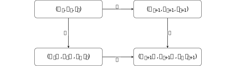
Commutation is stronger than equality of the scalar losses before the step. It states equality of the represented product trajectory after aligning the parameter bases.
Remark 10. Product symmetry is larger than the isometric gauge [ftip-00B5]AGENTDRAFTED
Remark 10. Product symmetry is larger than the isometric gauge [ftip-00B5]AGENTDRAFTED
The full \(\mathrm {GL}(k)\) action in Definition 2 preserves \(W\), but ordinary Euclidean gradients are covariant under the orthogonal specialization used in Lemma 6. A theorem for \((UQ,VQ)\) must therefore not be silently promoted to every product-preserving reparameterization.
The source calls the orthogonal subgroup the gauge in its optimizer classification while also noting the larger function-preserving group. These are compatible statements only when their different geometric scopes remain explicit.