Evaluation, evidence, and finite limits [ftip-00JB]
✍️sourceAGENTDRAFTED
Evaluation, evidence, and finite limits [ftip-00JB]
✍️sourceAGENTDRAFTED
The training and agent mechanisms described earlier produce an artifact whose capability must be evaluated under a declared task law, inference procedure and resource account. This chapter fixes that comparison, studies what survives a change of evaluation, and examines discovery probabilities, support, proxy error and the information available through feedback.
Finite results and counterexamples establish consequences under specific probability laws and computational assumptions. They provide tools for the model-lineage question, where their assumptions must cover an evolving research and training process. The architecture analysis uses the same evaluation framework for comparisons that depend on a model implementation or optimizer.
1. Independent evaluation and post-training potential [ftip-005C]AGENTDRAFTED
1. Independent evaluation and post-training potential [ftip-005C]AGENTDRAFTED
A training score cannot by itself answer how much reliable capability was obtained. This section fixes an evaluation law, an inference procedure, and a resource account before comparing post-training protocols.
Convention 1.1. Fixed evaluation interface for protocol comparison [ftip-005D]AGENTDRAFTED
Convention 1.1. Fixed evaluation interface for protocol comparison [ftip-005D]AGENTDRAFTED
Fix an evaluation task \(\mathsf T_{\rm ev}\) from Definition [ftip-001O] and a measurable scalar evaluation utility \(u_{\mathsf T_{\rm ev}}:\mathcal X_{\mathsf T_{\rm ev}}\times \mathcal O_{\mathsf T_{\rm ev}}\times \Omega _E\to \mathbb R\), the \(d=1\) case of Definition [ftip-001T]. Fix its task law \(Q_{\rm ev}:=\mu _{\mathsf T_{\rm ev}}\), an inference protocol \(\mathsf I_{\rm ev}\) from Definition [ftip-001R], and an inference budget \(b\in \mathcal B_{\mathrm {eval}}\). Use the inference-seed space \(\Omega _I\) and evaluator-seed space \(\Omega _E\) from Notation [ftip-001N]. A declared probability kernel on these measurable spaces \(\Lambda _{\rm ev}(d\xi ,d\omega \mid x)\) assigns inference and evaluator randomness to each instance. Together with \(Q_{\rm ev}\), it gives the joint evaluation law \(\nu _{\rm ev}(dx,d\xi ,d\omega ) =Q_{\rm ev}(dx)\Lambda _{\rm ev}(d\xi ,d\omega \mid x)\), which is fixed independently of training.
Declare a measurable space \(\mathcal M\) of executable artifacts. For \(M\in \mathcal M\), define the aliases \[ \mathsf {Eval}_b(M,x;\xi ) :=\operatorname {pr}_1\left (\mathsf I_{\rm ev}(M,x,b;\xi )\right ), \qquad U(x,o;\omega ):=u_{\mathsf T_{\rm ev}}(x,o;\omega ). \] Require \(\mathsf {Eval}_b\) to be measurable in \((M,x,\xi )\) and to return admissible outcomes on admitted runs.
Each post-training protocol \(P\) has a probability space \((\Omega _P,\Sigma _P,\mathbb P_P)\) for its randomness and a measurable artifact map \(M_P:\Omega _P\to \mathcal M\) produced from the common base artifact \(M_0\). The no-training protocol is \(P_0\). The complete evaluation law for \(P\) is the product \(\mathbb P_P\otimes \nu _{\rm ev}\), expressing independence between protocol randomness and the fixed evaluation draw. For \(\zeta \in \Omega _P\), write \[ Z_P(\zeta ,x,\xi ,\omega ) =U\left (x,\mathsf {Eval}_b(M_P(\zeta ),x;\xi );\omega \right ). \] This composite is measurable. Every protocol compared through expected performance, including the baseline \(P_0\), must satisfy \[ \int |Z_P|\,d(\mathbb P_P\otimes \nu _{\rm ev})<\infty . \] This is the evaluation domain; finite pointwise utility does not replace the absolute-integrability condition. Fix also a scalar success threshold \(u_*\in \mathbb R\).
Definition 1.2. Expected evaluation performance [ftip-005E]AGENTDRAFTED
Definition 1.2. Expected evaluation performance [ftip-005E]AGENTDRAFTED
For a protocol \(P\) in the integrable evaluation domain of Convention 1.1, its expected evaluation performance is the finite real number
\[ \begin {aligned} J_{\rm ev}(P) &=\int Z_P\,d(\mathbb P_P\otimes \nu _{\rm ev}),\\ &=\mathbb E\left [ U\left (X,\mathsf {Eval}_b(M_P,X;\Xi );\Omega \right ) \right ], \\ (X,\Xi ,\Omega )&\sim Q_{\rm ev}(dx)\Lambda _{\rm ev}(d\xi ,d\omega \mid x). \end {aligned} \]The label \(\rm ev\) abbreviates the task, law, inference protocol, budget, utility, and seed law fixed above. Changing any of them changes the estimand. Both positive and negative parts of \(Z_P\) have finite expectation; an undefined expectation or an infinite value is outside this real-valued performance domain.
Definition 1.3. Post-training gain [ftip-005F]AGENTDRAFTED
Definition 1.3. Post-training gain [ftip-005F]AGENTDRAFTED
For \(P\) and the no-training protocol \(P_0\) both satisfying the absolute-integrability condition of Convention 1.1, the post-training gain is the real-valued difference
\[ \Delta J_{\rm ev}(P) =J_{\rm ev}(P)-J_{\rm ev}(P_0). \]Both terms use the same evaluator, task law, utility, and inference budget. The subtraction does not compare different model families or evaluation procedures. In particular, \(+\infty -(+\infty )\) is not an admitted gain.
Remark 1.4. Evaluation gain under a fixed task law [ftip-005G]AGENTDRAFTED
Remark 1.4. Evaluation gain under a fixed task law [ftip-005G]AGENTDRAFTED
The policy-evaluation expectation of Section 3.5 of Reinforcement learning: An introduction[sutton2018reinforcement] specializes to an independently fixed task law and inference procedure. The gain is a paired contrast with the same base artifact and evaluator.
A positive value shows a change under this evaluation. It does not alone show that the trained policy acquired a capability under the criterion of Definition [ftip-0007].
Definition 1.5. Lifecycle cost vector [ftip-005H]AGENTDRAFTED
Definition 1.5. Lifecycle cost vector [ftip-005H]AGENTDRAFTED
The realized lifecycle cost vector of a protocol is the random vector \(C(P)\in \mathbb R_+^7\), measurable on its declared lifecycle-run probability space, that records separately
\[ C(P)= (C_{\rm data},C_{\rm feedback},C_{\rm rollout},C_{\rm env}, C_{\rm update},C_{\rm storage},C_{\rm eval}). \]A componentwise lifecycle budget is a vector \(\mathbf B\in \mathbb R_+^7\). Each cost coordinate has a declared unit, such as tokens, labels, accelerator floating-point operations (FLOPs), sandbox time, bytes, or evaluator calls. A scalar price may be applied later, but the typed vector is retained. Each nonnegative coordinate has a well-defined expectation in \([0,+\infty ]\); finite realized costs need not have finite expectations. A finite componentwise budget excludes protocols with any infinite expected-cost coordinate. When costs include the fixed independent evaluation draw, the run law may include the product law in Convention 1.1; the accounting record must specify which randomness is averaged.
Remark 1.6. Lifecycle costs have distinct units [ftip-005I]AGENTDRAFTED
Remark 1.6. Lifecycle costs have distinct units [ftip-005I]AGENTDRAFTED
The scaling study behind Definition [ftip-001C] reports training tokens and compute separately.
[hoffmann2022training, sec. 3] studies their allocation. Training tokens and compute are therefore separate cost coordinates.
Agentic and replay protocols also incur verifier, environment, storage, and selection work. A training step, a generated rollout, and one second of wall time are therefore different units.
The vector permits later cost models without hiding which conversion rates or hardware assumptions they use.
Definition 1.7. Admissible protocol class [ftip-005J]AGENTDRAFTED
Definition 1.7. Admissible protocol class [ftip-005J]AGENTDRAFTED
For a base artifact \(M_0\), an admissible protocol class \(\mathfrak P(M_0)\) is a declared set of type-correct training procedures. Membership fixes which data sources, feedback channels, model changes, environment interfaces, and update rules are permitted. For the expected performance comparison, every member also satisfies the measurable generation and integrable evaluation domain of Convention 1.1, and carries the measurable nonnegative cost vector of Definition 1.5. The baseline \(P_0\) must satisfy the evaluation domain even if it is not feasible at the chosen cost budget.
The class is part of the research question. Enlarging it can only enlarge the set of attainable outcomes, but may make a comparison less informative.
Definition 1.8. Trust contract [ftip-005K]AGENTDRAFTED
Definition 1.8. Trust contract [ftip-005K]AGENTDRAFTED
A trust contract \(\mathsf {Trust}(P)\) is a predicate requiring the protocol to respect declared provenance, information, and accounting boundaries. At minimum it specifies evaluation independence, behavior-policy stamps for reused rollouts, environment and verifier versions, and complete lifecycle-cost reporting.
The predicate is evidence to be checked. It is not a statement that a protocol is safe, aligned, or free from distribution shift.
Remark 1.9. Allowed procedures and admissible evidence [ftip-005L]AGENTDRAFTED
Remark 1.9. Allowed procedures and admissible evidence [ftip-005L]AGENTDRAFTED
The protocol class and trust contract impose distinct restrictions. The class states what may be attempted; the contract states what evidence an attempt must retain before it can enter the comparison.
Their joint specification is a proposed evaluation framework.
A supremum over an unspecified class or an unaudited evaluation boundary has no stable empirical interpretation.
Definition 1.10. Costed post-training potential [ftip-005M]AGENTDRAFTED
Definition 1.10. Costed post-training potential [ftip-005M]AGENTDRAFTED
For a scalar evaluation utility, the costed post-training potential of \(M_0\) under a finite componentwise budget \(\mathbf B\in \mathbb R_+^7\) is the extended-real supremum
\[ \Phi (M_0,\mathbf B) =\sup _{P\in \mathfrak P(M_0)} \left \{ J_{\rm ev}(P): \mathsf {Trust}(P),\ \mathbb E[C(P)]\leq \mathbf B \right \}. \]Here \(\mathfrak P(M_0)\) has the evaluation domain of Definition 1.7, so each \(J_{\rm ev}(P)\) is real. The expected-cost inequality is componentwise in \([0,+\infty ]^7\); it cannot hold against a finite budget if any coordinate is infinite. Define \(\sup \varnothing =-\infty \), and use \(+\infty \) when feasible performance values are unbounded above. Thus \(\Phi \) takes values in \(\overline {\mathbb R}=\mathbb R\cup \{-\infty ,+\infty \}\).
The potential is finite real exactly when its feasible performance set is nonempty and bounded above. For example, a common finite upper bound on utility and at least one feasible protocol suffice. This does not guarantee that any protocol attains the supremum. Ordinary differences, ratios, or derivatives of potential values require finite real operands and any further regularity hypotheses needed by that operation. The value is conditional on every object named in the display; it is not an intrinsic constant of the model.
Remark 1.11. Potential depends on the intervention and budget [ftip-005N]AGENTDRAFTED
Remark 1.11. Potential depends on the intervention and budget [ftip-005N]AGENTDRAFTED
The potential \(\Phi \) describes how evaluation performance varies with the base artifact, admissible information, protocol family, and resource budget. The definition supplies no scaling exponent and no guarantee that a maximizing protocol exists.
Empirical studies provide conditional points or bounds only after their protocol, evaluator, and costs are embedded in this interface. An observed benchmark maximum need not equal a universal ceiling.
Definition 1.12. feasible objective set [boyd2004convex, Section 4.7.4] [ftip-005O]AGENTDRAFTED
Definition 1.12. feasible objective set [boyd2004convex, Section 4.7.4] [ftip-005O]AGENTDRAFTED
For a multi-objective optimization problem with vector objective \(f(x)\), the feasible objective set is the collection of vectors \(f(x)\) attained by feasible choices \(x\).
In a post-training application, the feasible choice is a trusted, budget-feasible protocol and the objective vector contains independently declared evaluation outcomes.
Definition 1.13. weighted-sum scalarization [boyd2004convex, Section 4.7.5] [ftip-005P]AGENTDRAFTED
Definition 1.13. weighted-sum scalarization [boyd2004convex, Section 4.7.5] [ftip-005P]AGENTDRAFTED
For objective vector \(v\in \mathbb R^m\) and nonnegative weights \(w\in \mathbb R_+^m\), the weighted-sum scalarization assigns the score \(w^\top v\). Optimizing this score selects a point according to the declared weights.
Changing \(w\) changes the research question. A single weighted score can hide tradeoffs among evaluation groups or task families.
Definition 1.14. Pareto-optimal objective vector [boyd2004convex, Section 4.7.4] [ftip-005Q]AGENTDRAFTED
Definition 1.14. Pareto-optimal objective vector [boyd2004convex, Section 4.7.4] [ftip-005Q]AGENTDRAFTED
A feasible vector \(v\) is Pareto optimal when there is no feasible \(v'\) with \(v'_j\geq v_j\) in every coordinate and a strict inequality in at least one coordinate. The Pareto frontier is the set of such vectors.
This order preserves visible tradeoffs. It does not choose one point on the frontier.
Definition 1.15. worst-group risk [sagawa2020distributionally, Section 2] [ftip-005R]AGENTDRAFTED
Definition 1.15. worst-group risk [sagawa2020distributionally, Section 2] [ftip-005R]AGENTDRAFTED
Given predefined groups with risks \(L_g\), the worst-group risk is \(\max _g L_g\). For utilities, the corresponding robust score is \(\min _g J_g\).
A post-training comparison must declare the groups and their evaluation laws before using this score. It is different from an average and from Pareto dominance.
Example 1.16. Three attainable protocols with different scalar, Pareto, and worst-group summaries [ftip-005S]AGENTDRAFTED
Example 1.16. Three attainable protocols with different scalar, Pareto, and worst-group summaries [ftip-005S]AGENTDRAFTED
Three attainable utility vectors separate the answers returned by scalarization, Pareto comparison, and a worst-group summary.
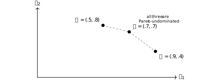
For scalar weights \((0.8,0.2)\), the scores are \(S(A)=0.80\), \(S(B)=0.70\), and \(S(C)=0.56\), so \(A\) wins. The worst-group scores are \(0.4\), \(0.7\), and \(0.5\), so \(B\) wins. No point dominates another coordinatewise, hence the Pareto summary retains all three.
The scalar, Pareto, and worst-group summaries were defined in Definition 1.13--Definition 1.15. Their non-equivalence is explicit in these three points, while the choice of a social or evaluation rule remains open.
2. Evaluation transport and matched protocols [ftip-00F9]AGENTDRAFTED
2. Evaluation transport and matched protocols [ftip-00F9]AGENTDRAFTED
This section compares post-training artifacts only through declared evaluation laws, inference protocols, utilities, seeds, and budgets. It proves finite transport statements locally and treats long-horizon research-state records as empirical evidence, not as theorems.
2.1. Evaluation laws and couplings [ftip-00FA]AGENTDRAFTED
2.1. Evaluation laws and couplings [ftip-00FA]AGENTDRAFTED
Convention 2.1.1. A named evaluation experiment [ftip-00FB]AGENTDRAFTED
Convention 2.1.1. A named evaluation experiment [ftip-00FB]AGENTDRAFTED
A named evaluation experiment records the artifact, task law, inference protocol, evaluator, seed kernel, budget, and sampling unit. Two reported scores are comparable only after these coordinates and their intended target have been stated.
Definition 2.1.2. Evaluation law [ftip-00FC]AGENTDRAFTED
Definition 2.1.2. Evaluation law [ftip-00FC]AGENTDRAFTED
For a fixed evaluation interface from Convention 1.1, an evaluation law is a probability measure \(\mathsf Q\) on the finite outcome space \(\mathcal Z=\mathcal X_{\mathsf T_{\rm ev}}\times \mathcal O_{\mathsf T_{\rm ev}}\) with random pair \((X,O)\sim \mathsf Q\). Its score for artifact \(M\) is a bounded measurable map \(s_M:\mathcal Z\to [0,1]\). Write \(J_{\mathsf Q}(M)=\mathbb E_{\mathsf Q}[s_M(X,O)]\).
Definition 2.1.3. Matched evaluation pair [ftip-00FD]AGENTDRAFTED
Definition 2.1.3. Matched evaluation pair [ftip-00FD]AGENTDRAFTED
A matched evaluation pair is \((\mathsf Q,\mathsf I,b,\Lambda )\) and \((\mathsf Q',\mathsf I',b',\Lambda ')\) together with a coupling \((Z,Z')\) whose marginals are the two laws. The pair is matched on the declared coordinates when the task, utility, evaluator version, and sampling unit are shared; any changed coordinate is named.
Definition 2.1.4. Paired finite score estimator [ftip-00FE]AGENTDRAFTED
Definition 2.1.4. Paired finite score estimator [ftip-00FE]AGENTDRAFTED
For iid coupled draws \((Z_j,Z'_j)_{j=1}^m\), define \(\widehat \Delta _m=m^{-1}\sum _{j=1}^m(s_M(Z_j)-s_{M'}(Z'_j))\). The pairing is part of the estimator specification; it does not silently identify the two evaluation laws.
Theorem 2.1.5. Unbiasedness of the paired score estimator [ftip-00FF]AGENTDRAFTED
Theorem 2.1.5. Unbiasedness of the paired score estimator [ftip-00FF]AGENTDRAFTED
Under the iid coupling in Definition 2.1.4, \(\mathbb E[\widehat \Delta _m]=J_{\mathsf Q}(M)-J_{\mathsf Q'}(M')\).
Proof.
Proof.
Linearity of expectation gives the displayed identity.
\[ \mathbb E[\widehat \Delta _m] =m^{-1}\sum _j\left (\mathbb E[s_M(Z_j)]- \mathbb E[s_{M'}(Z'_j)]\right ). \]The coupling fixes the joint sampling but does not change either marginal, so the two terms are the stated expectations.
Example 2.1.6. Common seeds can reduce paired variance [ftip-00G0]AGENTDRAFTED
Example 2.1.6. Common seeds can reduce paired variance [ftip-00G0]AGENTDRAFTED
If \(s_M(Z)=s_{M'}(Z')\) almost surely under a common-seed coupling, then \(\widehat \Delta _m=0\) for every sample even when independent sampling would have nonzero variance. This is a variance statement, not evidence that the two artifacts have equal behavior on a different law.
Remark 2.1.7. A coupling does not merge estimands [ftip-00G1]AGENTDRAFTED
Remark 2.1.7. A coupling does not merge estimands [ftip-00G1]AGENTDRAFTED
The result in Theorem 2.1.5 follows from its displayed hypotheses. A shared seed can make a paired comparison precise while the changed task law, evaluator, or inference budget still changes the estimand. No causal effect follows without a declared intervention and matched coordinates.
2.2. Utility transport [ftip-00G2]AGENTDRAFTED
2.2. Utility transport [ftip-00G2]AGENTDRAFTED
Definition 2.2.1. Bounded utility perturbation [ftip-00G3]AGENTDRAFTED
Definition 2.2.1. Bounded utility perturbation [ftip-00G3]AGENTDRAFTED
On a common finite outcome law \(\mathsf Q\), let each artifact \(M\) have score maps \(s_M,t_M:\mathcal Z\to [0,1]\). They have perturbation radius \(\varepsilon =\sup _{M,\,z\in \operatorname {supp}(\mathsf Q)} |s_M(z)-t_M(z)|\) when \(0\leq \varepsilon \leq 1\); write \(J_s(M)=\mathbb E_{\mathsf Q}[s_M]\) and \(J_t(M)=\mathbb E_{\mathsf Q}[t_M]\).
Theorem 2.2.2. Direct utility transport bound [ftip-00G4]AGENTDRAFTED
Theorem 2.2.2. Direct utility transport bound [ftip-00G4]AGENTDRAFTED
Under Definition 2.2.1, every artifact \(M\) satisfies \(|J_s(M)-J_t(M)|\leq \varepsilon \).
Proof.
Proof.
Pointwise bounds give \(-\varepsilon \leq s_M(z)-t_M(z)\leq \varepsilon \). Taking expectations preserves both inequalities.
Corollary 2.2.3. Transporting an artifact comparison [ftip-00G5]AGENTDRAFTED
Corollary 2.2.3. Transporting an artifact comparison [ftip-00G5]AGENTDRAFTED
If two artifacts \(M_1,M_0\) are scored by both \(s\) and \(t\) under the same law and \(\lVert s-t\rVert _{\infty ,\mathsf Q}\leq \varepsilon \), then the gain difference obeys \(|(J_s(M_1)-J_s(M_0))-(J_t(M_1)-J_t(M_0))| \leq 2\varepsilon \). This is a finite utility perturbation bound, not a training or distribution-shift theorem.
Example 2.2.4. Equal aggregate score can hide a slice reversal [ftip-00G6]AGENTDRAFTED
Example 2.2.4. Equal aggregate score can hide a slice reversal [ftip-00G6]AGENTDRAFTED
On equally likely outcomes \(a,b\), take score vectors \((s_{M_1}(a),s_{M_1}(b))=(1,0)\) and \((s_{M_0}(a),s_{M_0}(b))=(0,1)\); a second score map swaps coordinates. Both artifacts have aggregate score \(1/2\) under both maps, but their per-outcome ordering reverses. Aggregate transport alone does not identify localized behavior.
Remark 2.2.5. Common domains are a transport hypothesis [ftip-00G7]AGENTDRAFTED
Remark 2.2.5. Common domains are a transport hypothesis [ftip-00G7]AGENTDRAFTED
The bound in Theorem 2.2.2 requires the same finite outcome support. Changing prompts, parsers, evaluators, or inference budgets is a new law and must be recorded rather than hidden inside a score perturbation.
2.3. Prompt and research-state transport [ftip-00G8]AGENTDRAFTED
2.3. Prompt and research-state transport [ftip-00G8]AGENTDRAFTED
Definition 2.3.1. Research-state observable [ftip-00G9]AGENTDRAFTED
Definition 2.3.1. Research-state observable [ftip-00G9]AGENTDRAFTED
For a finite record space \(\mathcal R\), an observable is a map \(h:\mathcal R\to \mathcal H\). A summary-only evaluator sees \(h(r)\) and not the underlying record \(r\); the omitted coordinates are unavailable to that evaluator.
Definition 2.3.2. Compaction kernel [ftip-00GA]AGENTDRAFTED
Definition 2.3.2. Compaction kernel [ftip-00GA]AGENTDRAFTED
A compaction kernel is a randomized map \(K(dh\mid r)\) from records in \(\mathcal R\) to summaries in \(\mathcal H\). A deterministic summary is the special case \(K(dh\mid r)=\delta _{h(r)}\).
Theorem 2.3.3. Summary-only indistinguishability [ftip-00GB]AGENTDRAFTED
Theorem 2.3.3. Summary-only indistinguishability [ftip-00GB]AGENTDRAFTED
Let \(r,r'\in \mathcal R\) induce the same summary law under the kernel in Definition 2.3.2. Any randomized decision rule that receives only that summary has the same output law in the two worlds.
Proof.
Proof.
The output law is the pushforward of the common summary law through the same decision kernel. Pushforwards of equal finite measures are equal.
Example 2.3.4. An omitted feasibility constraint [ftip-00GC]AGENTDRAFTED
Example 2.3.4. An omitted feasibility constraint [ftip-00GC]AGENTDRAFTED
Two research records can share every summary score while one contains a withdrawn lemma and the other contains a feasible proof plan. A summary-only selector therefore chooses identically, although the correct next action differs. This is a finite witness to information loss, not a claim about a particular model.
Remark 2.3.5. Long-horizon records are empirical transport evidence [ftip-00GD]AGENTDRAFTED
Remark 2.3.5. Long-horizon records are empirical transport evidence [ftip-00GD]AGENTDRAFTED
The case study in [li2026longhorizon], Sections 4--7, reports file-based memory, human steering, and research-state failures under one system and task. It motivates explicit observables and omitted constraints; it does not supply the finite theorem in Theorem 2.3.3 or a general model capability law.
2.4. Evaluation cells and budget accounting [ftip-00GE]AGENTDRAFTED
2.4. Evaluation cells and budget accounting [ftip-00GE]AGENTDRAFTED
Definition 2.4.1. Evaluation cell [ftip-00GF]AGENTDRAFTED
Definition 2.4.1. Evaluation cell [ftip-00GF]AGENTDRAFTED
An evaluation cell is \(C=(M,\mathsf Q,\mathsf I,b,\Lambda ,v)\), where \(M\) is an artifact, \(\mathsf Q\) a task law, \(\mathsf I\) an inference protocol, \(b\) a budget, \(\Lambda \) a seed kernel, and \(v\) an evaluator version. A cell comparison may differ in named coordinates only.
Lemma 2.4.2. Additive evaluation cost [ftip-00GG]AGENTDRAFTED
Lemma 2.4.2. Additive evaluation cost [ftip-00GG]AGENTDRAFTED
For a finite evaluation plan with disjoint stages of costs \(c_1,\ldots ,c_k\in \mathbb R_{\geq 0}\), total cost is \(c=\sum _{i=1}^k c_i\). Appending a stage increases cost by its declared amount and cannot preserve a budget \(B\) unless the remaining slack covers it.
Proof.
Proof.
The statement is the associativity and monotonicity of finite sums.
Theorem 2.4.3. Budget-preserving matched comparison [ftip-00GH]AGENTDRAFTED
Theorem 2.4.3. Budget-preserving matched comparison [ftip-00GH]AGENTDRAFTED
Let two evaluation plans use the same declared stages except for a substitution whose cost is at most the replaced stage cost. If their common prefix cost is \(c_0\) and both suffix costs fit \(B-c_0\), then both cells in Definition 2.4.1 are admissible under budget \(B\).
Proof.
Proof.
Apply Lemma 2.4.2 to the common prefix and each suffix. The assumed inequalities give total cost at most \(B\) in each plan.
Example 2.4.4. Cost-balanced evaluation cells [ftip-00GI]AGENTDRAFTED
Example 2.4.4. Cost-balanced evaluation cells [ftip-00GI]AGENTDRAFTED
A paired run can spend \(B=100\) units as 40 units of inference, 20 of evaluator calls, and 40 of audit. Replacing 10 inference units by 10 audit units preserves the budget, but changes the cell and must not be described as the same inference protocol.
Remark 2.4.5. Execution and evaluator confounds [ftip-00GJ]AGENTDRAFTED
Remark 2.4.5. Execution and evaluator confounds [ftip-00GJ]AGENTDRAFTED
A score change can arise from the artifact, prompt law, inference budget, parser, evaluator version, or execution failure. A matched-cell report names these coordinates before interpreting a paired gain.
2.5. Distribution shift and ranking reversals [ftip-00GK]AGENTDRAFTED
2.5. Distribution shift and ranking reversals [ftip-00GK]AGENTDRAFTED
Example 2.5.1. Train and evaluation laws can reverse a ranking [ftip-00GL]AGENTDRAFTED
Example 2.5.1. Train and evaluation laws can reverse a ranking [ftip-00GL]AGENTDRAFTED
Let \(\mathsf Q_{\rm tr}\) put masses \(.9,.1\) on \(a,b\), and let \(\mathsf Q_{\rm ev}\) swap them. Artifacts \(M_1,M_0\) with score vectors \((s_{M_1}(a),s_{M_1}(b))=(1,0)\) and \((s_{M_0}(a),s_{M_0}(b))=(0,1)\) rank oppositely under the two laws. A training score is not an evaluation transport certificate.
Theorem 2.5.2. Total-variation transport bound [ftip-00GM]AGENTDRAFTED
Theorem 2.5.2. Total-variation transport bound [ftip-00GM]AGENTDRAFTED
For any score \(s:\mathcal Z\to [0,1]\) and finite laws \(\mathsf Q,\mathsf Q'\), \(|\mathbb E_{\mathsf Q}s-\mathbb E_{\mathsf Q'}s|\leq \lVert \mathsf Q-\mathsf Q'\rVert _{\rm TV}\), where \(\lVert \mathsf Q-\mathsf Q'\rVert _{\rm TV}:=\frac 12\sum _{z\in \mathcal Z} |\mathsf Q(z)-\mathsf Q'(z)|\).
Proof.
Proof.
Expand the finite expectation difference and use \(|s(z)|\leq 1\). The positive and negative parts are bounded by the total variation mass, giving the displayed inequality.
Example 2.5.3. A sharp two-point transport bound [ftip-00GN]AGENTDRAFTED
Example 2.5.3. A sharp two-point transport bound [ftip-00GN]AGENTDRAFTED
On \(\mathcal Z=\{a,b\}\), let \(s(a)=1,s(b)=0\), and let \(\mathsf Q(a)=1\), \(\mathsf Q'(a)=1-\eta \), and \(\mathsf Q'(b)=\eta \). The score difference and total variation distance are both \(\eta \).
Remark 2.5.4. What transport does not identify [ftip-00GO]AGENTDRAFTED
Remark 2.5.4. What transport does not identify [ftip-00GO]AGENTDRAFTED
The bounds above transport a declared score across a declared law. They do not identify why an artifact changed, establish support expansion, prove generalization, or order different evaluators whose outcome spaces differ.
Example 2.5.5. A minimal evaluation trace [ftip-00GP]AGENTDRAFTED
Example 2.5.5. A minimal evaluation trace [ftip-00GP]AGENTDRAFTED
A reproducible record is \((M,\mathsf Q,\mathsf I,b,\Lambda ,v,m, \widehat \Delta _m,c)\), listing the cells, sample count, paired estimate, and cost. Replaying this tuple reproduces the estimator target only when the recorded laws and versions remain available.
Remark 2.5.6. Execution controls for a matched evaluation [ftip-00GQ]AGENTDRAFTED
Remark 2.5.6. Execution controls for a matched evaluation [ftip-00GQ]AGENTDRAFTED
A matched evaluation requires execution gates, contamination checks, grader calibration, and an audit of the result before it is committed. These controls make the comparison auditable; they do not by themselves establish capability acquisition.
3. Analytical questions and falsifiers [ftip-005T]AGENTDRAFTED
3. Analytical questions and falsifiers [ftip-005T]AGENTDRAFTED
Successful support, verifier error, and entropy statistics distinguish properties that a benchmark summary can combine. Finite examples and counterexamples distinguish these quantities.
Definition 3.1. Successful-support probability [ftip-005U]AGENTDRAFTED
Definition 3.1. Successful-support probability [ftip-005U]AGENTDRAFTED
Fix the evaluation interface and success threshold \(u_*\) from Convention 1.1. For a protocol \(P\) and instance \(x\in \mathcal X_{\mathsf T_{\rm ev}}\), its successful-support probability is
\[ p_P(x) =\Pr \left [ U\left (x,\mathsf {Eval}_b(M_P,x;\Xi );\Omega \right )\geq u_* \right ]. \]The probability includes protocol, inference, environment, and evaluator randomness: \(M_P\) is drawn from the protocol, while \((\Xi ,\Omega )\) is drawn from \(\Lambda _{\rm ev}(\cdot \mid x)\) independently of training. The quantity is instance-specific and budget-specific.
Definition 3.2. Successful-support coverage [ftip-005V]AGENTDRAFTED
Definition 3.2. Successful-support coverage [ftip-005V]AGENTDRAFTED
For threshold \(0<\alpha \leq 1\), the successful-support coverage of protocol \(P\) under evaluation law \(Q_{\rm ev}\) is
\[ \operatorname {Cov}_\alpha (P) =Q_{\rm ev}\left (\{x:p_P(x)\geq \alpha \}\right ). \]Coverage records how much task mass has at least the declared success probability. It does not average the probabilities above or below the threshold.
Remark 3.3. Task-level success and coverage [ftip-005W]AGENTDRAFTED
Remark 3.3. Task-level success and coverage [ftip-005W]AGENTDRAFTED
Increasing probability mass on known solutions need not increase coverage of the task family. Pass-at-\(k\) and related support-sensitive measurements motivate this distinction. Sections 3--5 of Does reinforcement learning really incentivize reasoning capacity in LLMs beyond the base model?[yue2025does] and Sections 2--3 of Understanding r1-zero-like training: A critical perspective[liu2025understanding] compare post-training behavior with base-model support and discuss why response accuracy alone may overstate what RL creates beyond a base model.
The threshold \(\alpha \), inference budget, task law, and success predicate must all be reported. Finite samples estimate this quantity; they do not reveal the unobserved tail without assumptions.
Definition 3.4. Uniform task-family acquisition witness [ftip-005X]AGENTDRAFTED
Definition 3.4. Uniform task-family acquisition witness [ftip-005X]AGENTDRAFTED
Fix a finite, independently selected family \(G\subseteq \mathcal X_{\mathsf T_{\rm ev}}\), thresholds \(0\leq \alpha <\beta \leq 1\), and the common evaluation interface of Convention 1.1. Protocols \(P_0\) and \(P_1\) have a uniform task-family acquisition witness on \(G\) when
\[ p_{P_0}(x)\leq \alpha \quad \hbox {and}\quad p_{P_1}(x)\geq \beta \qquad \text {for every }x\in G. \]For each \(x\), the successful event in Definition 3.1 supplies the fixed-budget transfer event in Definition [ftip-0007]. The displayed inequalities specialize that earlier acquisition witness with \(\varepsilon _0=\alpha \) and \(\varepsilon _1=\beta \), then require the specialization uniformly over \(G\).
Remark 3.5. Acquisition evidence across a fixed task family [ftip-005Y]AGENTDRAFTED
Remark 3.5. Acquisition evidence across a fixed task family [ftip-005Y]AGENTDRAFTED
The proposed family-level criterion is a demanding paired comparison. The task family and evaluator are fixed independently, and both protocols use the same inference budget. It is stronger than one acquisition witness because the threshold change must hold for every member of \(G\).
A theorem may strengthen the witness with confidence bounds, transfer to a predeclared related family, or a lower bound on newly successful support. Each strengthening requires additional sampling or structural assumptions.
Definition 3.6. Verifier error rates [ftip-005Z]AGENTDRAFTED
Definition 3.6. Verifier error rates [ftip-005Z]AGENTDRAFTED
Let \(S\in \{0,1\}\) be an independently defined success label and \(A\in \{0,1\}\) the verifier's accept decision on the same outcome. The false-accept and false-reject rates are
\[ \eta _+=\Pr (A=1\mid S=0), \qquad \eta _-=\Pr (A=0\mid S=1). \]Both rates are conditional on the task and outcome distribution used for the audit. They are undefined when the conditioning event has probability zero.
Remark 3.7. Verifier error under an independent audit law [ftip-0061]AGENTDRAFTED
Remark 3.7. Verifier error under an independent audit law [ftip-0061]AGENTDRAFTED
Verifier error is measured against an independent success label because a training reward cannot audit itself. The verifier and evidence interfaces are in Definition [ftip-0046]--Definition [ftip-0049]. DeepSeek-Prover-V2 [ren2025deepseekproverv2, Section 2.3, ``Reinforcement Learning''] supplies a proof-checking instance. The false-accept/false-reject decomposition is a binary measurement model.
The rates may vary by task, policy, trajectory length, and adversarial pressure. A low average error rate need not prevent reward hacking on the subpopulation favored by optimization.
Example 3.8. Reward hacking under an incomplete checker [ftip-0060]AGENTDRAFTED
Example 3.8. Reward hacking under an incomplete checker [ftip-0060]AGENTDRAFTED
Shifting probability mass toward a checker exploit raises proxy reward while reducing independently judged utility.
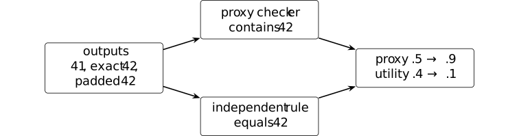
Let the three outputs be \(y_0=\text {41}\), \(y_1=\text {42}\), and \(y_2=\text {ignore; 42; done}\). The proxy accepts \(y_1,y_2\); the independent evaluator accepts only \(y_1\). Moving their probabilities from \((0.5,0.4,0.1)\) to \((0.1,0.1,0.8)\) changes expected proxy reward from \(0.5\) to \(0.9\), but true utility from \(0.4\) to \(0.1\).
Reward exploitation in formal verification is discussed in [ren2025deepseekproverv2, Section 3.2]. The constructed checker exposes one failure mechanism. It provides no basis for treating every executable verifier as incomplete or every proxy improvement as reward hacking.
Definition 3.9. Global policy entropy [ftip-0062]AGENTDRAFTED
Definition 3.9. Global policy entropy [ftip-0062]AGENTDRAFTED
Fix a finite action space, a finite horizon \(T\), and a declared distribution \(\mu _t\) over public histories at each position. The global policy entropy is the weighted average
\[ H_{\rm global}(\pi ) =\frac 1T\sum _{t=0}^{T-1} \mathbb E_{\mathsf H_t\sim \mu _t} \left [-\sum _a\pi (a\mid \mathsf H_t) \log \pi (a\mid \mathsf H_t)\right ]. \]The history distribution and action alphabet are part of the statistic.
We use the convention \(0\log 0=0\) in this and the following position-entropy formula.
Definition 3.10. Token-position entropy [ftip-0063]AGENTDRAFTED
Definition 3.10. Token-position entropy [ftip-0063]AGENTDRAFTED
Let \(T_{\rm tok}\) be the random number of generated tokens. For a one-based token position \(t\) satisfying \(\Pr (T_{\rm tok}\geq t)>0\), condition on \(T_{\rm tok}\geq t\) and let \(\xi _t\) be the token. The token-position entropy is
\[ H_t^{\rm pos} =-\sum _{v\in \mathcal V} \Pr (\xi _t=v\mid T_{\rm tok}\geq t) \log \Pr (\xi _t=v\mid T_{\rm tok}\geq t). \]This is the entropy of a position marginal. It is generally different from the history-conditioned entropy averaged in Definition 3.9.
Definition 3.11. selected-token surprisal [shannon1948mathematical, Part I, Section 6] [ftip-0064]AGENTDRAFTED
Definition 3.11. selected-token surprisal [shannon1948mathematical, Part I, Section 6] [ftip-0064]AGENTDRAFTED
For a sampled token \(\xi _t\) under next-token law \(\pi (\,\cdot \mid \mathsf H_t)\), its surprisal is
\[-\log \pi (\xi _t\mid \mathsf H_t).\]It is a random value attached to the selected token. Its conditional expectation over the token equals the finite Shannon entropy of the next-token law.
Remark 3.12. Why the entropy statistics are not interchangeable [ftip-0065]AGENTDRAFTED
Remark 3.12. Why the entropy statistics are not interchangeable [ftip-0065]AGENTDRAFTED
Shannon's finite entropy A mathematical theory of communication[shannon1948mathematical] can be aggregated over different random objects. Global and position-level entropy statistics use different laws. Selected-token surprisal is a sample statistic, while the other two are expectations under declared history or position laws.
A training intervention can raise one quantity while lowering another. Later claims about exploration or collapse must name the statistic, sampling law, horizon, and conditioning event.
Definition 3.13. empirical squared-ratio excess [miao2026when, Theorem 2] [ftip-0066]AGENTDRAFTED
Definition 3.13. empirical squared-ratio excess [miao2026when, Theorem 2] [ftip-0066]AGENTDRAFTED
For token-level current-to-behavior ratios \(r_1,\ldots ,r_T\), DGG defines
\[\widehat \chi ^2=\frac 1T\sum _{i=1}^T(r_i^2-1).\]The source relates this statistic to an upper bound on language-model-head gradient energy through a batch-dependent constant. In a finite batch \(\widehat \chi ^2\) can be negative, so it is not automatically a nonnegative empirical Pearson divergence. The result also gives no converse from a small batch gradient to small policy shift.
Example 3.14. Lifecycle compute allocation and a finite rollout observation bound [ftip-0067]AGENTDRAFTED
Example 3.14. Lifecycle compute allocation and a finite rollout observation bound [ftip-0067]AGENTDRAFTED
A componentwise lifecycle allocation separates resource accounting from the finite number of rollouts available for observation.
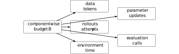
In the coordinate order of Definition 1.5, declare a lifecycle budget vector \(\mathbf B\). Its rollout coordinate permits \(N\) attempts. If each attempt has declared success probability \(p\), then \[ \Pr (\text {at least one success})=1-(1-p)^N\leq Np. \] Only the rollout coordinate enters this calculation; no sum or conversion among heterogeneous coordinates is defined.
The finite bound is the union bound applied to Bernoulli rollouts; finite-horizon success probabilities are standard policy-evaluation objects in [sutton2018reinforcement, Section 3.5]. Independence is needed only for the displayed exact expression. The budget vector is illustrative: neither empirical optimality nor interchangeability of heterogeneous units is inferred from it.
Remark 3.15. Finite questions and necessary assumptions [ftip-0068]AGENTDRAFTED
Remark 3.15. Finite questions and necessary assumptions [ftip-0068]AGENTDRAFTED
Finite analysis raises three questions: how conditional success rates bound long-horizon success, how replay-ratio concentration controls update error, and how trajectory extrapolation with periodic recovery affects evaluation regret. A cost comparison also depends on rollout, update, environment, storage, and evaluation work.
Finite counterexamples show why these questions need additional assumptions. Finite policies can separate the entropy statistics above. Two verifiers can agree on all observed training records yet differ on an unobserved adversarial region. Two parameter paths can share early low-rank summaries and diverge after a new successful rollout. These examples mark where additional assumptions are unavoidable.
The DGG and NExt papers motivate reuse and trajectory-compression hypotheses but do not establish these general results. Bounds on update error and extrapolation regret require assumptions relating the monitored quantities to the corresponding outcomes.
4. Finite consequences and obstructions [ftip-0075]AGENTDRAFTED
4. Finite consequences and obstructions [ftip-0075]AGENTDRAFTED
This section turns parts of the preceding setup into finite mathematical statements. The results concern declared probability spaces, finite decision sets, recorded feedback, or explicitly stated matrix models. They do not by themselves establish a scaling law for language-model capability.
We begin with discovery and support, then study proxy rewards and verifiers. The third subsection asks what can be learned from a fixed feedback transcript. The last subsection studies the DGG inequalities before introducing trajectory-compression diagnostics and counterexamples.
4.1. Finite discovery and support [ftip-0076]AGENTDRAFTED
4.1. Finite discovery and support [ftip-0076]AGENTDRAFTED
A successful continuation can have positive probability and still be difficult to observe within a finite rollout budget. This subsection separates the probability of observing a success from support, coverage, and capability acquisition.
Convention 4.1.1. Repeated attempts and the discovery event [ftip-0077]AGENTDRAFTED
Convention 4.1.1. Repeated attempts and the discovery event [ftip-0077]AGENTDRAFTED
Fix a task instance, evaluator, success threshold, and a joint law for \(B\geq 1\) attempts. Let \(E_i\) be the event that attempt \(i\) succeeds. The discovery event by attempt \(B\) is
\[ D_B=\bigcup _{i=1}^{B}E_i. \]Write \(p_i=\Pr (E_i)\). Independence is an additional property of the declared joint law; it is not implied by repeated decoding, a shared model, or a common environment. In the independent and identically distributed case, write \(p_i=p\). When the attempt law is the one fixed in Definition 3.1, this \(p\) is the corresponding successful-support probability.
Theorem 4.1.2. Discovery under independent attempts [ftip-0078]AGENTDRAFTED
Theorem 4.1.2. Discovery under independent attempts [ftip-0078]AGENTDRAFTED
Assume the events \(E_1,\ldots ,E_B\) of Convention 4.1.1 are independent. Then
\[ \Pr (D_B)=1-\prod _{i=1}^{B}(1-p_i). \]In particular, independent attempts with a common success probability \(p\) satisfy
\[ \Pr (D_B)=1-(1-p)^B. \]
Proof.
Proof.
The complement of discovery is \(D_B^{\mathsf c}=\bigcap _{i=1}^{B}E_i^{\mathsf c}\). Independence gives \(\Pr (D_B^{\mathsf c})=\prod _i\Pr (E_i^{\mathsf c}) =\prod _i(1-p_i)\). Taking complements proves the first identity; substituting \(p_i=p\) proves the specialization.
This finite statement follows from the displayed hypotheses. The calculation in Example 3.14 is its ten-attempt numerical preview.
Corollary 4.1.3. A rollout budget for target discovery probability [ftip-0079]AGENTDRAFTED
Corollary 4.1.3. A rollout budget for target discovery probability [ftip-0079]AGENTDRAFTED
This is a finite corollary of Theorem 4.1.2, obtained from its displayed hypotheses.
Let \(0<\delta <1\). Under the independent and identically distributed setup of Theorem 4.1.2, suppose first that \(0<p<1\). The least positive integer budget whose discovery failure probability is at most \(\delta \) is
\[ B_{\min } =\left \lceil \frac {\log \delta }{\log (1-p)}\right \rceil . \]If \(p=0\), no finite positive budget reaches failure probability below one. If \(p=1\), one attempt suffices.
Proof.
Proof.
For \(0<p<1\), Theorem 4.1.2 gives failure probability \((1-p)^B\). The inequality \((1-p)^B\leq \delta \) is equivalent to \(B\geq \frac {\log \delta }{\log (1-p)}\) because both logarithms are negative. The least integer solution is the displayed ceiling. The two boundary cases follow directly from \((1-p)^B\).
Lemma 4.1.4. Discovery bounds from conditional success rates [ftip-007A]AGENTDRAFTED
Lemma 4.1.4. Discovery bounds from conditional success rates [ftip-007A]AGENTDRAFTED
Put \(D_0=\varnothing \). Whenever \(\Pr (D_{i-1}^{\mathsf c})>0\), define the surviving conditional success rate
\[ q_i=\Pr (E_i\mid D_{i-1}^{\mathsf c}). \]If these rates are defined through step \(B\), then
\[ \Pr (D_B^{\mathsf c})=\prod _{i=1}^{B}(1-q_i). \]Consequently, if \(0\leq \underline q\leq q_i\leq \overline q\leq 1\) for every surviving step, then
\[ 1-(1-\underline q)^B \leq \Pr (D_B) \leq 1-(1-\overline q)^B. \]
Proof.
Proof.
The chain rule gives \(\Pr (D_i^{\mathsf c})=\Pr (D_{i-1}^{\mathsf c})(1-q_i)\). Iteration proves the product identity, and the coordinatewise bounds on \(1-q_i\) give the two discovery bounds.
No independence assumption is used. The conditional rates may change with the earlier failures, an adaptive decoder, or a changing environment state.
This finite statement follows from the displayed hypotheses.
Remark 4.1.5. Discovery is neither acquisition nor coverage [ftip-007B]AGENTDRAFTED
Remark 4.1.5. Discovery is neither acquisition nor coverage [ftip-007B]AGENTDRAFTED
The discovery event concerns whether a declared sampling procedure observes at least one success. Increasing its probability can be an elicitation effect in the sense of Definition [ftip-0005]: more attempts expose behaviour that already had positive probability. It is not by itself the independent before--after comparison required by Definition [ftip-0007].
Successful-support coverage in Definition 3.2 integrates an instance-level threshold over a task law. A large discovery probability on one instance therefore does not establish broad coverage or the uniform task-family witness of Definition 3.4.
Theorem 4.1.6. Finite exponential tilting preserves support [ftip-007C]AGENTDRAFTED
Theorem 4.1.6. Finite exponential tilting preserves support [ftip-007C]AGENTDRAFTED
Fix a prompt \(x\), a finite response set \(\mathcal Y\), a reference policy \(\pi _{\mathrm {ref}}\), a finite real reward \(r(x,y)\), and \(\beta >0\). Let \(\pi _r\) be the normalized exponential tilt of Definition [ftip-003O]. Then, for every \(y\in \mathcal Y\),
\[ \pi _r(y\mid x)>0 \quad \Longleftrightarrow \quad \pi _{\mathrm {ref}}(y\mid x)>0. \]
Proof.
Proof.
The multiplier \(\exp (r(x,y)/\beta )\) is finite and strictly positive. The finite normalizer \(Z_r(x)\) is also strictly positive. Multiplication by the first quantity and division by the second therefore preserve whether the reference mass is zero or positive.
The source policy form appears as equation (4) in [rafailov2023direct, Section 4]; the displayed result is the finite corollary derived here. Infinite rewards, non-normalizable response spaces, approximate optimization, and changes to the generation mechanism lie outside the statement.
Remark 4.1.7. Formal support and operational discoverability [ftip-007D]AGENTDRAFTED
Remark 4.1.7. Formal support and operational discoverability [ftip-007D]AGENTDRAFTED
Support preservation is a statement about exact positive probability. A response can remain in mathematical support while its mass becomes too small to observe within the available rollout budget. The identities in Theorem 4.1.2 and Corollary 4.1.3 quantify this distinction for declared independent attempts.
Top-\(k\) truncation, nucleus sampling, finite numerical precision, context limits, and parser constraints can also remove an operational route even when the underlying softmax law assigns it positive mass. Claims about elicitation must therefore name both the policy law and the executable inference procedure.
Example 4.1.8. Counterexample: Equal one-shot success, unequal successful coverage [ftip-007E]AGENTDRAFTED
Example 4.1.8. Counterexample: Equal one-shot success, unequal successful coverage [ftip-007E]AGENTDRAFTED
Let the evaluation law be uniform on two instances \(x_1,x_2\). Consider protocols \(P\) and \(P'\) with successful-support probabilities
\[ \bigl (p_P(x_1),p_P(x_2)\bigr ) =\left (\frac 12,\frac 12\right ), \qquad \bigl (p_{P'}(x_1),p_{P'}(x_2)\bigr ) =(1,0). \]Both protocols have mean one-shot success \(1/2\). At threshold \(\alpha =1/2\), however, Definition 3.2 gives
\[ \operatorname {Cov}_{1/2}(P)=1, \qquad \operatorname {Cov}_{1/2}(P')=\frac 12. \]Thus average success does not determine successful-support coverage. The example is finite and uses the same task law and threshold for both protocols; it does not compare their training costs or establish acquisition.
4.2. Proxy reward and verifier fidelity [ftip-007F]AGENTDRAFTED
4.2. Proxy reward and verifier fidelity [ftip-007F]AGENTDRAFTED
A proxy can guide an update or rank sampled candidates without agreeing with the independently declared utility of the resulting output. This subsection separates pointwise proxy error from average error under a shifted law. It then distinguishes repeated false-accept events from the output of a candidate selector. Pointwise approximation and explicit probability assumptions support different guarantees; an average audit number alone supplies neither.
Definition 4.2.1. Uniform proxy approximation [ftip-007G]AGENTDRAFTED
Definition 4.2.1. Uniform proxy approximation [ftip-007G]AGENTDRAFTED
Let \(\mathcal Y_0\) be a nonempty finite set of candidate outcomes. Let \(U:\mathcal Y_0\to \mathbb R\) be an independently declared utility and \(\widehat U:\mathcal Y_0\to \mathbb R\) a proxy score. The proxy is a uniform approximation to \(U\) on \(\mathcal Y_0\) with error \(\varepsilon \) when \(\varepsilon \geq 0\) and
\[ \sup _{y\in \mathcal Y_0}\lvert \widehat U(y)-U(y)\rvert \leq \varepsilon . \]The candidate set is part of the claim. Approximation on training outcomes, on one policy's support, or in expectation is not uniform approximation on a larger set reached after optimization.
Theorem 4.2.2. Uniform proxy error gives two-epsilon selection regret [ftip-007H]AGENTDRAFTED
Theorem 4.2.2. Uniform proxy error gives two-epsilon selection regret [ftip-007H]AGENTDRAFTED
Under the conditions of Definition 4.2.1, choose
\[ y^\star \in \operatorname *{arg\,max}_{y\in \mathcal Y_0}U(y), \qquad \widehat y\in \operatorname *{arg\,max}_{y\in \mathcal Y_0}\widehat U(y). \]Then the utility regret of selecting by the proxy satisfies
\[ 0\leq U(y^\star )-U(\widehat y)\leq 2\varepsilon . \]
Proof.
Proof.
Optimality of \(\widehat y\) for the proxy and the two pointwise error bounds give
\[ \begin {aligned} U(y^\star ) &\leq \widehat U(y^\star )+\varepsilon \\ &\leq \widehat U(\widehat y)+\varepsilon \\ &\leq U(\widehat y)+2\varepsilon . \end {aligned} \]Optimality of \(y^\star \) for \(U\) gives the lower bound.
This finite statement follows from the displayed hypotheses.
Remark 4.2.3. The two-epsilon theorem is a decision bound [ftip-007I]AGENTDRAFTED
Remark 4.2.3. The two-epsilon theorem is a decision bound [ftip-007I]AGENTDRAFTED
The bound in Theorem 4.2.2 follows directly from the uniform approximation condition. It compares two maximizers on one fixed finite candidate set. It does not describe how either score was learned or how a policy changes when that score becomes a training objective.
The result is useful because its transfer assumption is visible. To apply it after an update or a larger search, the uniform bound must hold on the outcomes that the new procedure can actually select. The verifier evidence of Definition [ftip-0047] can support such an audit, but reproducible evidence alone does not establish the bound.
Example 4.2.4. Counterexample: Small average proxy error fails after distribution shift [ftip-007J]AGENTDRAFTED
Example 4.2.4. Counterexample: Small average proxy error fails after distribution shift [ftip-007J]AGENTDRAFTED
Let the finite decision set be \(\mathcal Y_0=\{y_{\rm safe},y_{\rm exploit}\}\). Define its utility and proxy utility by the following table.
\[ \begin {array}{c|cc} &y_{\rm safe}&y_{\rm exploit}\\ \hline U&1&0\\ \widehat U&1&2. \end {array} \]For \(0<\delta <1\), let a reference law \(P_\delta \) assign probability \(\delta \) to \(y_{\rm exploit}\). Its mean absolute proxy error is
\[ \mathbb E_{P_\delta }\lvert \widehat U-U\rvert =2\delta , \]which tends to zero with \(\delta \). Nevertheless, proxy maximization selects \(y_{\rm exploit}\) and incurs utility regret \(1\). Under the shifted law concentrated on that selected outcome, the mean error is \(2\). Thus no vanishing selection-regret bound can depend only on average error under the reference law.
This two-outcome construction isolates the distribution-shift warning in Remark 3.7. It does not claim that a particular learned verifier has this error profile; Example 3.8 gives a source-linked checker instance with the same proxy-versus-utility separation.
Definition 4.2.5. Repeated verifier audit [ftip-007K]AGENTDRAFTED
Definition 4.2.5. Repeated verifier audit [ftip-007K]AGENTDRAFTED
A repeated verifier audit of size \(N\geq 1\) records pairs \((S_i,A_i)\in \{0,1\}^2\) for candidates \(1\leq i\leq N\). Here \(S_i\) is an independently defined success label and \(A_i\) is the verifier decision, as in Definition 3.6. Define
\[ C_i^{\rm fa}=\{S_i=0,\ A_i=1\}, \qquad \mathcal E_N^{\rm fa}=\bigcup _{i=1}^N C_i^{\rm fa}. \]The event \(\mathcal E_N^{\rm fa}\) says that at least one invalid candidate was accepted. It does not say which candidate a downstream selector returns. Write \(\phi _i=\Pr (C_i^{\rm fa})\). When \(\iota _i=\Pr (S_i=0)>0\), the conditional false-accept rate \(\eta _{+,i}=\Pr (A_i=1\mid S_i=0)\) is defined and \(\phi _i=\iota _i\eta _{+,i}\).
Theorem 4.2.6. Independent false accepts amplify with candidate count [ftip-007L]AGENTDRAFTED
Theorem 4.2.6. Independent false accepts amplify with candidate count [ftip-007L]AGENTDRAFTED
In the repeated audit of Definition 4.2.5, suppose the pairs \((S_i,A_i)\) are independent and identically distributed. Assume
\[ \iota =\Pr (S_i=0)>0, \qquad \eta _+=\Pr (A_i=1\mid S_i=0). \]Then the probability that at least one accepted invalid candidate exists among the \(N\) audited candidates is
\[ \Pr (\mathcal E_N^{\rm fa})=1-(1-\iota \eta _+)^N. \]It is strictly increasing in \(N\) when \(0<\iota \eta _+<1\), and it converges to \(1\) when \(\iota \eta _+>0\).
Proof.
Proof.
Each \(C_i^{\rm fa}\) has probability \(\iota \eta _+\). Independence of the audited pairs makes the events \(C_i^{\rm fa}\) independent. Therefore
\[ \Pr \left ((\mathcal E_N^{\rm fa})^c\right ) =\Pr \left (\bigcap _{i=1}^N (C_i^{\rm fa})^c\right ) =\prod _{i=1}^N(1-\iota \eta _+) =(1-\iota \eta _+)^N. \]Taking complements gives the equality. The monotonicity and limit follow from the elementary powers of \(1-\iota \eta _+\).
This finite statement follows from the displayed hypotheses.
Theorem 4.2.7. A false-accept union bound without independence [ftip-007M]AGENTDRAFTED
Theorem 4.2.7. A false-accept union bound without independence [ftip-007M]AGENTDRAFTED
For any joint law of a repeated verifier audit,
\[ \Pr (\mathcal E_N^{\rm fa})\leq \sum _{i=1}^N \phi _i. \]If \(\iota _i=\Pr (S_i=0)>0\) for every \(i\), this becomes
\[ \Pr (\mathcal E_N^{\rm fa})\leq \sum _{i=1}^N \iota _i\eta _{+,i}. \]
Proof.
Proof.
Apply the union bound to \(\mathcal E_N^{\rm fa}=\bigcup _i C_i^{\rm fa}\). The factorization \(\phi _i=\iota _i\eta _{+,i}\) follows from conditional probability whenever \(\iota _i>0\). If \(\iota _i=0\), then \(\phi _i=0\) while the corresponding conditional rate is undefined, so the first display remains the unconditional statement.
Without a dependence assumption, matching marginal error rates do not give the equality in Theorem 4.2.6; the events \(C_i^{\rm fa}\) could coincide.
This finite statement follows from the displayed hypotheses.
Example 4.2.8. Weight updates and candidate selection are different proxy operators [ftip-007N]AGENTDRAFTED
Example 4.2.8. Weight updates and candidate selection are different proxy operators [ftip-007N]AGENTDRAFTED
A proxy score can enter a training operator or a selection operator. In the first route it changes the policy; in the second it ranks a finite sample from a policy whose weights remain fixed.
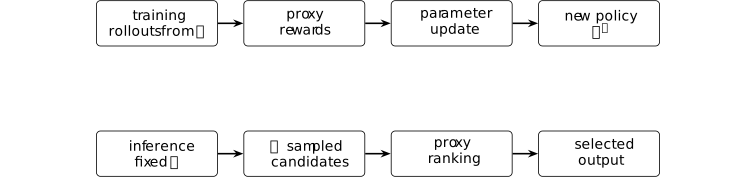
The lifecycle accounting of Definition 1.5 places the first route's rollout and update work in separate coordinates. The second route incurs rollout and evaluation work but no parameter update. Consequently, the event \(\mathcal E_N^{\rm fa}\) in Definition 4.2.5 concerns the candidate set presented to selection; it is not a claim about the selected output or a training-time policy change.
Remark 4.2.9. What verifier error rates do not identify [ftip-007O]AGENTDRAFTED
Remark 4.2.9. What verifier error rates do not identify [ftip-007O]AGENTDRAFTED
The rates in Definition 3.6 are properties of a declared audit law. They do not identify where errors occur within the task family, how error events depend across repeated candidates, or which accepted candidate a selector returns. Theorem 4.2.6 adds identical marginals and independence; Theorem 4.2.7 retains only the union bound.
Nor do these rates determine the effect of optimizing against the verifier. That effect depends on how the induced policy or selection law moves mass toward particular outcomes. The incomplete-checker example Example 3.8 demonstrates one such movement, while Example 4.2.4 shows why an average reference-law error cannot rule it out. These are local finite statements. Any claim about a named verifier still requires its own audit distribution, evidence, and transfer argument.
The deterministic regret lemma Theorem 4.2.2, the independent-audit identity Theorem 4.2.6, and the union bound Theorem 4.2.7 follow from uniform approximation, independent trials, and subadditivity, respectively. Their hypotheses need not hold for a verifier chosen only for its empirical performance.
4.3. Feedback identifiability and fixed records [ftip-007P]AGENTDRAFTED
4.3. Feedback identifiability and fixed records [ftip-007P]AGENTDRAFTED
A training protocol can respond only to distinctions present in its observations. The following finite setup makes that restriction precise before considering stronger, model-specific limits on preference data.
Definition 4.3.1. Finite declared feedback protocol [ftip-007Q]AGENTDRAFTED
Definition 4.3.1. Finite declared feedback protocol [ftip-007Q]AGENTDRAFTED
Fix a horizon \(N\geq 0\), finite action sets \(\mathcal A_n\), finite feedback sets \(\mathcal F_n\), and a finite internal-seed set \(\mathcal U\) with a declared law \(\lambda \). A finite declared protocol \(\mathsf P\) consists of selection maps
\[ a_n:\mathcal U\times \prod _{j<n}(\mathcal A_j\times \mathcal F_j) \longrightarrow \mathcal A_n \qquad (0\leq n<N). \]An action may specify the task, rollout record, feedback request, or sampling choice made at that round. The protocol can depend on earlier exposed feedback and its declared seed, but it cannot depend on a latent world field that has not entered those arguments.
Definition 4.3.2. Finite feedback world [ftip-008C]AGENTDRAFTED
Definition 4.3.2. Finite feedback world [ftip-008C]AGENTDRAFTED
For the action and feedback sets of Definition 4.3.1, a finite feedback world \(w\) supplies, for each round \(0\leq n<N\), a probability kernel \(K_{n,w}\) from a generic action--feedback history \((a_0,f_0,\ldots ,a_n)\) ending in \(a_n\in \mathcal A_n\) to \(\mathcal F_n\). Thus, whenever \(a_j\in \mathcal A_j\) and \(f_j\in \mathcal F_j\),
\[ K_{n,w}(\,\cdot \mid a_0,f_0,\ldots ,a_n) \in \Delta (\mathcal F_n). \]Two worlds may agree on every feedback kernel queried by a protocol while differing in latent utility, unrequested labels, or unobserved environment facts. Those latent fields are not feedback until a declared query exposes them.
Definition 4.3.3. Observed feedback transcript [ftip-008D]AGENTDRAFTED
Definition 4.3.3. Observed feedback transcript [ftip-008D]AGENTDRAFTED
Fix a finite declared protocol \(\mathsf P\) from Definition 4.3.1 and a finite feedback world \(w\) from Definition 4.3.2. Draw \(U\sim \lambda \) and, for \(0\leq n<N\), set
\[ \begin {aligned} A_n&=a_n(U,A_0,F_0,\ldots ,A_{n-1},F_{n-1}),\\ F_n&\sim K_{n,w}(\,\cdot \mid A_0,F_0,\ldots ,A_n). \end {aligned} \]The resulting observed feedback transcript is
\[ T_w^{\mathsf P}=(U,A_0,F_0,\ldots ,A_{N-1},F_{N-1}). \]All protocol randomness is included in \(U\). Immutable rollout records and typed feedback events may be components of the finite action and feedback sets, as in Definition [ftip-0051] and Definition [ftip-0053].
Definition 4.3.4. Observational equivalence for a declared protocol [ftip-007R]AGENTDRAFTED
Definition 4.3.4. Observational equivalence for a declared protocol [ftip-007R]AGENTDRAFTED
Let \(\mathcal T_{\mathsf P}\) be the finite set of possible transcripts for a declared protocol \(\mathsf P\). Two feedback worlds \(w_0,w_1\) are observationally equivalent for \(\mathsf P\), written \(w_0\equiv _{\mathsf P}w_1\), when
\[ \Pr (T_{w_0}^{\mathsf P}=t)=\Pr (T_{w_1}^{\mathsf P}=t) \qquad \text {for every }t\in \mathcal T_{\mathsf P}. \]The relation is protocol-relative. Another protocol may issue a different feedback request and thereby separate the same worlds. Equality only on the realized transcript is weaker than this definition, which compares the whole finite transcript law.
Theorem 4.3.5. Post-training cannot distinguish observationally equivalent worlds [ftip-007S]AGENTDRAFTED
Theorem 4.3.5. Post-training cannot distinguish observationally equivalent worlds [ftip-007S]AGENTDRAFTED
For a finite random variable \(X\), write \(\operatorname {Law}(X)\) for its probability law. If \(h\) maps the value space of \(X\) to a finite set \(\mathcal Y\), its pushforward law \(h_{\#}\operatorname {Law}(X)\) is characterized by \[ \bigl (h_{\#}\operatorname {Law}(X)\bigr )(\{y\}) =\Pr (h(X)=y),\qquad y\in \mathcal Y. \]
Let \(w_0\equiv _{\mathsf P}w_1\). For any finite output set \(\mathcal Y\) and any readout \(h:\mathcal T_{\mathsf P}\to \mathcal Y\),
\[ h_{\#}\operatorname {Law}(T_{w_0}^{\mathsf P}) =h_{\#}\operatorname {Law}(T_{w_1}^{\mathsf P}). \]Thus a final artifact stamp, update decision, or test chosen solely from the declared protocol's transcript has the same distribution in both worlds.
Proof.
Proof.
For every \(y\in \mathcal Y\), finiteness gives
\[ \begin {aligned} \Pr \left (h(T_{w_0}^{\mathsf P})=y\right ) &=\sum _{\substack {t\in \mathcal T_{\mathsf P}\\h(t)=y}} \Pr (T_{w_0}^{\mathsf P}=t)\\ &=\sum _{\substack {t\in \mathcal T_{\mathsf P}\\h(t)=y}} \Pr (T_{w_1}^{\mathsf P}=t) =\Pr \left (h(T_{w_1}^{\mathsf P})=y\right ). \end {aligned} \]The middle equality is observational equivalence from Definition 4.3.4. These point probabilities determine the two pushforward laws.
This finite statement follows from the displayed hypotheses.
Remark 4.3.6. A no-free-feedback result, not a no-learning result [ftip-007T]AGENTDRAFTED
Remark 4.3.6. A no-free-feedback result, not a no-learning result [ftip-007T]AGENTDRAFTED
Theorem 4.3.5 says that the declared observations supply no information that distinguishes \(w_0\) from \(w_1\). It does not say that the output must equal the initial model, that the parameters cannot change, or that performance cannot improve in both worlds. Pretraining, inductive bias, computation on the observed records, and generalization may still produce an improvement shared by the two worlds.
Calling the theorem a no-learning result would therefore erase the central condition: only world-dependent conclusions unavailable from the common transcript are ruled out.
Corollary 4.3.7. Replaying a fixed pool supplies no new feedback information [ftip-007U]AGENTDRAFTED
Corollary 4.3.7. Replaying a fixed pool supplies no new feedback information [ftip-007U]AGENTDRAFTED
Fix a realized finite replay pool \(d\) as in Definition [ftip-0056]. Let \(\mathcal V\) be a finite seed set, and let \(V\in \mathcal V\) be a replay-and-update seed with the same declared law in two feedback worlds and whose law does not depend on the world. If a replay-only procedure makes no new environment or feedback query, then its output has the form \(Y=h(d,V)\). The law of \(Y\) is the same in the two worlds.
Proof.
Proof.
For every output \(y\),
\[ \Pr (h(d,V)=y)= \sum _{\substack {v\in \mathcal V\\h(d,v)=y}}\Pr (V=v). \]The fixed pool, seed law, and readout are identical in the two worlds, so the displayed sum is identical. Equivalently, this is the pushforward argument of Theorem 4.3.5 applied after conditioning on the realized pool.
This finite statement follows from the displayed hypotheses.
Remark 4.3.8. Reuse can change optimization without enlarging evidence [ftip-007V]AGENTDRAFTED
Remark 4.3.8. Reuse can change optimization without enlarging evidence [ftip-007V]AGENTDRAFTED
A replay schedule can reweight records, reduce optimization error on the fixed pool, or produce a different update proposal in the sense of Definition [ftip-006C]. Those are genuine computational effects. They do not add a label, preference, verifier result, or environment transition to the fixed evidence. Fresh optimizer randomness is likewise not feedback about the latent world.
This distinction prevents sample reuse from being counted as feedback acquisition. It does not imply that replay is useless; it isolates the source of any benefit as further computation on already acquired records.
Example 4.3.9. Counterexample: An off-query utility reversal [ftip-007W]AGENTDRAFTED
Example 4.3.9. Counterexample: An off-query utility reversal [ftip-007W]AGENTDRAFTED
Let the response set be \(\{a,b\}\). A one-round protocol queries only \(x_0\); both worlds return the preference \(a\succ b\). The protocol therefore has the same transcript law in both worlds. Fix a deterministic transcript-to-policy readout that chooses \(a\) also at an unqueried \(x_1\). The worlds agree on every observed field but reverse utility at \(x_1\):
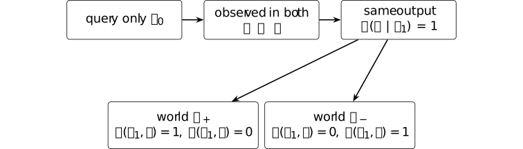
The transcript laws are identical, so Theorem 4.3.5 applies, while the deterministic readout returns the same output in both worlds. That output is optimal in \(w_+\) and suboptimal in \(w_-\) on \(x_1\). The example does not show that generalization always fails. It shows that a claim about unqueried utility requires an assumption connecting observed feedback to that utility.
Remark 4.3.10. From finite indistinguishability to preference-data limits [ftip-007X]AGENTDRAFTED
Remark 4.3.10. From finite indistinguishability to preference-data limits [ftip-007X]AGENTDRAFTED
[zhao2025limits, Theorems 3.3--3.5] study a more structured post-training model. They give ordinal-preference distortion lower bounds, including a lower bound under Bradley--Terry noise with linear scores, and a positive result using a limited number of cardinal queries. These results depend on the routing model, utility class, and query budget developed in § 5.2.
Theorem 4.3.5 gives a finite pushforward theorem, while Example 4.3.9 gives a counterexample to identification from an incomplete transcript. They are neither proofs nor special cases of the paper's distortion results.
4.4. Replay monitors and trajectory compression [ftip-007Y]AGENTDRAFTED
4.4. Replay monitors and trajectory compression [ftip-007Y]AGENTDRAFTED
Reusing a rollout and jumping along a predicted checkpoint path save different kinds of work. The first changes how often recorded feedback enters an update. The second replaces some realized training steps by a parameter forecast. This subsection records what their proposed monitors establish and, separately, what remains unmeasured.
Theorem 4.4.1. DGG head gradient and shared-weight occurrence sum [ftip-007Z]AGENTDRAFTED
Theorem 4.4.1. DGG head gradient and shared-weight occurrence sum [ftip-007Z]AGENTDRAFTED
Fix a sampled history and an active token \(i\) in the interior of the unclipped branch of the GRPO objective. Consider a finite directed acyclic computation graph that is differentiable at the parameter point in question. Let \(a_i\) be the sampled token, \(\widehat A_i\) its fixed normalized advantage, and \(p_i=\operatorname {softmax}(z_i)\) the current distribution on a finite vocabulary \(\mathcal V\). With fixed behavior probability \(b_i>0\), set \[ r_i=\frac {p_i(a_i)}{b_i}, \qquad \mathcal L_i=r_i\widehat A_i, \qquad E_i=r_i\widehat A_i(e_{a_i}-p_i). \] Here \(e_{a_i}\in \mathbb R^{|\mathcal V|}\) is the sampled-token basis vector. The history and sampling decisions are held fixed during differentiation.
Suppose the output head \(W_{\rm lm}\in \mathbb R^{|\mathcal V|\times d_{\rm model}}\) is untied: its only path to \(\mathcal L_i\) is through \(z_i=W_{\rm lm}h_{L,i}\), and \(h_{L,i}\in \mathbb R^{d_{\rm model}}\) is independent of \(W_{\rm lm}\). Then \[ G_i^{\rm lm}=\nabla _{W_{\rm lm}}\mathcal L_i =E_i h_{L,i}^{\mathsf T}. \]
Let \(W_{\rm int}\in \mathbb R^{m\times d}\) be a shared intermediate weight. Index by a finite set \(\mathcal O_i\) every occurrence of this weight that can affect \(z_i\), assuming that all such uses have the form \(y_o=W_{\rm int}x_o\), with \(x_o\in \mathbb R^d\). First replace these uses by independent copies \(W_o\) and evaluate them all at \(W_o=W_{\rm int}\). Let \(J_{io}\in \mathbb R^{|\mathcal V|\times m}\) be the downstream Jacobian from node \(y_o\) to \(z_i\) in this graph, with the other weight copies fixed. Define the contribution of occurrence \(o\) by \[ H_{io}=\nabla _{W_o}\mathcal L_i =(J_{io}^{\mathsf T}E_i)x_o^{\mathsf T}. \] On tying the copies, the total derivative is \[ G_i^{\rm int}=\nabla _{W_{\rm int}}\mathcal L_i =\sum _{o\in \mathcal O_i}H_{io}. \] The head gradient and each occurrence contribution have rank at most one; the total shared-weight gradient need not.
For a layer used once per position in a causal network, the sum includes every earlier position whose output affects token \(i\). Reuse across depth adds further occurrences. Tying the head to embeddings or other blocks also requires their contributions; the displayed head identity assumes that such tying is absent.
Proof.
Proof.
Softmax differentiation gives \(\nabla _{z_i}\mathcal L_i=E_i\). The outer-product rule gives the untied head identity. In the graph with independent copies, \(x_o\) does not depend on its own \(W_o\); all downstream paths from \(y_o\) are included in \(J_{io}\). The chain rule therefore gives \(\nabla _{W_o}\mathcal L_i=(J_{io}^{\mathsf T}E_i)x_o^{\mathsf T}\). Finally, the derivative of the diagonal map \(W_{\rm int}\mapsto (W_o=W_{\rm int})_{o\in \mathcal O_i}\) adds these partial derivatives.
Clipped or inactive terms require their own derivative or mask. [miao2026when, Section 4.2.1, Proposition 1, and Appendix A.1] derives the intermediate outer product through one local application. For a shared weight, that calculation gives \(H_{io}\); identifying it with the total \(G_i^{\rm int}\) omits the other occurrences. The sum above supplies the chain rule needed for shared parameters.
Theorem 4.4.2. DGG occurrence-to-head gradient-energy bound [ftip-0080]AGENTDRAFTED
Theorem 4.4.2. DGG occurrence-to-head gradient-energy bound [ftip-0080]AGENTDRAFTED
Use the per-token quantities and untied head of Theorem 4.4.1, and fix one occurrence \(o\in \mathcal O_i\). Assume \(d_{\rm model}\geq 1\) and positive constants \(\alpha _{\min }\), \(\beta _{\max }\), and \(C\) satisfy \[ \|h_{L,i}\|_2^2\geq \alpha _{\min }d_{\rm model}, \qquad \|x_o\|_2^2\leq \beta _{\max }d_{\rm model}, \] and the two logit-sensitivity bounds \[ \mathbb E_{a\sim p_i} \|(J_{io})_{a,:}\|_2^2\leq C, \qquad \|(J_{io})_{a_i,:}\|_2^2\leq C. \] If \(\widehat A_i\neq 0\) and \(p_i(a_i)<1\), then \[ \frac {\|H_{io}\|_F^2}{\|G_i^{\rm lm}\|_F^2} \leq \frac {\mathcal C_{\rm occ}} {(1-p_i(a_i))^2}, \qquad \mathcal C_{\rm occ} =\frac {4\beta _{\max }C}{\alpha _{\min }}. \]
Proof.
Proof.
The sampled-token coordinate of \(E_i\) and the lower activation bound give \[ \|G_i^{\rm lm}\|_F^2 =\|E_i\|_2^2\|h_{L,i}\|_2^2 \geq r_i^2\widehat A_i^2 (1-p_i(a_i))^2 \alpha _{\min }d_{\rm model}. \] Write \(J_{io}^{\mathsf T}E_i\) as \(r_i\widehat A_i\) times the difference between the sampled row and the \(p_i\)-weighted mean row. The squared-norm inequality \(\|u-v\|_2^2\leq 2\|u\|_2^2+2\|v\|_2^2\), Jensen's inequality for that mean, and the two row-energy bounds give \(\|J_{io}^{\mathsf T}E_i\|_2^2\leq 4r_i^2\widehat A_i^2C\). Hence \[ \|H_{io}\|_F^2 \leq 4r_i^2\widehat A_i^2C\, \beta _{\max }d_{\rm model}. \] The source's softmax probabilities make \(r_i>0\); the nonzero-advantage and nonunit-probability hypotheses make the head lower bound positive. Division and cancellation give the displayed ratio.
This bounds one occurrence contribution, not the total derivative of a shared intermediate weight. For the latter, the sum in Theorem 4.4.1 gives only \[ \|G_i^{\rm int}\|_F \leq \sum _{o\in \mathcal O_i} \|J_{io}^{\mathsf T}E_i\|_2\|x_o\|_2. \] If the same displayed hypotheses hold for every occurrence, the triangle inequality yields the ratio bound \(|\mathcal O_i|^2\mathcal C_{\rm occ}/(1-p_i(a_i))^2\) for \(\|G_i^{\rm int}\|_F^2/\|G_i^{\rm lm}\|_F^2\). Controlling only the application at position \(i\) does not establish this all-occurrence hypothesis or the source's claimed bound for the total gradient. The contributing positions, reuse pattern, and Jacobians depend on the architecture. Neither bound establishes a small gradient or an evaluation-score comparison.
The activation and row-energy hypotheses and the local inequality follow the calculation in [miao2026when, Section 4.2.1, Lemma 1, Assumption 1, Theorem 1, and Appendix A.3], with the differentiated object restricted to an occurrence contribution. They do not prove the source's total shared-weight claim under its local hypotheses.
Theorem 4.4.3. DGG finite-batch head-gradient inequality [ftip-0081]AGENTDRAFTED
Theorem 4.4.3. DGG finite-batch head-gradient inequality [ftip-0081]AGENTDRAFTED
For \(T\geq 1\) active, unclipped tokens with fixed sampled histories and the untied output head of Theorem 4.4.1, let \[ G^{\rm lm}=\frac 1T\sum _{i=1}^T G_i^{\rm lm}, \qquad \overline {r^2}=\frac 1T\sum _{i=1}^T r_i^2, \] and set \[ c_{\max }= \max _{1\leq i\leq T} \widehat A_i^2 \|e_{a_i}-\pi _\theta (\mathord \cdot \mid h_{L,i})\|_2^2 \|h_{L,i}\|_2^2. \] Then \[ \|G^{\rm lm}\|_F^2\leq c_{\max }\overline {r^2} =c_{\max }(1+\widehat \chi ^2), \] where \(\widehat \chi ^2\) is the statistic of Definition 3.13. If \(c_{\max }>0\), rearrangement gives the source's equivalent direction \[ \widehat \chi ^2\geq \frac {\|G^{\rm lm}\|_F^2}{c_{\max }}-1. \]
Proof.
Proof.
Convexity of the squared Frobenius norm and the factorization in Theorem 4.4.1 give \[ \left \|\frac 1T\sum _iG_i^{\rm lm}\right \|_F^2 \leq \frac 1T\sum _i\|G_i^{\rm lm}\|_F^2 \leq \frac {c_{\max }}T\sum _i r_i^2. \] The identity \(\overline {r^2}=1+\widehat \chi ^2\) follows directly from Definition 3.13; division by positive \(c_{\max }\) gives the final form.
The inequality points from observed head-gradient energy to a lower bound on this finite-batch squared-ratio statistic. It is not a converse: cancellation can hide nonunit ratios. The active cancellation example in Example 4.4.6 states its clipping interval explicitly. The proof uses no intermediate-weight bound.
The finite-batch inequality follows the calculation in [miao2026when, Section 4.2.2, Lemma 2, Theorem 2, and Appendix B], under the untied-head and fixed-history assumptions stated above.
Remark 4.4.4. DGG monitors update geometry, not evaluation safety [ftip-0082]AGENTDRAFTED
Remark 4.4.4. DGG monitors update geometry, not evaluation safety [ftip-0082]AGENTDRAFTED
The identities in Theorem 4.4.1--Theorem 4.4.3 concern gradients, importance ratios, activations, and occurrence-specific logit Jacobians. The intermediate bound controls a local contribution; a shared-weight bound needs control over all contributing occurrences. None of their hypotheses mentions the fixed independent-evaluation functional \(J_{\rm ev}\) of Definition 1.2. They therefore cannot imply that accepting an update preserves \(J_{\rm ev}\), or that rejecting one would have prevented a decrease.
DGG adds an empirical policy on top of those identities: it monitors the increment in head-gradient energy, standardizes that increment against a trailing window, and rejects some reused updates before the optimizer step [miao2026when, Section 5 and Algorithm 1]. Its reported experiments relate that policy to observed training stability. They do not turn the Z-score into a calibrated test of independent-evaluation safety.
Example 4.4.5. Counterexample: empirical squared-ratio excess can be negative [ftip-0083]AGENTDRAFTED
Example 4.4.5. Counterexample: empirical squared-ratio excess can be negative [ftip-0083]AGENTDRAFTED
Take one observed action \(a\) with \(\pi _{\rm old}(a)=1/2\) and \(\pi _\theta (a)=1/4\). The batch contains only that action, so \(T=1\) and \(r_1=1/2\). Hence \[ \widehat \chi ^2=r_1^2-1=-\frac 34. \] Both policies can be completed on a two-action space by assigning their remaining mass to the other action.
Thus the finite-batch statistic in Definition 3.13 need not share the nonnegativity of the population Pearson divergence. Theorem Theorem 4.4.3 remains valid: its right side contains \(1+\widehat \chi ^2=1/4=\overline {r^2}\).
Example 4.4.6. Counterexample: active batch cancellation can hide nonunit ratios [ftip-0084]AGENTDRAFTED
Example 4.4.6. Counterexample: active batch cancellation can hide nonunit ratios [ftip-0084]AGENTDRAFTED
Fix \(\epsilon _{\rm clip}\in (0,1)\) and \(1<R<1+\epsilon _{\rm clip}\). On a two-token vocabulary, let both observed tokens have \(a_i=1\), current probability \(\pi _\theta (1)=1/2\), and behavior probability \(\pi _{\rm old}(1)=1/(2R)\). Take scalar hidden states \(h_{L,1}=h_{L,2}=1\) and fixed normalized advantages \(\widehat A_1=1\), \(\widehat A_2=-1\). These may be selected token terms from different rollout members. An untied head with both logits zero realizes the current probabilities. Both terms lie strictly inside the clipping interval of Definition [ftip-003F], so the clipped surrogate locally agrees with \(\mathcal L_i=r_i\widehat A_i\). Thus \(r_1=r_2=R\), and Theorem 4.4.1 gives \[ G_1^{\rm lm}=R(1/2,-1/2)^{\mathsf T}, \qquad G_2^{\rm lm}=-G_1^{\rm lm}. \] Consequently \(G^{\rm lm}=0\), while \(\widehat \chi ^2=R^2-1>0\). For this fixed clipping rule, the statistic in this construction is bounded above by \((1+\epsilon _{\rm clip})^2-1\).
For the raw surrogate \(\mathcal L_i=r_i\widehat A_i\) considered as a separate objective, the same algebra works at every \(R>1\) and yields arbitrarily large squared-ratio excess. This does not extend the active construction to arbitrary \(R\) under clipping: when \(R>1+\epsilon _{\rm clip}\), the positive-advantage term is locally constant, while the negative term remains active. Their clipped gradients are then \(0\) and \(-R(1/2,-1/2)^{\mathsf T}\), with nonzero mean \((-R/4,R/4)^{\mathsf T}\).
The example does not contradict Theorem 4.4.3: that theorem upper-bounds batch-gradient energy by a ratio moment. It supplies no lower bound on the gradient and no converse from zero batch-gradient energy to ratios equal to one. The arbitrary-ratio version concerns only the separate raw surrogate.
Example 4.4.7. Counterexample: a Z-score gate is not an evaluation-safety certificate [ftip-0085]AGENTDRAFTED
Example 4.4.7. Counterexample: a Z-score gate is not an evaluation-safety certificate [ftip-0085]AGENTDRAFTED
Let two consecutive proposed reused updates have the same monitored energy, \(g_{t-1}=g_t=1\). With trailing-window increment mean \(\mu _t=0\), any positive scale \(\sigma _t+\varepsilon \), and any positive threshold, DGG's score is \[ z_t=\frac {(g_t-g_{t-1})-\mu _t}{\sigma _t+\varepsilon }=0, \] so the gate accepts the proposal. Now choose a fixed evaluation interface for which the artifact before the accepted update has performance \(J_{\rm ev}=1\) and the artifact after it has performance \(J_{\rm ev}=0\).
This is consistent because the gate rule of Definition [ftip-005A] imposes no mathematical relation between its scalar monitor and \(J_{\rm ev}\). A safety claim would need an additional assumption connecting proposed updates to the independent evaluation law; the Z-score calculation alone cannot provide it.
Definition 4.4.8. Leading squared singular-energy share [ftip-0086]AGENTDRAFTED
Definition 4.4.8. Leading squared singular-energy share [ftip-0086]AGENTDRAFTED
Let \(\Delta W\in \mathbb R^{m\times n}\) be nonzero, set \(q=\min (m,n)\), and order its singular values as \(\sigma _1\geq \cdots \geq \sigma _q\geq 0\). Its leading squared singular-energy share is \[ \rho _1(\Delta W) =\frac {\sigma _1(\Delta W)^2}{\sum _{j=1}^q\sigma _j(\Delta W)^2} =\frac {\sigma _1(\Delta W)^2}{\|\Delta W\|_F^2}. \] The nonzero hypothesis prevents an undefined \(0/0\); the value lies in \([1/q,1]\).
NExt instead reports \(E_1=\sigma _1/\sum _j\sigma _j\) in Section 3.2 Low-rank optimization trajectories modeling for LLM RLVR acceleration[chen2026lowrank]. That nuclear-share statistic and \(\rho _1\) answer different questions. The squared share measures contribution to squared Frobenius norm.
Definition 4.4.9. Leading spectral gap [ftip-0087]AGENTDRAFTED
Definition 4.4.9. Leading spectral gap [ftip-0087]AGENTDRAFTED
For \(\Delta W\in \mathbb R^{m\times n}\) with \(q=\min (m,n)\geq 2\), its leading spectral gap is \[ \operatorname {gap}_1(\Delta W) =\sigma _1(\Delta W)-\sigma _2(\Delta W). \] A positive gap makes the leading left and right one-dimensional singular subspaces unique, although each chosen singular vector still has an arbitrary sign. When the gap is zero, a single leading vector is not intrinsic.
The quantity is undefined when \(q=1\), since there is no second singular value. Projector comparisons require a positive gap at every compared checkpoint.
Definition 4.4.10. Leading-subspace projector drift [ftip-0088]AGENTDRAFTED
Definition 4.4.10. Leading-subspace projector drift [ftip-0088]AGENTDRAFTED
Let \(\Delta W_t\) and \(\Delta W_s\) be nonzero matrices of the same shape, each with positive leading spectral gap. If \(u_1(t)\) and \(u_1(s)\) are unit leading left singular vectors, define their leading-subspace projector drift by \[ d_{\rm proj}(t,s) =\|\Pi _t^{\rm svd}-\Pi _s^{\rm svd}\|_F, \qquad \Pi _t^{\rm svd}=u_1(t)u_1(t)^{\mathsf T}, \quad \Pi _s^{\rm svd}=u_1(s)u_1(s)^{\mathsf T}. \] The definition is independent of both singular-vector signs and takes values in \([0,\sqrt {2}]\).
This is an additional proposed trajectory diagnostic; NExt does not define it.
A large value of \(\rho _1\) from Definition 4.4.8 says that one singular mode dominates a particular difference matrix. It does not say that the dominant subspace remains fixed across checkpoints; \(d_{\rm proj}\) measures that separate question.
Definition 4.4.11. Path-emulation regret [ftip-0089]AGENTDRAFTED
Definition 4.4.11. Path-emulation regret [ftip-0089]AGENTDRAFTED
Fix the evaluation interface of Convention 1.1. Let \(P_{t+s}^{\rm act}\) be the protocol that returns the artifact reached after \(s\geq 1\) additional realized training steps from checkpoint \(t\). Let \(\mathcal K_{\leq t}\) be the saved checkpoint history available through \(t\), and let \(\widehat P_{t+s}(\mathcal K_{\leq t})\) instead return the artifact forecast from that history. Their signed path-emulation regret and absolute path-emulation regret are \[ \begin {aligned} \operatorname {Reg}^{\rm path}_{\rm ev}(t,s) &=J_{\rm ev}(P_{t+s}^{\rm act}) -J_{\rm ev}(\widehat P_{t+s}(\mathcal K_{\leq t})),\\ \operatorname {AReg}^{\rm path}_{\rm ev}(t,s) &=\left |\operatorname {Reg}^{\rm path}_{\rm ev}(t,s)\right |. \end {aligned} \]
The sign distinguishes an optimistic forecast from a pessimistic one; the absolute value measures discrepancy without cancellation across checkpoints. Both use the same task law, inference budget, and evaluator. Parameter error alone is not substituted for evaluation error. The NExt extrapolation and recovery schedule described in Sections 4.1--4.3 and 5.1 motivates this comparison Low-rank optimization trajectories modeling for LLM RLVR acceleration[chen2026lowrank], but the paper does not state this regret definition.
Example 4.4.12. Counterexample: early low-rank agreement does not determine continuation [ftip-008A]AGENTDRAFTED
Example 4.4.12. Counterexample: early low-rank agreement does not determine continuation [ftip-008A]AGENTDRAFTED
Let \(e_1=(1,0)^{\mathsf T}\) and \(e_2=(0,1)^{\mathsf T}\) be the standard basis vectors of \(\mathbb R^2\). In a two-dimensional matrix chart, set \(P=e_1e_1^{\mathsf T}\) and \(Q=e_2e_2^{\mathsf T}\). Two paths share the entire observed history \[ W_0=0,\qquad W_1=P,\qquad W_2=2P. \] Every observed local difference is the same rank-one matrix \(P\). The paths then fork: path A takes \(W_3^A=3P\), whereas path B takes \(W_3^B=2P+Q\). Each next local difference is again rank one.
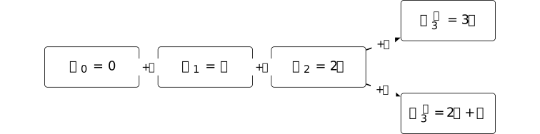
A deterministic history-only forecaster must return the same matrix \(\widehat W_3\) in both worlds. Since \(\|W_3^A-W_3^B\|_F=\|P-Q\|_F=\sqrt {2}\), the triangle inequality forces its Frobenius error to be at least \(1/\sqrt {2}\) on one continuation. Low-rank early motion therefore does not identify the next subspace or the next checkpoint.
Remark 4.4.13. Compression of a charted path is not capability acquisition [ftip-008B]AGENTDRAFTED
Remark 4.4.13. Compression of a charted path is not capability acquisition [ftip-008B]AGENTDRAFTED
NExt extracts global, local, and target differences from LoRA checkpoint matrices, keeps leading singular factors, learns a nonlinear predictor, jumps in that parameter chart, and resumes RLVR [chen2026lowrank, Sections 3.2, 4.1--4.3, and 5.1]. Its reported results are empirical; the paper states no theorem that a leading subspace remains stable or that a forecast preserves a policy.
The quantities in Definition 4.4.8--Definition 4.4.11 separate four tests. Squared singular-energy share concerns one matrix, spectral gap controls whether its leading subspace is identifiable, projector drift compares those subspaces over time, and path-emulation regret returns to fixed independent evaluation. None, by itself, is evidence that new feedback was acquired or that a new capability was learned. Such a claim must use a declared post-training gain such as Definition 1.3 and must charge forecast training, the parameter jump, and recovery updates.
5. Alignment gain and preference information [ftip-008E]AGENTDRAFTED
5. Alignment gain and preference information [ftip-008E]AGENTDRAFTED
Two finite models ask different questions about post-training. The first assumes an exact KL-regularized optimizer and characterizes the reward gain that its exponential tilt can produce. The second asks what ordinal comparisons reveal when post-training may reroute a fixed set of response circuits.
Neither source model is a general account of neural post-training. The first assumes exact optimization of a declared scalar reward. The second is a stylized routing model with a fixed circuit set. Extending the KL identity to an approximate optimizer requires further analysis. Extending the ordinal routing conclusion to a changing circuit set requires additional assumptions on that change.
5.1. Finite KL-regularized alignment [ftip-008F]AGENTDRAFTED
5.1. Finite KL-regularized alignment [ftip-008F]AGENTDRAFTED
This subsection studies an exact, finite optimization model. A reference law is exponentially tilted by a declared scalar reward. In this setting, reward gain admits two exact descriptions: a Jeffreys-divergence identity and a covariance under the reference law.
The statements do not model approximate optimization, neural training cost, reward validity, or independent capability evaluation.
Remark 5.1.1. Exact optimization on a finite response set [ftip-008G]AGENTDRAFTED
Remark 5.1.1. Exact optimization on a finite response set [ftip-008G]AGENTDRAFTED
Theorems 1 and 2 of the v1 preprint [paes2026theoretical] concern an exactly optimal KL-regularized policy and a fixed query. On a finite response set, their expectations and normalizers are ordinary finite sums.
These exact identities do not establish a comparison among best-of-\(N\), PPO, and GRPO, or a general guarantee for proxy rewards and reward ensembles. Those questions require assumptions beyond exact optimization of one reward.
Notation 5.1.2. Translating the alignment source notation [ftip-008H]AGENTDRAFTED
Notation 5.1.2. Translating the alignment source notation [ftip-008H]AGENTDRAFTED
The source writes \(\lambda >0\) for the KL penalty. Here we write \(\beta >0\), matching the DPO notation in Notation [ftip-003M]--Definition [ftip-003O]. This avoids collision with the generalized-advantage parameter in Definition [ftip-003E] and the protocol law in Definition 4.3.1.
The source's gain \(\Delta (r,r')\) is written \(G_p(r;s)\): \(r\) is the reward used to tilt the reference law \(p\), while \(s\) is the reward used to evaluate the tilted law. This avoids collision with both the simplex notation \(\Delta (X)\) of Notation [ftip-000A] and the paired DPO margin of Notation [ftip-003M]. For a finite set \(\mathcal Y\), a law \(p\in \Delta (\mathcal Y)\), and functions \(f,g:\mathcal Y\to \mathbb R\), set
\[ \operatorname {Cov}_p(f,g) =\mathbb E_{y\sim p}[f(y)g(y)] -\mathbb E_{y\sim p}[f(y)]\, \mathbb E_{y\sim p}[g(y)]. \]
Definition 5.1.3. Finite KL-alignment instance [ftip-008I]AGENTDRAFTED
Definition 5.1.3. Finite KL-alignment instance [ftip-008I]AGENTDRAFTED
A finite KL-alignment instance consists of a nonempty finite response set \(\mathcal Y\), a reference law \(p\in \Delta (\mathcal Y)\), a penalty \(\beta >0\), and finite real functions \(r,s:\mathcal Y\to \mathbb R\). The reference support is
\[ S_p=\{y\in \mathcal Y:p(y)>0\}. \]A prompt is fixed and suppressed. The function \(r\) determines the alignment update; \(s\) measures its result. They may coincide, but they need not. Finiteness makes every exponential weight and expectation below finite.
These objects specialize the fixed-query setting in [paes2026theoretical, Section 2, equations (2.1)--(2.2)]; they are not a definition of alignment in general.
Definition 5.1.4. Exponential weight and partition function [ftip-008J]AGENTDRAFTED
Definition 5.1.4. Exponential weight and partition function [ftip-008J]AGENTDRAFTED
For a finite KL-alignment instance, define the exponential weight and partition function by
\[ a_r(y)=\exp \left (\frac {r(y)}{\beta }\right ), \qquad Z_r=\mathbb E_{y\sim p}[a_r(y)]. \]Every \(a_r(y)\) is finite and strictly positive. Since \(p\) is a probability law on a nonempty finite set, \(0<Z_r<\infty \).
This weight and normalizer are the fixed-query form of [paes2026theoretical, Equation (2.2)].
Definition 5.1.5. Aligned law in finite-source notation [ftip-008K]AGENTDRAFTED
Definition 5.1.5. Aligned law in finite-source notation [ftip-008K]AGENTDRAFTED
The aligned law induced by \(r\) is \(q_r\in \Delta (\mathcal Y)\) given by
\[ q_r(y)=\frac {p(y)a_r(y)}{Z_r}. \]Normalization follows from the definition of \(Z_r\). Moreover, \(q_r(y)>0\) exactly when \(p(y)>0\). This is the finite notation for the same exponential-tilt optimizer stated in Definition [ftip-003O]; support preservation was proved in Theorem 4.1.6.
This formula is [paes2026theoretical, Equation (2.2)]. It assumes the exact optimizer, not an iterate returned by a particular training algorithm.
Definition 5.1.6. Cross-reward gain under an alignment reward [ftip-008L]AGENTDRAFTED
Definition 5.1.6. Cross-reward gain under an alignment reward [ftip-008L]AGENTDRAFTED
The cross-reward gain from aligning with \(r\) and evaluating with \(s\) is
\[ G_p(r;s) =\mathbb E_{y\sim q_r}[s(y)] -\mathbb E_{y\sim p}[s(y)]. \]The semicolon records two roles. Its left argument changes the response law; its right argument scores both laws. Thus \(G_p(r;s)\) is not an independent evaluation unless \(s\) has separately been declared to serve that role.
This is the finite notation for \(\Delta (r,r')\) in Theorem 2, equation (3.4), of Theoretical limits of language model alignment[paes2026theoretical].
Definition 5.1.7. Jeffreys divergence [ftip-008M]AGENTDRAFTED
Definition 5.1.7. Jeffreys divergence [ftip-008M]AGENTDRAFTED
For probability laws \(p\) and \(q\) for which both terms are finite, their Jeffreys divergence is
\[ J(p,q) =D_{\mathrm {KL}}(p\Vert q) +D_{\mathrm {KL}}(q\Vert p). \]The KL divergence and its argument order are defined in Definition [ftip-006X]. Unlike either directed term, \(J(p,q)=J(q,p)\). In the finite tilt of Definition 5.1.5, \(p\) and \(q_r\) have the same support, so both terms are finite.
Lemma 5.1.8. Log-density ratio of the exact tilt [ftip-008N]AGENTDRAFTED
Lemma 5.1.8. Log-density ratio of the exact tilt [ftip-008N]AGENTDRAFTED
For every \(y\in S_p\), the aligned law satisfies
\[ \log \frac {q_r(y)}{p(y)} =\frac {r(y)}{\beta }-\log Z_r. \]
Proof.
Proof.
On \(S_p\), both \(p(y)\) and \(q_r(y)\) are positive. Dividing the formula of Definition 5.1.5 by \(p(y)\) and taking logarithms gives the identity.
This is equation (B.1) followed by the logarithmic step in [paes2026theoretical, Appendix B.1, equations (B.1)--(B.2)].
Theorem 5.1.9. Exact reward gain equals scaled Jeffreys divergence [ftip-008O]AGENTDRAFTED
Theorem 5.1.9. Exact reward gain equals scaled Jeffreys divergence [ftip-008O]AGENTDRAFTED
For a finite KL-alignment instance,
\[ G_p(r;r)=\beta J(p,q_r). \]
Proof.
Proof.
Rearranging Lemma 5.1.8 gives \(r(y)=\beta \log (q_r(y)/p(y))+\beta \log Z_r\) on the common support. Taking expectation first under \(q_r\) and then under \(p\) yields
\[ \begin {aligned} \mathbb E_{q_r}[r] &=\beta D_{\mathrm {KL}}(q_r\Vert p)+\beta \log Z_r,\\ \mathbb E_p[r] &=-\beta D_{\mathrm {KL}}(p\Vert q_r)+\beta \log Z_r. \end {aligned} \]Subtracting cancels the common normalizer and gives the result.
This is the finite form of [paes2026theoretical, Theorem 1, equation (3.2), with proof in Appendix B.1].
Remark 5.1.10. What the Jeffreys identity does and does not identify [ftip-008P]AGENTDRAFTED
Remark 5.1.10. What the Jeffreys identity does and does not identify [ftip-008P]AGENTDRAFTED
The identity Theorem 5.1.9 is an equality inside one declared model. It says that exact gain in the optimizing reward equals a symmetric divergence from the reference law. It does not say that a larger divergence improves a different utility, nor that a training algorithm reaches the exact tilt.
The identity accounts for neither rollout and update work nor the cost of obtaining \(r\). Consequently it is not, by itself, a bound on the costed post-training potential of Definition 1.10.
Theorem 5.1.11. Cross-reward gain is a base-law covariance [ftip-008Q]AGENTDRAFTED
Theorem 5.1.11. Cross-reward gain is a base-law covariance [ftip-008Q]AGENTDRAFTED
For a finite KL-alignment instance,
\[ G_p(r;s) =\operatorname {Cov}_p\left (s,\frac {a_r}{Z_r}\right ). \]
Proof.
Proof.
The aligned expectation can be written under the reference law as \(\mathbb E_{q_r}[s]=\mathbb E_p[s a_r/Z_r]\). Also \(\mathbb E_p[a_r/Z_r]=1\). Substituting these two identities into Definition 5.1.6 gives the covariance defined in Notation 5.1.2.
This is the finite form of Theorem 2, equation (3.4), in Theoretical limits of language model alignment[paes2026theoretical]. Its proof is in Appendix B.1, equations (B.5)--(B.7).
Remark 5.1.12. The covariance is predictive only for a declared reward [ftip-008R]AGENTDRAFTED
Remark 5.1.12. The covariance is predictive only for a declared reward [ftip-008R]AGENTDRAFTED
The identity Theorem 5.1.11 expresses exact tilted-law gain using expectations under \(p\). This makes the population quantity accessible from the reference law in principle. A finite-sample estimator still needs its own sampling law, moment assumptions, and error analysis.
The formula also remains indexed by both \(r\) and \(s\). It cannot turn a proxy reward into an independent utility. If \(s=r\), it measures improvement in the same quantity that defined the exact optimizer; if \(s\ne r\), its sign is determined by the displayed covariance.
Example 5.1.13. A two-response alignment identity [ftip-008S]AGENTDRAFTED
Example 5.1.13. A two-response alignment identity [ftip-008S]AGENTDRAFTED
Take \(\mathcal Y=\{a,b\}\), \(p=(1/2,1/2)\), \(\beta =1\), and \(r(a)=0\), \(r(b)=\log 3\). Exponential weighting changes the reference law as follows.

The reward gain is
\[ G_p(r;r) =\left (\frac 34-\frac 12\right )\log 3 =\frac 14\log 3. \]Direct calculation gives
\[ \begin {aligned} D_{\mathrm {KL}}(q_r\Vert p) &=\frac 14\log \frac 12+\frac 34\log \frac 32,\\ D_{\mathrm {KL}}(p\Vert q_r) &=\frac 12\log 2+\frac 12\log \frac 23, \end {aligned} \]whose sum is \(\frac 14\log 3\). Thus the example checks Theorem 5.1.9 exactly; it is not an empirical alignment result.
Corollary 5.1.14. Averaging the fixed-query identity over prompts [ftip-008T]AGENTDRAFTED
Corollary 5.1.14. Averaging the fixed-query identity over prompts [ftip-008T]AGENTDRAFTED
Let \(\mathcal X\) be finite with prompt law \(\mu \). For each \(x\in \mathcal X\), let \(p_x\), \(r_x\), and \(q_{r_x}\) be a finite KL-alignment instance with the same penalty \(\beta >0\). Then
\[ \sum _{x\in \mathcal X}\mu (x)G_{p_x}(r_x;r_x) =\beta \sum _{x\in \mathcal X}\mu (x)J(p_x,q_{r_x}). \]
Proof.
Proof.
Apply Theorem 5.1.9 at each prompt and take the finite \(\mu \)-weighted sum.
The source theorem is stated for each fixed query. This corollary performs only finite averaging; it does not introduce a shared neural parameterization across prompts.
Lemma 5.1.15. Additive reward shifts leave the aligned law unchanged [ftip-008U]AGENTDRAFTED
Lemma 5.1.15. Additive reward shifts leave the aligned law unchanged [ftip-008U]AGENTDRAFTED
For constants \(c,d\in \mathbb R\),
\[ q_{r+c}=q_r, \qquad G_p(r+c;s+d)=G_p(r;s). \]
Proof.
Proof.
The shifted weight is \(a_{r+c}=e^{c/\beta }a_r\), while its partition function is \(Z_{r+c}=e^{c/\beta }Z_r\); the common factor cancels in the aligned law. Adding \(d\) to the evaluation reward adds \(d\) to both expectations in the gain, so it also cancels.
This finite lemma records the same prompt-dependent additive non-identifiability that appears in the DPO reparameterization of Definition [ftip-003P].
Remark 5.1.16. A penalty coefficient is not a hard KL budget [ftip-008V]AGENTDRAFTED
Remark 5.1.16. A penalty coefficient is not a hard KL budget [ftip-008V]AGENTDRAFTED
For fixed \(\beta \), the exponential tilt solves the penalized problem
\[ \max _{q\in \Delta (\mathcal Y)} \left \{\mathbb E_q[r] -\beta D_{\mathrm {KL}}(q\Vert p)\right \} \]under the conventions of Definition 5.1.3. This is not the same specification as choosing a number \(\kappa \) and solving
\[ \max _q\mathbb E_q[r] \quad \text {subject to}\quad D_{\mathrm {KL}}(q\Vert p)\leq \kappa . \]A Lagrange multiplier can relate the two problems when the relevant duality and activity conditions hold. The coefficient \(\beta \) alone does not declare a hard budget, and the identities Theorem 5.1.9--Theorem 5.1.11 do not supply those conditions.
Remark 5.1.17. Fixed-query identities and their assumptions [ftip-008W]AGENTDRAFTED
Remark 5.1.17. Fixed-query identities and their assumptions [ftip-008W]AGENTDRAFTED
The source setup writes rewards as \(r(\mathbf x,\mathbf y)\), while the display of Theorem 1 reverses the two arguments in places. This subsection uses the setup order and then suppresses the fixed prompt. The source also moves between a dataset-level penalized objective and fixed-query identities. The finite-averaging result Corollary 5.1.14 makes that step explicit.
The identities specialize Theoretical limits of language model alignment[paes2026theoretical] to a finite response set. They require no extension to the full sequence space.
Finally, exact exponential tilting is a distributional optimizer. It does not account for rollout, gradient, optimizer, or systems cost, and it does not show that PPO, GRPO, DPO, or any frontier training run attains the displayed law. Applying the identities to a training run therefore requires a separate argument that its output law is the exact optimizer.
5.2. Preference-feedback distortion [ftip-008X]AGENTDRAFTED
5.2. Preference-feedback distortion [ftip-008X]AGENTDRAFTED
A finite routing model supports preference-distortion lower bounds in Sections 2--3 and Appendix A of The limits of preference data for post-training[zhao2025limits]. Cardinal queries permit a different guarantee under the hypotheses of Peeking behind the ordinal curtain: Improving distortion via cardinal queries[amanatidis2021peeking].
Both comparisons depend on the queries, circuits, routing maps, utility, feedback profile, algorithm, and comparator class. The noiseless and Bradley--Terry bounds retain those model restrictions.
Remark 5.2.1. The routing-model assumption behind preference limits [ftip-008Y]AGENTDRAFTED
Remark 5.2.1. The routing-model assumption behind preference limits [ftip-008Y]AGENTDRAFTED
The routing model and preference limits below are based on the v1 preprint The limits of preference data for post-training[zhao2025limits]. It models a pretrained system as a finite collection of response circuits plus learned maps that route queries to those circuits. Post-training changes the routing maps while retaining the circuit collection.
The noiseless lower bound is proved here under explicit pointwise response separation and a deterministic preference-only learner, whose returned router may be stochastic. Its finite partition estimate and cardinal-utility construction give a restricted reconstruction of the source rate; the proof does not establish a randomized-learner extension.
The routing model is a source assumption, not an architectural theorem about language models. In particular, its lower bounds do not prove that real post-training creates no circuits, that a neural network decomposes into the displayed objects, or that every preference-learning algorithm obeys the same bound outside this model.
Notation 5.2.2. Notation for the finite preference model [ftip-008Z]AGENTDRAFTED
Notation 5.2.2. Notation for the finite preference model [ftip-008Z]AGENTDRAFTED
The finite preference model uses the following symbols, corresponding to the notation of The limits of preference data for post-training[zhao2025limits]:
\[ \mathcal Q\mapsto Q,\qquad \mathcal R\mapsto Y,\qquad \mathcal S_0\mapsto C_0,\qquad \mathcal Z\mapsto H, \]\[ \Phi \mapsto \mathfrak E,\qquad \mathcal D\mapsto \mu _Q,\qquad M\mapsto \mathfrak m. \]Thus \(H\) denotes the source's finite internal-representation set, not a public interaction history. The family \(\mathfrak E\) contains admissible query encoders and is unrelated to the costed potential \(\Phi \) of Definition 1.10.
Definition 5.2.3. Queries, responses, and retained circuits [ftip-0090]AGENTDRAFTED
Definition 5.2.3. Queries, responses, and retained circuits [ftip-0090]AGENTDRAFTED
Following the formal model in Section 2 of The limits of preference data for post-training[zhao2025limits], let \(Q\) be a finite nonempty query set and \(Y\) a response set. A response circuit is a function \(c:Q\to Y\). The finite nonempty set \(C_0\) contains the circuits retained from the pretrained model.
The word ``circuit'' is source terminology for this abstract function. No claim is made here that an element of \(C_0\) is localized in a neural network or corresponds to one human-named capability.
Definition 5.2.4. Query representation and circuit routing [ftip-0091]AGENTDRAFTED
Definition 5.2.4. Query representation and circuit routing [ftip-0091]AGENTDRAFTED
Let \(H\) be a finite nonempty representation set and \(\mathfrak E\subseteq H^Q\) a finite nonempty family of admissible encoders. A query encoder is \(e\in \mathfrak E\). A circuit router is a map
\[ h:H\longrightarrow \Delta (C_0). \]For a query \(\xi \in Q\), the composition \(h(e(\xi ))\) is a law on the retained circuits. Sampling \(c\sim h(e(\xi ))\) and returning \(c(\xi )\) gives the response law. These are the two routing components in the source model [zhao2025limits, Section 2, ``Formal model''].
Definition 5.2.5. Pretrained and post-trained routing models [ftip-0092]AGENTDRAFTED
Definition 5.2.5. Pretrained and post-trained routing models [ftip-0092]AGENTDRAFTED
A routing model is a triple \(\mathfrak m=(e,h,C_0)\) with the types fixed in Definition 5.2.3--Definition 5.2.4. The pretrained model is \(\mathfrak m_0=(e_0,h_0,C_0)\). In the source intervention, a post-trained model may replace \(e_0\) and \(h_0\), but it retains exactly \(C_0\).
Write \(\mathfrak m(\xi )\) for the random response obtained by sampling \(c\sim h(e(\xi ))\) and returning \(c(\xi )\). The source sometimes writes this as though the router selected a circuit rather than a distribution; the stochastic reading follows its declared codomain \(\Delta (C_0)\).
Definition 5.2.6. Utility and the uniform query law [ftip-0093]AGENTDRAFTED
Definition 5.2.6. Utility and the uniform query law [ftip-0093]AGENTDRAFTED
The source fixes the uniform probability law \(\mu _Q\) on \(Q\) and a utility function
\[ u:Q\times Y\longrightarrow \mathbb R. \]For a routing model \(\mathfrak m\), its expected utility is
\[ U_u(\mathfrak m) =\mathbb E_{\xi \sim \mu _Q} \mathbb E\left [u\left (\xi ,\mathfrak m(\xi )\right )\mid \xi \right ]. \]This is the outcome objective in [zhao2025limits, Section 2, ``Outcome-based optimization with preference data'']. It is an assumed cardinal utility, not something ordinal comparisons directly reveal.
Definition 5.2.7. Complete noiseless ordinal preference profile [ftip-0094]AGENTDRAFTED
Definition 5.2.7. Complete noiseless ordinal preference profile [ftip-0094]AGENTDRAFTED
Assume that distinct retained circuits never tie at a query. For each \(\xi \in Q\), utility then induces a strict comparison by
\[ c_i\succ _{\xi ,u}c_j \quad \Longleftrightarrow \quad u\left (\xi ,c_i(\xi )\right ) >u\left (\xi ,c_j(\xi )\right ). \]The complete noiseless ordinal profile is \(\succ _u=(\succ _{\xi ,u})_{\xi \in Q}\). The source gives the learner unlimited, unbiased access to every such comparison [zhao2025limits, Section 2, final paragraph]. Utilities with ties require a separately declared deterministic tie-break; the lower bounds below use the source's tie-free constructions.
Remark 5.2.8. Full preference data and an online oracle expose the same source information [ftip-0095]AGENTDRAFTED
Remark 5.2.8. Full preference data and an online oracle expose the same source information [ftip-0095]AGENTDRAFTED
Within this finite model, a table containing every comparison in \(\succ _u\) and a noiseless online oracle that answers every possible query expose the same ordinal information. The source deliberately grants this ideal access so that its obstruction is not caused by finite sampling or an offline split [zhao2025limits, Section 2].
This equivalence does not price the number of queries, labeler time, or adaptivity. It therefore cannot be transferred to a finite-feedback protocol without a separate query-complexity statement.
Definition 5.2.9. Preference-only post-training algorithm and attainable route class [ftip-0096]AGENTDRAFTED
Definition 5.2.9. Preference-only post-training algorithm and attainable route class [ftip-0096]AGENTDRAFTED
A preference-only post-training algorithm \(\mathcal A\) maps the pretrained routing model and the complete profile to
\[ \mathfrak m_{\mathcal A}(u) =\mathcal A(\mathfrak m_0,\succ _u). \]The deterministic comparator class displayed in the source theorems is
\[ \mathcal M_{\rm det}(C_0) =\left \{(e,h,C_0):e\in \mathfrak E, h:H\to C_0\right \}. \]The source's formal model initially permits stochastic routers \(h:H\to \Delta (C_0)\), but its theorem comparator uses deterministic \(h:H\to C_0\). The comparator class is therefore the displayed deterministic class.
Definition 5.2.10. Multiplicative post-training distortion [ftip-0097]AGENTDRAFTED
Definition 5.2.10. Multiplicative post-training distortion [ftip-0097]AGENTDRAFTED
Let \(\mathcal B\) be any post-training algorithm with output \(\mathfrak m_{\mathcal B}(u)\) under the feedback law induced by \(u\). When the denominator is positive, define its multiplicative post-training distortion by
\[ \operatorname {Dist}_u(\mathcal B;\mathfrak m_0) =\frac { \max _{\mathfrak m^*\in \mathcal M_{\rm det}(C_0)}U_u(\mathfrak m^*) }{ U_u(\mathfrak m_{\mathcal B}(u)) }. \]If the numerator is positive and the denominator is zero, set the ratio to \(+\infty \). The source lower bounds construct bounded nonnegative utilities for which the comparison is well defined [zhao2025limits, Equation (2) and Appendix A]. Distortion measures loss relative to the declared comparator class; it is not an absolute capability score.
Definition 5.2.11. Borda count [ftip-0098]AGENTDRAFTED
Definition 5.2.11. Borda count [ftip-0098]AGENTDRAFTED
Let \(m=|C_0|\), and suppose each \(\succ _{\xi ,u}\) is a strict total order on \(C_0\). If \(\operatorname {rank}_{\succ _{\xi ,u}}(c)\) places the most preferred circuit at rank one, its Borda score is
\[ B_{\xi }(c)=m-\operatorname {rank}_{\succ _{\xi ,u}}(c). \]The Borda-count choice is any circuit in
\[ \operatorname *{arg\,max}_{c\in C_0} \sum _{\xi \in Q}B_{\xi }(c). \]This is [zhao2025limits, Definition 3.1]. The source cites a prior equivalence between a standard RLHF model and Borda count; the definition here does not assert that every RLHF implementation is a Borda rule.
Example 5.2.12. A compromise circuit can maximize utility without winning Borda count [ftip-0099]AGENTDRAFTED
Example 5.2.12. A compromise circuit can maximize utility without winning Borda count [ftip-0099]AGENTDRAFTED
Example 3.2 of The limits of preference data for post-training[zhao2025limits] prints only \(a\geq 0\) and \(2a<b\), but those conditions do not force its stated rankings or Borda totals. Sufficient conditions are \(0<a<1/2\) and \(2a<b<1\). Take three queries, three circuits, and a singleton representation set, so every query must use one common circuit. Set
\[ \begin {array}{c|ccc} &c_A&c_B&c_C\\ \hline \xi _1&1&0&1-a\\ \xi _2&1&0&1-a\\ \xi _3&0&1&b \end {array} \]These inequalities give the rankings \(c_A\succ c_C\succ c_B\) for \(\xi _1,\xi _2\) and \(c_B\succ c_C\succ c_A\) for \(\xi _3\). Hence the Borda totals are \((4,2,3)\), so the ordinal rule selects \(c_A\). The utility totals are \((2,1,2-2a+b)\). Since \(2a<b\), circuit \(c_C\) has strictly greater total utility than \(c_A\).
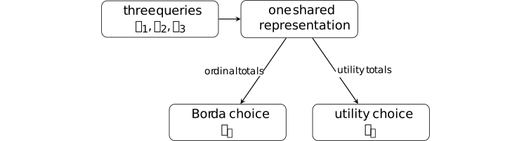
This finite example isolates information lost by ranking. The compromise circuit is never first for an individual query, yet its aggregate utility is largest. It does not show that Borda is always suboptimal or that a neural model must collapse all queries to one representation.
Theorem 5.2.13. Noiseless preference distortion for deterministic learners [ftip-009A]AGENTDRAFTED
Theorem 5.2.13. Noiseless preference distortion for deterministic learners [ftip-009A]AGENTDRAFTED
Let \(Q,H\) be nonempty finite sets, let \(\varnothing \neq \mathfrak E\subseteq H^Q\) be finite, and let \(C_0=\{c_1,\ldots ,c_m\}\) be a nonempty finite set of deterministic maps \(Q\to Y\). Write \(N=|Q|\), \(r=|H|\), \(p=|\mathfrak E|\) and \(m=|C_0|\). The query law is uniform on \(Q\). Call \(C_0\) pointwise response-separating when
\[ c_i\neq c_j\quad \Longrightarrow \quad c_i(q)\neq c_j(q) \qquad (q\in Q). \]Assume this separation. Let \(\mathcal A\) be a deterministic preference-only learner: from a pretrained model \(\mathfrak m_0\) and the complete strict ordinal profile, it returns \((e,h,C_0)\) with \(e\in \mathfrak E\) and a possibly stochastic router \(h:H\to \Delta (C_0)\). The comparator class is exactly \(\mathcal M_{\rm det}(C_0)\) of Definition 5.2.9, including every map \(H\to C_0\) for each \(e\in \mathfrak E\).
For every such pretrained model and learner there exists \(u:Q\times Y\to [0,1]\), inducing a strict profile, such that
\[ \sum _{j=1}^m u(q,c_j(q))=1\quad (q\in Q), \]\[ R_{Q,\mathfrak E,H}=\frac {N}{\sqrt {N(r+\log p)}+r}, \]\[ \operatorname {Dist}_u(\mathcal A;\mathfrak m_0) \geq \frac 1{80}\min \{\sqrt m,R_{Q,\mathfrak E,H}\}. \]Logarithms are natural. Utility averages over the uniform query and the learner's router draw as in Definition 5.2.6. The comparator maximum exists because its class is finite and nonempty. It is positive for the normalized utilities above: some constant-circuit route has mean at least \(1/m\). A zero learner utility therefore gives distortion \(+\infty \), with no \(0/0\) case.
Proof.
Proof.
First, for every normalized nonnegative utility, the comparator value is at least the learner value. Keep the learner's representation map and, on each fiber, choose a circuit maximizing its total utility there. That deterministic choice dominates the stochastic mixture and belongs to the comparator class. Thus distortion is at least one.
Put
\[ \begin {aligned} D&=\sqrt {Nr}+\sqrt {\frac N2\log (4p)},& B&=\sqrt {N(r+\log p)},\\ T&=\min \{\sqrt m,R_{Q,\mathfrak E,H}\},& x&=\min \{\sqrt m,N/(2D)\}. \end {aligned} \]Since \((\log 4)/2<1\leq r\) and \(\log p\geq 0\), we have \(D\leq 2B\). Consequently \(N/(2D)\geq N/(4B)\geq R_{Q,\mathfrak E,H}/4\) and \(x\geq T/4\). Every denominator is positive.
If \(m=1\), assign utility one to the sole circuit response at every query. Distortion is one and \(T\leq 1\). If \(m\geq 2\) but \(x<2\), assign the same strict normalized values \(2(m-j)/(m(m-1))\) to the circuits in index order at every query. Distortion is at least one and \(T<8\), which proves the claimed bound. Extend both assignments by zero to all other responses.
In the remaining case set \(k=\lfloor x\rfloor \). Then
\[ 2\leq k\leq \sqrt m,\qquad kD\leq N/2, \qquad k\geq x/2\geq T/8. \]Write \([k]=\{1,\ldots ,k\}\) and fix a map \(f:Q\to [k]\) supplied by Lemma 5.2.15. At a query with label \(i=f(q)\), fix the strict order putting \(c_i\) first and the remaining circuits in increasing index order. Let \(\operatorname {rank}_i(j)\in \{1,\ldots ,m\}\) be the position of \(c_j\), with the first circuit at rank one, and define
\[v_i(j)=\frac {2(m-\operatorname {rank}_i(j))}{m(m-1)}.\]These values decrease strictly in the fixed order, sum to one and lie in \([0,2/m]\). The ordinal profile is now fixed independently of the learner's output. Run the deterministic learner on this profile and \(\mathfrak m_0\), obtaining \((e,h,C_0)\). Write \(h_z(j)=h(z)(c_j)\) for the probability of circuit \(c_j\) at representation \(z\). For each \(z\in H\), choose \(i_z\in [k]\) minimizing \(h_z(j)\) over \(j\in [k]\), breaking ties by index. Since \(\sum _{j=1}^k h_z(j)\leq 1\), we have \(h_z(i_z)\leq1/k\).
Let \(A=\{q:f(q)=i_{e(q)}\}\) and \(S=|A|\). The lower partition bound gives
\[ S=\sum _zX_{z,i_z}\geq \sum _z\min _{j\in [k]}X_{z,j} \geq N/k-D\geq N/(2k). \]Fix \(\epsilon =1/4\). For \(i=f(q)\), assign
\[ u(q,c_j(q))= \begin {cases} (1-\epsilon )\mathbf 1_{j=i}+\epsilon v_i(j),&q\in A,\\ (1-\epsilon )/m+\epsilon v_i(j),&q\notin A. \end {cases} \]Each row is nonnegative and sums to one. On selected queries the added peak favors the already highest-ranked circuit; on the other queries the same constant is added to every circuit. Hence every row induces exactly the fixed strict order. Pointwise response separation makes these assignments well-defined on \(Q\times Y\); assign zero to responses outside the attained circuit responses. Because the final utility has the unchanged ordinal profile, the deterministic learner returns the same \((e,h,C_0)\).
Write \(W=NU\) for total utility. A selected query gives the learner at most \((1-\epsilon )/k+2\epsilon/m\); any other query gives at most \((1-\epsilon )/m+2\epsilon/m\). Averaging over the stochastic router yields
\[ W_{\mathcal A} \leq (1-\epsilon )S/k+(1-\epsilon )(N-S)/m+2\epsilon N/m \leq S/k+2N/m. \]Choose the deterministic comparator \(e^*=e\) and \(h^*(z)=c_{i_z}\). It belongs to the declared class, attains utility at least \(1-\epsilon \geq1/2\) on each selected query and nonnegative utility elsewhere. Thus its total utility is at least \(S/2\). If learner utility is zero the bound follows. Otherwise, using \(S\geq N/(2k)\) and \(k^2\leq m\),
\[ \begin {aligned} \operatorname {Dist}_u &\geq \frac {S/2}{S/k+2N/m} =\frac {k}{2(1+2kN/(mS))}\\ &\geq \frac {k}{2(1+4k^2/m)} \geq \frac {k}{10}\geq \frac {T}{80}. \end {aligned} \]Appendix Theorem A.1 of The limits of preference data for post-training[zhao2025limits] states the corresponding rate for its routing model. Its displayed balancing parameter retains \(\log N\) factors that are absent from its final rate; the second-moment partition bound in Lemma 5.2.15 supplies a separate argument for the stated restricted model. Its index-based perturbation on queries outside the selected group need not preserve their prescribed favorite; the query-dependent rank weights used here preserve it. When circuits collide at a query, a circuitwise prescription need not define a response utility; pointwise separation excludes that issue.
The utility is a worst-case existential choice for each fixed learner. The proof permits stochastic inference, but it does not cover internal learner randomness: a utility chosen after a realized random output need not be one utility valid before the learner's random draw. No claim about response-colliding circuits or the separate noisy-preference bound follows.
Corollary 5.2.14. A square-root corollary under explicit query growth [ftip-009B]AGENTDRAFTED
Corollary 5.2.14. A square-root corollary under explicit query growth [ftip-009B]AGENTDRAFTED
Under all hypotheses of Theorem 5.2.13, including a deterministic preference-only learner and pointwise response separation, assume
\[R_{Q,\mathfrak E,H}\geq \sqrt {|C_0|}.\]For every pretrained model and every such learner, the utility supplied by that theorem satisfies
\[ \operatorname {Dist}_u(\mathcal A;\mathfrak m_0) \geq \frac 1{80}\sqrt {|C_0|}. \]
Proof.
Proof.
The displayed growth condition makes the minimum in Theorem 5.2.13 equal to \(\sqrt {|C_0|}\).
Theorem 3.3 of The limits of preference data for post-training[zhao2025limits] gives a square-root rate in its large-query regime. The explicit condition above gives a finite regime for the reconstructed theorem with its stated learner and response assumptions.
Lemma 5.2.15. A simultaneous finite partition bound [ftip-009C]AGENTDRAFTED
Lemma 5.2.15. A simultaneous finite partition bound [ftip-009C]AGENTDRAFTED
Let \(Q,H\) be nonempty finite sets with \(N=|Q|\) and \(r=|H|\), and let \(\mathfrak E\subseteq H^Q\) be nonempty and finite with \(p=|\mathfrak E|\). For every integer \(k\geq 1\), there is a map \(f:Q\to [k]\) such that, simultaneously for every \(e\in \mathfrak E\),
\[ \begin {aligned} \sum _{z\in H}\max _{j\in [k]}X_{z,j}&\leq \frac Nk+D,\\ \sum _{z\in H}\min _{j\in [k]}X_{z,j}&\geq \frac Nk-D, \end {aligned} \]where \([k]=\{1,\ldots ,k\}\), logarithms are natural, and
\[ X_{z,j}=|\{q\in Q:e(q)=z,\ f(q)=j\}|, \qquad D=\sqrt {Nr}+\sqrt {\frac N2\log (4p)}. \]
Proof.
Proof.
Choose the labels \(f(q)\) independently and uniformly from \([k]\). Fix \(e,z\), write \(n_z=|e^{-1}(z)|\), and put \(a_j=X_{z,j}-n_z/k\). Each occupancy has variance \(n_z(1/k)(1-1/k)\), so
\[\mathbb E\sum _{j=1}^k a_j^2=n_z(1-1/k).\]The pointwise maximum and minimum satisfy
\[ \begin {aligned} \max _jX_{z,j}&\leq n_z/k+\|a\|_2,\\ \min _jX_{z,j}&\geq n_z/k-\|a\|_2. \end {aligned} \]Jensen's inequality gives \(\mathbb E\|a\|_2\leq \sqrt {n_z(1-1/k)}\). Summing over \(z\) and applying Cauchy--Schwarz yields
\[ \begin {aligned} \mathbb E\sum _z\max _jX_{z,j}&\leq N/k+\sqrt {Nr(1-1/k)},\\ \mathbb E\sum _z\min _jX_{z,j}&\geq N/k-\sqrt {Nr(1-1/k)}. \end {aligned} \]Changing one label changes only one representation group: one occupancy decreases by one and another increases by one. Its maximum and its minimum each change by at most one. Thus both sums have bounded differences with all \(N\) constants equal to one. McDiarmid's inequality, also used in Appendix A.1 of The limits of preference data for post-training[zhao2025limits], bounds each relevant one-sided deviation of size \(t\) by \(\exp (-2t^2/N)\).
Choose \(t=\sqrt {(N/2)\log (4p)}\). A union bound over both tails and all \(p\) representations gives total failure probability at most
\[2p\exp (-2t^2/N)=\frac 12<1.\]At least one deterministic labeling satisfies both claimed bounds, since \(\sqrt {Nr(1-1/k)}\leq \sqrt {Nr}\). Empty representation fibers have all occupancies zero and require no exception.
The bound uses a second-moment estimate in place of the occupancy estimate in source Lemma A.2. The chosen labeling depends only on \(Q,H,\mathfrak E,k\); its existence uses proof randomness and does not assume randomness in the learning algorithm.
Definition 5.2.16. Bradley--Terry preference from a score map [ftip-009D]AGENTDRAFTED
Definition 5.2.16. Bradley--Terry preference from a score map [ftip-009D]AGENTDRAFTED
Fix a query \(\xi \) and nonnegative circuit scores \(a_{\xi ,c}\geq 0\) such that \(a_{\xi ,c_i}+a_{\xi ,c_j}>0\) for every compared pair. The Bradley--Terry comparison law is
\[ \Pr (c_i\succ _{\xi }c_j) =\frac {a_{\xi ,c_i}} {a_{\xi ,c_i}+a_{\xi ,c_j}}. \]Only score ratios are identified: multiplying every score for a fixed query by the same positive constant leaves all comparison probabilities unchanged. The linear and exponential score links discussed in [zhao2025limits, Section 3.2] therefore impose different assumptions on the relation between rewards and comparisons.
Definition 5.2.17. Exponential-score Bradley--Terry feedback [ftip-009E]AGENTDRAFTED
Definition 5.2.17. Exponential-score Bradley--Terry feedback [ftip-009E]AGENTDRAFTED
The exponential-score link sets
\[ a_{\xi ,c}=\exp \left (u(\xi ,c(\xi ))\right ). \]For this link, exact comparison probabilities reveal pairwise utility differences through
\[ \log \frac {\Pr (c_i\succ _{\xi }c_j)} {\Pr (c_j\succ _{\xi }c_i)} =u(\xi ,c_i(\xi ))-u(\xi ,c_j(\xi )). \]This algebra explains why a known link and infinite noiseless frequency information can expose more than an ordinal order. It does not apply when the link is unknown or misspecified.
Definition 5.2.18. Linear-score Bradley--Terry feedback [ftip-009F]AGENTDRAFTED
Definition 5.2.18. Linear-score Bradley--Terry feedback [ftip-009F]AGENTDRAFTED
The linear-score link sets
\[ a_{\xi ,c}=u(\xi ,c(\xi )), \qquad \Pr (c_i\succ _{\xi }c_j) =\frac {u(\xi ,c_i(\xi ))} {u(\xi ,c_i(\xi ))+u(\xi ,c_j(\xi ))}. \]Write \(p^u_{\xi ,ij}\) for the displayed probability and define the complete pairwise-probability profile
\[ P_u^{\rm lin} =\left (p^u_{\xi ,ij}\right )_{\xi \in Q,\,c_i\neq c_j\in C_0}. \]This requires nonnegative utilities and a positive denominator for each queried pair. A linear-score algorithm \(\mathcal A_{\rm lin}\) takes \((\mathfrak m_0,P_u^{\rm lin})\) as input and returns \(\mathfrak m_{\mathcal A_{\rm lin}}(u)\). The following lower bound concerns this specific link; it is not a lower bound for every stochastic preference model.
Theorem 5.2.19. General linear-score noisy preference lower bound [ftip-009G]AGENTDRAFTED
Theorem 5.2.19. General linear-score noisy preference lower bound [ftip-009G]AGENTDRAFTED
Assume pointwise response separation as defined in Theorem 5.2.13. For every pretrained routing model and linear-score algorithm \(\mathcal A_{\rm lin}\), there exists a utility
\[ u:Q\times Y\longrightarrow [0,1]. \]Post-training from even the complete comparison-probability profile of the linear-score link then satisfies
\[ \operatorname {Dist}_u(\mathcal A_{\rm lin};\mathfrak m_0) \geq \widetilde \Omega \left ( \min \left \{|C_0|,R_{Q,\mathfrak E,H}\right \} \right ), \]where \(R_{Q,\mathfrak E,H}\) is defined in Theorem 5.2.13. The theorem is again existential in \(u\) and uses the source's deterministic comparator. The same circuitwise-utility issue recorded in Theorem 5.2.13 prevents us from asserting the source's unrestricted pretrained-model quantifier here. Its noise is informative because probabilities depend on cardinal scores; the obstruction survives under the particular linear link.
This lower bound is the form of Appendix Theorem A.5 in The limits of preference data for post-training[zhao2025limits] with the additional pointwise response-separation assumption stated above.
Remark 5.2.20. The noisy main theorem and appendix have different asymptotic notation [ftip-009H]AGENTDRAFTED
Remark 5.2.20. The noisy main theorem and appendix have different asymptotic notation [ftip-009H]AGENTDRAFTED
The main-text Theorem 3.4 of The limits of preference data for post-training[zhao2025limits] displays \(\Omega (|C_0|)\) in its stated large-query regime. Appendix Theorem A.5 displays the general bound with \(\widetilde \Omega \) and the minimum in Theorem 5.2.19. The tilde can hide logarithmic factors, so these statements are not textually identical.
The general bound in Theorem 5.2.19 has the appendix's rate with a possible logarithmic loss. Eliminating that loss to obtain the main-text rate requires an additional argument.
Definition 5.2.21. Cardinal value query [ftip-009I]AGENTDRAFTED
Definition 5.2.21. Cardinal value query [ftip-009I]AGENTDRAFTED
In the social-choice source, agents rank alternatives and also have nonnegative cardinal values. A value query takes an agent \(i\) and an alternative \(j\) and returns \(v_{ij}\) [amanatidis2021peeking, Definition 1].
Under the routing analogy, a query \(\xi \in Q\) plays the role of an agent and a circuit \(c\in C_0\) plays the role of an alternative. A cardinal query therefore reveals one value \(u(\xi ,c(\xi ))\). Query counts inherited from the social-choice theorem are per query/agent, not totals across \(Q\).
Theorem 5.2.22. Acceptable Range Voting information--distortion tradeoff [ftip-009J]AGENTDRAFTED
Theorem 5.2.22. Acceptable Range Voting information--distortion tradeoff [ftip-009J]AGENTDRAFTED
Let \(m\) be the number of alternatives and let \(k\in \{1,\ldots ,m\}\). Theorem 4 of Peeking behind the ordinal curtain: Improving distortion via cardinal queries[amanatidis2021peeking] states that \(k\)-Acceptable Range Voting uses
\[ O(k\log m) \]value queries per agent and has distortion
\[ O\left (m^{1/(k+1)}\right ). \]This is a social-choice mechanism theorem. It transfers directly to the singleton-representation specialization \(|H|=1\), where every query must use one common circuit. Under that restriction, queries are agents and circuits are alternatives as in Definition 5.2.21. The theorem does not by itself cover a routing comparator that may choose different circuits for different representations, and it is not an implementation of neural post-training.
This statement is Theorem 4 of Peeking behind the ordinal curtain: Improving distortion via cardinal queries[amanatidis2021peeking].
Corollary 5.2.23. Constant distortion with logarithmically many value queries per query [ftip-009K]AGENTDRAFTED
Corollary 5.2.23. Constant distortion with logarithmically many value queries per query [ftip-009K]AGENTDRAFTED
Taking \(k\) proportional to \(\log m\) in Theorem 5.2.22 yields constant distortion with
\[ O(\log ^2 m) \]value queries per agent. This is Corollary 2 of Peeking behind the ordinal curtain: Improving distortion via cardinal queries[amanatidis2021peeking], inherited as Theorem 3.5 by The limits of preference data for post-training[zhao2025limits]. Under the routing analogy, the count is per query, so a full table over \(|Q|\) queries can require \(O(|Q|\log ^2m)\) values. The statement is an upper bound for the named mechanism in the common-circuit specialization of Theorem 5.2.22. It is not a result for the full routing comparator, nor a lower bound saying that this many values are necessary.
Remark 5.2.24. Information and optimization assumptions in the two finite models [ftip-009L]AGENTDRAFTED
Remark 5.2.24. Information and optimization assumptions in the two finite models [ftip-009L]AGENTDRAFTED
The two source families assume different information models; the diagram compares them without imposing an information order.
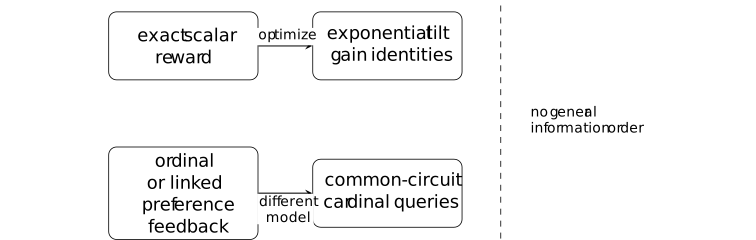
The KL identities characterize the exact optimizer for a declared scalar reward. The preference lower bounds are worst-case statements inside a fixed- circuit routing model. Bradley--Terry conclusions depend on the chosen score link. In the common-circuit specialization, cardinal queries change the information modality and admit a positive mechanism result. Outside that specialization, the preference and cardinal-query results are not directly comparable without further assumptions.
None of these statements derives the finite transcript theorem Theorem 4.3.5, and none proves that benchmark gain is capability acquisition. Applying either result to a training system requires that system to satisfy the corresponding information, optimizer, and comparator assumptions.
6. Controlled coverage, feedback resolution, and prompt breadth [ftip-009M]AGENTDRAFTED
6. Controlled coverage, feedback resolution, and prompt breadth [ftip-009M]AGENTDRAFTED
This section studies finite measurements and controlled comparisons that separate starting-policy coverage from the information supplied by a reward. It also records how a training prompt law limits the scope of an observed post-training effect.
The empirical route is a controlled language-model post-training study. Its reported outcomes remain experiment-specific observations. Theorems in this section follow from the stated finite-probability assumptions; the empirical results alone do not imply those conclusions.
6.1. Starting-policy interventions [ftip-009N]AGENTDRAFTED
6.1. Starting-policy interventions [ftip-009N]AGENTDRAFTED
A comparison among starting policies is meaningful only after the task, training grid, feedback rule, and evaluation procedure have been declared. Observed differences are conditional on those experimental coordinates.
Remark 6.1.1. The source experiment as an intervention matrix [ftip-009O]AGENTDRAFTED
Remark 6.1.1. The source experiment as an intervention matrix [ftip-009O]AGENTDRAFTED
[clay2026demystifying, Sections 4.1--4.3 and Figure 1] organize the reported experiments along three declared axes: a starting model distribution, a training-prompt distribution, and a reward function. Each reported measurement therefore belongs to a cell of a matrix rather than to an unqualified ``RL post-training'' condition. The source holds its broad training recipe fixed while varying selected axes; it does not study variation among RL algorithms.
Each experimental comparison is conditional on its model, task, prompt law, executable reward rule, training budget, and evaluation procedure. The reward rule is especially consequential here because the main text and Appendix C do not state identical sparse-reward semantics. Section 4.2 describes target containment with a length penalty. Appendix C's prose says an exact target receives unit reward, but its displayed equation requires the response to be strictly longer than the target for any positive reward. These two descriptions do not identify a single sparse-reward implementation.
Definition 6.1.2. Target-response event [ftip-009P]AGENTDRAFTED
Definition 6.1.2. Target-response event [ftip-009P]AGENTDRAFTED
Fix an evaluation instance \(x\), a response space \(\mathcal Y_x\), and a declared target predicate \(h_x^\star :\mathcal Y_x\to \{0,1\}\). For a sampled response \(Y\), the target-response event is
\[ E_x^\star =\{h_x^\star (Y)=1\}. \]The predicate is part of the evaluation specification. It may test exact string equality after a declared normalization, containment of a target substring, equality of a parsed answer, or another explicitly typed condition. These predicates are not interchangeable. The movie-quote and AIME experiments in [clay2026demystifying, Sections 4.1--4.2] use different response objects and therefore require different target predicates.
Remark 6.1.3. Exact-string success and task utility are different predicates [ftip-009Q]AGENTDRAFTED
Remark 6.1.3. Exact-string success and task utility are different predicates [ftip-009Q]AGENTDRAFTED
Let \(y_x^\star \) be a designated string and let \(N_x\) be a declared normalizer. Exact-string success is the specialization \(h_x^\star (y)=\mathbf 1\{N_x(y)=N_x(y_x^\star )\}\) of Definition 6.1.2. A task utility may instead accept semantically equivalent answers, assign partial credit, invoke a verifier, or depend on evaluator randomness as in Convention 1.1.
Consequently, a change in target-string match rate is not automatically a change in task utility. [clay2026demystifying, Sections 4.1--4.2] deliberately use narrow target behaviours to study controlled coverage. Transferring their measurements to broader capability requires a separately justified evaluator.
Definition 6.1.4. Base, SFT-positive, and SFT-negative starting-policy triple [ftip-009R]AGENTDRAFTED
Definition 6.1.4. Base, SFT-positive, and SFT-negative starting-policy triple [ftip-009R]AGENTDRAFTED
For one declared model family and target predicate, a starting-policy triple is
\[ \left (\pi ^{\mathrm {base}},\pi ^+,\pi ^-\right ). \]Here \(\pi ^{\mathrm {base}}\) is the unmodified starting policy, \(\pi ^+\) is obtained by a declared supervised update intended to increase target-response frequency, and \(\pi ^-\) is obtained by a declared update intended to decrease it. The superscripts name producing interventions, not mathematical order relations between the resulting policies.
[clay2026demystifying, Section 4.1] instantiates the triple with the source's Base, SFT-positive, and SFT-negative checkpoints. For the movie quote, its SFT mixture places twenty percent weight on the target quote and eighty percent on other quotes from the Cornell Movie-Dialogs corpus; the negative intervention maximizes cross-entropy loss on the target.
Remark 6.1.5. SFT-positive and SFT-negative are composite weight interventions [ftip-009S]AGENTDRAFTED
Remark 6.1.5. SFT-positive and SFT-negative are composite weight interventions [ftip-009S]AGENTDRAFTED
The policies \(\pi ^+\) and \(\pi ^-\) of Definition 6.1.4 are produced by optimization. Their weights, output probabilities, representations, and off-target behaviours can all change together. Calling one intervention ``positive'' and the other ``negative'' describes its intended effect on the declared target response; it does not assert that only one probability mass was edited.
The comparisons in [clay2026demystifying, Sections 4.1 and 5.1] therefore test dependence on three constructed starting checkpoints. They do not identify a causal effect of initial target probability alone without an additional intervention model.
Definition 6.1.6. Controlled post-training experiment cell [ftip-009T]AGENTDRAFTED
Definition 6.1.6. Controlled post-training experiment cell [ftip-009T]AGENTDRAFTED
A controlled post-training experiment cell is a record
\[ \mathfrak c= (M,\pi ^{\mathrm {init}},\mathsf T,\mathcal D_{\mathrm {tr}}, r^{\mathrm {id}},\mathcal A,b_{\mathrm {tr}},\mathsf E), \]where \(M\) identifies the model architecture and checkpoint lineage, \(\pi ^{\mathrm {init}}\) is its starting policy, \(\mathsf T\) is the task, \(\mathcal D_{\mathrm {tr}}\) is the training-prompt law, \(r^{\mathrm {id}}\) identifies an executable reward rule and version, \(\mathcal A\) is the update procedure, \(b_{\mathrm {tr}}\) is the training budget, and \(\mathsf E\) is the evaluation interface. Random seeds and hyperparameters belong to the relevant record fields even when suppressed from the notation.
[clay2026demystifying, Figure 1 and Sections 4.1--4.3] motivates the coordinates. The source varies starting distribution, prompt distribution, and reward while using a common broad RL setup. Because its main-text and Appendix-C sparse rewards differ, the reward field is an identifier for an executable rule, not merely the word ``sparse.''
Definition 6.1.7. Matched cells and held-fixed coordinates [ftip-009U]AGENTDRAFTED
Definition 6.1.7. Matched cells and held-fixed coordinates [ftip-009U]AGENTDRAFTED
Let \(J\) index the coordinates of an experiment cell \(\mathfrak c\) from Definition 6.1.6. For \(S\subseteq J\), two cells \(\mathfrak c\) and \(\mathfrak c'\) are matched outside \(S\) when
\[ \mathfrak c_j=\mathfrak c'_j\qquad \text {for every }j\in J\setminus S. \]The coordinates in \(J\setminus S\) are the held-fixed coordinates; those in \(S\) are the declared intervention coordinates. Equality means equality at the resolution recorded by the experiment, including evaluation sample size when that size affects the reported statistic.
A matched comparison licenses a contrast between the recorded cells. It does not show that a named coordinate is internally atomic. In particular, matching outside the starting-policy coordinate leaves the composite-checkpoint qualification of Remark 6.1.5 in force.
Example 6.1.8. Three starting laws under one declared training grid [ftip-009V]AGENTDRAFTED
Example 6.1.8. Three starting laws under one declared training grid [ftip-009V]AGENTDRAFTED
A source comparison may place the three starting policies of Definition 6.1.4 into cells matched outside the starting-policy coordinate. The shared boxes below mean equality of the declared grid fields, not that the three checkpoints differ in only one scalar probability.
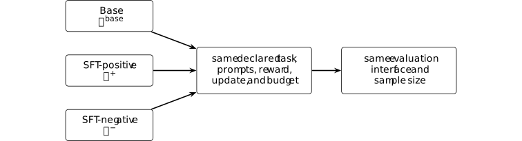
This is the comparison pattern used in [clay2026demystifying, Sections 4.1 and 5.1]. An actual cell still needs its model, task, reward implementation, and numerical record; the diagram is not a claim that all experiments in the paper instantiate one identical grid.
Remark 6.1.9. What the starting-policy comparison can and cannot identify [ftip-009W]AGENTDRAFTED
Remark 6.1.9. What the starting-policy comparison can and cannot identify [ftip-009W]AGENTDRAFTED
Within a declared model, task, training grid, and evaluation procedure, the three-cell comparison can establish that the measured post-training outcome differs across the source's constructed starting checkpoints. The movie-quote and AIME entries in [clay2026demystifying, Section 5.1, Tables 1--2] are empirical records of that form.
The comparison does not isolate initial target probability from every other SFT-induced weight change, prove that an observed zero has zero support, or establish acquisition of a broader capability. The reported model sets differ across the paper: [clay2026demystifying, Section 4.1] names OLMo 3, Qwen2-7B, Qwen3-1.7B, and Qwen2.5-7B-Instruct, while Table 1 and Appendix G also report Qwen3-8B and Qwen2-1.5B. Each measurement is specific to the model and configuration in its table row.
6.2. Finite initial-coverage measurement [ftip-009X]AGENTDRAFTED
6.2. Finite initial-coverage measurement [ftip-009X]AGENTDRAFTED
A finite evaluation records hits, not mathematical support. This subsection introduces the hit count and its sampling law, derives the exact zero-hit bound under independent sampling, and then returns to the limits of the source measurement.
Definition 6.2.1. Initial evaluation hit count [ftip-009Y]AGENTDRAFTED
Definition 6.2.1. Initial evaluation hit count [ftip-009Y]AGENTDRAFTED
Fix a starting policy, an evaluation sampling law, and the target predicate of Definition 6.1.2. Before post-training, draw evaluation records \((X_j,Y_j)_{j=1}^m\). Define the hit indicators and the initial evaluation hit count by
\[ I_j^\star =h_{X_j}^\star (Y_j), \qquad K_m=\sum _{j=1}^{m}I_j^\star . \]The sampling law determines whether the instances \(X_j\) are fixed, resampled, or stratified. The adjective ``initial'' locates the measurement before the post-training intervention; it does not assert that the samples are independent or that the starting policy is a foundation checkpoint.
Definition 6.2.2. Empirical initial success rate [ftip-009Z]AGENTDRAFTED
Definition 6.2.2. Empirical initial success rate [ftip-009Z]AGENTDRAFTED
For a nonempty initial evaluation sample of size \(m\), the empirical initial success rate is
\[ \widehat p_m=\frac {K_m}{m} =\widehat {\mathbb E}_{j\in \{1,\ldots ,m\}}[I_j^\star ], \]using the empirical-average convention of Convention [ftip-006Z]. This is a statistic of the declared sample. It is not, without a sampling model and an uncertainty statement, the exact successful-support probability \(p_P(x)\) of Definition 3.1.
Remark 6.2.3. Zero observed hits are not zero probability [ftip-00A0]AGENTDRAFTED
Remark 6.2.3. Zero observed hits are not zero probability [ftip-00A0]AGENTDRAFTED
The equality \(K_m=0\) says that no target response occurred in one finite sample. Every success probability \(0\leq p<1\) assigns positive probability \((1-p)^m\) to this observation under independent Bernoulli sampling. Thus \(\widehat p_m=0\) does not imply \(p=0\), absence from mathematical support, or impossibility of discovery under a larger budget.
The entries printed as 0.00 percent in [clay2026demystifying, Section 5.1, Tables 1--2] are empirical rates at the stated evaluation sizes. They must not be rewritten as exact support claims.
Theorem 6.2.4. Zero-hit likelihood under iid evaluation [ftip-00A1]AGENTDRAFTED
Theorem 6.2.4. Zero-hit likelihood under iid evaluation [ftip-00A1]AGENTDRAFTED
Let \(m\in \mathbb N_{\geq 1}\). Assume the hit indicators from Definition 6.2.1 are independent Bernoulli variables with a common success probability \(p\). Then \(K_m\) has the binomial law and
\[ \Pr _p(K_m=0)=(1-p)^m. \]
Proof.
Proof.
The event \(K_m=0\) is \(\bigcap _{j=1}^m\{I_j^\star =0\}\). Independence and \(\Pr _p(I_j^\star =0)=1-p\) give the displayed product.
This finite statement follows from the displayed hypotheses. Applying it to a source table requires the additional iid and stationary-success assumptions stated above.
Corollary 6.2.5. Exact one-sided bound after zero hits [ftip-00A2]AGENTDRAFTED
Corollary 6.2.5. Exact one-sided bound after zero hits [ftip-00A2]AGENTDRAFTED
Assume Theorem 6.2.4 with \(m\in \mathbb N_{\geq 1}\) and fix \(0<\delta <1\). If \(K_m=0\), inversion of the exact zero-count likelihood gives the one-sided upper endpoint
\[ u_{m,\delta }=1-\delta ^{1/m}. \]Indeed, \(\Pr _{u_{m,\delta }}(K_m=0)=\delta \), and for every \(p>u_{m,\delta }\) one has \(\Pr _p(K_m=0)<\delta \). Thus the observed zero count excludes probabilities above \(u_{m,\delta }\) at exact level \(\delta \) under the declared iid model.
Proof.
Proof.
By Theorem 6.2.4, the zero-count likelihood is \((1-p)^m\), which is strictly decreasing in \(p\). Solving \((1-p)^m=\delta \) gives the endpoint and the stated strict inequality.
This is a likelihood inversion derived from the displayed finite setup, not a source theorem and not a support certificate.
Example 6.2.6. The 128-sample zero-hit bound [ftip-00A3]AGENTDRAFTED
Example 6.2.6. The 128-sample zero-hit bound [ftip-00A3]AGENTDRAFTED
Take \(m=128\) and \(\delta =0.05\) in Corollary 6.2.5. After zero hits, the exact one-sided upper endpoint is
\[ u_{128,0.05} =1-0.05^{1/128} \approx 0.02313. \]Under the iid Bernoulli model, probabilities above approximately 2.313 percent make a zero count less than five percent likely. The calculation does not turn a recorded \(0/128\) into proof that the true probability is zero, and it does not apply if the 128 evaluations have a different joint sampling law.
Definition 6.2.7. First positive sparse-reward time [ftip-00A4]AGENTDRAFTED
Definition 6.2.7. First positive sparse-reward time [ftip-00A4]AGENTDRAFTED
Fix an executable sparse-reward rule and let \(r_j^{\mathrm {sp}}\) be the reward returned on rollout \(j\). The first positive sparse-reward time is the extended-valued index
\[ J_+=\inf \{j\geq 1:r_j^{\mathrm {sp}}>0\}, \qquad \inf \varnothing :=\infty . \]This definition concerns the reward implementation named by an experiment cell. The event \(r_j^{\mathrm {sp}}>0\) coincides with a target-response event only when that equality is part of the declared reward semantics. In particular, a length penalty or partial-credit rule can separate positive reward from exact target match.
Corollary 6.2.8. Sparse-reward discovery within a rollout budget [ftip-00A5]AGENTDRAFTED
Corollary 6.2.8. Sparse-reward discovery within a rollout budget [ftip-00A5]AGENTDRAFTED
Suppose the events \(\{r_j^{\mathrm {sp}}>0\}\) are independent and have a common probability \(q\). For every positive rollout budget \(B\),
\[ \Pr (J_+\leq B)=1-(1-q)^B. \]
Proof.
Proof.
Apply the independent-attempt theorem Theorem 4.1.2 with \(E_j=\{r_j^{\mathrm {sp}}>0\}\). Its discovery event is exactly \(\{J_+\leq B\}\).
This is a specialization proved from the displayed hypotheses. It does not supply independence, stationarity, or the value of \(q\) for a training run, and it does not equate positive proxy reward with task utility.
Example 6.2.9. The AIME 128-sample measurement record [ftip-00A6]AGENTDRAFTED
Example 6.2.9. The AIME 128-sample measurement record [ftip-00A6]AGENTDRAFTED
[clay2026demystifying, Section 5.1, Table 2] reports the following empirical target-answer rates for AIME Problem 4 with Qwen2.5-7B-Instruct and evaluation size \(m=128\). The task asks for the number of integer pairs \((x,y)\in [-100,100]^2\) satisfying \(12x^2-xy-6y^2=0\); the target answer is \(117\).
\[ \begin {array}{c|ccc} &\mathrm {SFT{+}}&\mathrm {Base}&\mathrm {SFT{-}}\\ \hline \text {No Reward}&26.6&3.92&0.00\\ \text {Sparse Reward}&85.9&10.2&0.00\\ \text {Dense Reward}&86.7&92.2&0.00 \end {array} \]Every entry in the displayed array is a percentage.
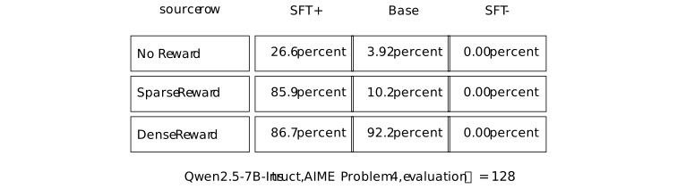
These are source-reported empirical percentages, not exact policy probabilities. ``No Reward'' is retained as the source's row label; the table alone does not define it as a post-training protocol. The three zero entries for SFT-negative are finite observations and remain subject to Remark 6.2.3. Appendix Figure 5's caption prints a different set of Qwen2.5-7B-Instruct values that duplicates the neighbouring movie-quote caption and is incompatible with Table 2. The displayed percentages are those of Table 2; the caption does not provide a consistent alternative measurement.
Remark 6.2.10. An observed plateau is not a universal probability threshold [ftip-00A7]AGENTDRAFTED
Remark 6.2.10. An observed plateau is not a universal probability threshold [ftip-00A7]AGENTDRAFTED
[clay2026demystifying, Section 5.2 and Figure 2] report that the Qwen3-1.7B Base movie-quote cell, whose initial empirical match rate is about 0.5 percent, does not optimize under the source's sparse-reward run, whereas its dense-reward run rises toward fifty percent. [clay2026demystifying, Appendix Figure 8] gives final match rates 10.0 percent for sparse reward and 48.8 percent for dense reward. Thus ``failed'' here means failure of the reported sparse run to optimize as intended, not zero final matches.
A plateau is indexed by the model, target, reward implementation, optimizer, sampling process, and budget in its experiment cell. One observed transition therefore does not identify a universal initial-probability threshold for RL learning, support, or capability acquisition.
6.3. Sparse, dense, and process feedback [ftip-00A8]AGENTDRAFTED
6.3. Sparse, dense, and process feedback [ftip-00A8]AGENTDRAFTED
Sparse, dense, and process rewards expose different observations about a response. This subsection treats that difference as a change in the feedback channel, rather than as a free change in the smoothness of one fixed objective.
Definition 6.3.1. Sparse exact reward [ftip-00A9]AGENTDRAFTED
Definition 6.3.1. Sparse exact reward [ftip-00A9]AGENTDRAFTED
Let \(\mathcal Y\) be a finite response set and fix a target response \(\tau \in \mathcal Y\). The sparse exact reward is the map \(r_{\rm exact}:\mathcal Y\to \{0,1\}\) defined by
\[ r_{\rm exact}(y)=\mathbf 1\{y=\tau \}. \]This idealized reward exposes one bit: whether the whole response equals the target. It does not expose a prefix, edit location, or partial milestone. The movie-quote source uses related but textually inconsistent substring and length-penalized rewards; the distinct formulas are compared in Remark 6.3.2.
Remark 6.3.2. Main-text and Appendix-C sparse-reward discrepancy [ftip-00AA]AGENTDRAFTED
Remark 6.3.2. Main-text and Appendix-C sparse-reward discrepancy [ftip-00AA]AGENTDRAFTED
Section 4.2 of Demystifying Reinforcement Learning Post-Training of Language Models[clay2026demystifying] displays a substring indicator \(\mathbf 1\{\tau \subseteq y\}\) and says that a length penalty is applied. In Appendix C, \(n\) is the maximum generation length and \(s\) is the number of tokens beyond the target. The appendix first defines the excess-length penalty
\[ p(s)= \begin {cases} 0,&s=0,\\ s/n,&s>0, \end {cases} \]and then gives Equation (3):
\[ r_{\rm C}(y,\tau )= \begin {cases} \max \{0.5,1-p(s)\},&\tau \text { occurs in }y \text { and }|y|>|\tau |,\\ 0,&\text {otherwise}. \end {cases} \]As printed, Equation (3) assigns zero when \(y=\tau \), because its first branch requires strict excess length. This conflicts with the immediately preceding Appendix-C prose, which assigns base reward one when the target is generated, and it is not the exact-match reward of Definition 6.3.1. The two printed descriptions therefore specify different reward rules.
Definition 6.3.3. Edit-distance reward [ftip-00AB]AGENTDRAFTED
Definition 6.3.3. Edit-distance reward [ftip-00AB]AGENTDRAFTED
Let \(y=y_1\cdots y_m\) and a nonempty target \(\tau =\tau _1\cdots \tau _n\) be finite strings. Their Levenshtein distance is determined by \(D(0,j)=j\), \(D(i,0)=i\), and, for \(i,j>0\),
\[ D(i,j)=\min \left \{ \begin {aligned} &D(i-1,j)+1,\\ &D(i,j-1)+1,\\ &D(i-1,j-1)+\mathbf 1\{y_i\neq \tau _j\} \end {aligned} \right \}. \]Set \(L(y,\tau )=\max \{|y|,|\tau |\}\). The edit-distance reward is
\[ r_{\rm edit}(y,\tau ) =\max \left \{0,1-\frac {D(|y|,|\tau |)}{L(y,\tau )}\right \}. \]The recurrence is Equation (1) in the main text and Equation (4) in Appendix C of Demystifying Reinforcement Learning Post-Training of Language Models[clay2026demystifying]; the normalized reward is its Equation (5). The nonempty-target assumption makes the displayed denominator positive. This reward does not establish that edit similarity is the correct utility for a different task.
Remark 6.3.4. Dense reward imports target structure [ftip-00AC]AGENTDRAFTED
Remark 6.3.4. Dense reward imports target structure [ftip-00AC]AGENTDRAFTED
The edit reward of Definition 6.3.3 is not obtained from the binary value in Definition 6.3.1 by a numerical smoothing operation. It also receives the target string, a character-level edit model, and the ordering of symbols. Two non-target responses that both receive sparse reward zero can therefore receive different edit rewards.
That extra resolution can improve credit assignment, but it changes the feedback channel and its assumptions. The source calls edit distance a dense proxy and reports controlled movie-quote experiments [clay2026demystifying, Sections 4.2 and 5.2]. Neither the formula nor those observations establish that edit proximity is an independent measure of general response quality.
Definition 6.3.5. Milestone process reward [ftip-00AD]AGENTDRAFTED
Definition 6.3.5. Milestone process reward [ftip-00AD]AGENTDRAFTED
For the source's fixed AIME problem, let
\[ M(y)=(m_1(y),\ldots ,m_5(y))\in \{0,1\}^5 \]record whether a completed response contains five declared milestones: a valid algebraic setup, correct root relations, correct integer bounds, a correct count for at least one branch, and correct subtraction of the overlap at the origin. With
\[ (w_1,\ldots ,w_5)=(0.05,0.05,0.10,0.15,0.25), \]the milestone process reward is
\[ r_{\rm proc}(y)=\sum _{i=1}^{5}w_i m_i(y). \]Appendix D.1 of Demystifying Reinforcement Learning Post-Training of Language Models[clay2026demystifying] gives Equation (6) and the milestone list above. In the experiment, a 32-billion-parameter instruction-tuned model classifies the completed trajectory. The displayed map is therefore richer than a deterministic final-answer verifier, even though it returns one scalar after the rollout.
Remark 6.3.6. Process feedback assumptions and milestone-weight discrepancy [ftip-00AE]AGENTDRAFTED
Remark 6.3.6. Process feedback assumptions and milestone-weight discrepancy [ftip-00AE]AGENTDRAFTED
Appendix D.2 of Demystifying Reinforcement Learning Post-Training of Language Models[clay2026demystifying] supplements \(r_{\rm proc}\) with an extracted-answer override and two penalties. Translating its notation, let \(\tau =117\), \(\tau _{\rm near}=118\), and define
\[ r_{\rm base}(y)= \begin {cases} 1.0,&\operatorname {extract}(y)=\tau ,\\ 0.6,&\operatorname {extract}(y)=\tau _{\rm near},\\ r_{\rm proc}(y),&\text {otherwise}. \end {cases} \]Let \(p_{\rm loop}(y)=-0.3\) when the judge flags a loop without the exact answer, and zero otherwise. Let \(p_{\rm format}(y)=-0.5\) when the response lacks the required boxed delimiter, and zero otherwise. Equations (7)--(8) then give
\[ r_{\rm PRM}(y) =\max \{0,r_{\rm base}(y)+p_{\rm loop}(y)+p_{\rm format}(y)\}. \]These clauses assume a reliable milestone judge, parser, near-miss choice, loop flag, and formatting rule. They are part of the feedback definition, not consequences of reinforcement learning. The main text describes ``exponentially increasing'' dense rewards, and Appendix D calls the weights ``exponential scaling.'' The printed vector \((0.05,0.05,0.10,0.15,0.25)\) is neither strictly increasing at every milestone nor a geometric progression. We preserve the exact weights and do not infer an exponential law from that wording.
Definition 6.3.7. Reward-induced observational equivalence [ftip-00AF]AGENTDRAFTED
Definition 6.3.7. Reward-induced observational equivalence [ftip-00AF]AGENTDRAFTED
Let \(\mathcal Y\) be a finite response set and \(r:\mathcal Y\to \mathcal R\) any reward map. Two responses are observationally equivalent under \(r\), written \(y\sim _r y'\), when
\[ y\sim _r y'\quad \Longleftrightarrow \quad r(y)=r(y'). \]Equality makes \(\sim _r\) an equivalence relation. Its quotient \(\mathcal Y/{\sim _r}\) is the finite set of response classes distinguished by the reward alone. This proposed equivalence relation ignores any information in the response that is not returned by \(r\); equal rewards need not imply equal latent utility.
Lemma 6.3.8. Refining feedback separates at least as many responses [ftip-00AG]AGENTDRAFTED
Lemma 6.3.8. Refining feedback separates at least as many responses [ftip-00AG]AGENTDRAFTED
Let \(\mathcal Y\) be finite and let \(r_1:\mathcal Y\to \mathcal R_1\) and \(r_2:\mathcal Y\to \mathcal R_2\). Say that \(r_2\) refines \(r_1\) when
\[ r_2(y)=r_2(y')\quad \Longrightarrow \quad r_1(y)=r_1(y') \qquad (y,y'\in \mathcal Y). \]If \(r_2\) refines \(r_1\), then
\[ \left |\mathcal Y/{\sim _{r_2}}\right | \geq \left |\mathcal Y/{\sim _{r_1}}\right |. \]
Proof.
Proof.
Send the \(r_2\)-class of \(y\) to the \(r_1\)-class of \(y\). The refinement condition makes this map well defined. It is surjective because every \(r_1\)-class contains some \(y\), whose \(r_2\)-class maps to it. A surjection between finite sets has a domain at least as large as its codomain.
This finite lemma compares observational partitions only. It does not say that the refined reward is cheaper, more accurate, or better aligned with utility.
Example 6.3.9. Counterexample: equal sparse reward, unequal dense reward [ftip-00AH]AGENTDRAFTED
Example 6.3.9. Counterexample: equal sparse reward, unequal dense reward [ftip-00AH]AGENTDRAFTED
Take the target string \(\tau =\texttt {abc}\) and two responses \(y=\texttt {abx}\) and \(y'=\texttt {xyz}\). Both fail exact matching, while their edit distances and normalized edit rewards are
\[ \begin {array}{c|c|c|c} \text {response}&r_{\rm exact}&D(\,cdot\,,\tau )&r_{\rm edit}\\ \hline \texttt {abx}&0&1&2/3\\ \texttt {xyz}&0&3&0 \end {array} \]Thus \(y\sim _{r_{\rm exact}}y'\) but \(y\not \sim _{r_{\rm edit}}y'\). The example witnesses a strict separation inside one sparse-reward class. It does not claim that every dense proxy refines every sparse verifier.
Example 6.3.10. Three feedback resolutions on one response set [ftip-00AI]AGENTDRAFTED
Example 6.3.10. Three feedback resolutions on one response set [ftip-00AI]AGENTDRAFTED
One finite response set can be observed through three different maps. The arrows below share a domain; they do not assert that the three codomains form a refinement chain.
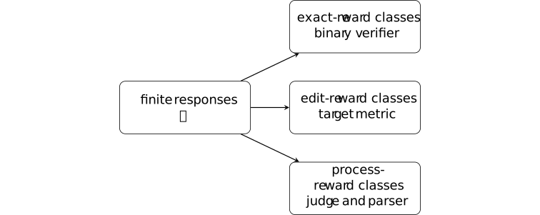
The exact reward forgets every difference among failures. Edit reward can retain character-level proximity, while the source process reward retains a declared milestone vector only after judge, override, and penalty choices. The partition lemma Lemma 6.3.8 applies to a pair only after its refinement hypothesis has been checked.
Remark 6.3.11. Reward density is not cost-free smoothing [ftip-00AJ]AGENTDRAFTED
Remark 6.3.11. Reward density is not cost-free smoothing [ftip-00AJ]AGENTDRAFTED
A denser reward can distinguish more responses and supply more frequent update signal. It can also require information absent from a sparse verifier. In the controlled source, edit feedback assumes the full target and computes a string metric; process feedback uses a 32-billion-parameter judge, five problem-specific milestones, answer extraction, an enumerated near miss, and loop and format penalties [clay2026demystifying, Appendices C--D].
The richer feedback channel incurs specification, computation, and validation costs. Replacing sparse feedback by dense feedback can alter both the information available to training and the objective being optimized. The resulting comparison is an intervention on feedback resolution, not evidence that one fixed reward was smoothed at zero cost.
6.4. Prompt breadth and effect locality [ftip-00AK]AGENTDRAFTED
6.4. Prompt breadth and effect locality [ftip-00AK]AGENTDRAFTED
Training on one prompt law can change behavior unevenly across evaluation slices. Localized and distributed degradation are distinguished relative to that training law and the specified evaluation slices.
Definition 6.4.1. Training prompt law and evaluated prompt slice [ftip-00AL]AGENTDRAFTED
Definition 6.4.1. Training prompt law and evaluated prompt slice [ftip-00AL]AGENTDRAFTED
Let \(\mathcal X\) be a task-instance set. Write \(\mu _{\rm tr}=\mathcal D_{\rm tr}\) for the training-prompt coordinate of an experiment cell in Definition 6.1.6. A training prompt law is this probability law on \(\mathcal X\), used to draw instances during a post-training protocol. Let \(\mu _{\rm ev}\) be an independently declared evaluation law on the same set.
An evaluated prompt slice is a measurable set \(C\subseteq \mathcal X\) with \(\mu _{\rm ev}(C)>0\). Its conditional evaluation law is
\[ \mu _{\rm ev}(A\mid C) =\frac {\mu _{\rm ev}(A\cap C)}{\mu _{\rm ev}(C)}. \]The training and evaluation laws need not agree. A slice records where an effect is measured; it does not assert that prompts inside the slice are equally difficult or represented equally in pretraining. We specialize the task-law convention of Definition [ftip-001Q].
Definition 6.4.2. Source-specific narrow and broad configurations [ftip-00AM]AGENTDRAFTED
Definition 6.4.2. Source-specific narrow and broad configurations [ftip-00AM]AGENTDRAFTED
A prompt configuration is the record
\[ \mathsf c=(M_0,\mu _{\rm tr},m_{\rm tr},r,\mathsf A,b), \]containing the starting artifact, training prompt law, finite prompt-pool size, reward, update algorithm, and training budget. We call two particular records \(\mathsf c_{\rm nar}\) and \(\mathsf c_{\rm brd}\) only when a cited experiment names them narrow and broad.
Section 4.3 and Appendix F of Demystifying Reinforcement Learning Post-Training of Language Models[clay2026demystifying] instantiate these labels in two model-family experiments. The Qwen comparison uses 100 DeepScaleR prompts versus 10,000 WildChat prompts. The OLMo comparison uses 100 math-only prompts versus 10,000 prompts split evenly among mathematics, instruction following, and code. These labels identify the two reported configurations; they do not define a general measure or ordering of prompt breadth.
Remark 6.4.3. Prompt breadth is not a total order [ftip-00AN]AGENTDRAFTED
Remark 6.4.3. Prompt breadth is not a total order [ftip-00AN]AGENTDRAFTED
The records in Definition 6.4.2 change several coordinates together. The prompt-pool size, domain mixture, and repetition frequency differ. Across the paper's Qwen and OLMo studies, the starting artifact and evaluated tasks also differ.
We therefore use ``narrow'' and ``broad'' as names for the source cells. They do not define a total order on prompt laws, and their comparison does not identify a causal effect of breadth alone. A breadth theorem would need a declared statistic and matched configurations that differ only in that statistic.
Definition 6.4.4. Slice-conditioned success change [ftip-00AO]AGENTDRAFTED
Definition 6.4.4. Slice-conditioned success change [ftip-00AO]AGENTDRAFTED
Fix an evaluated slice \(C\) from Definition 6.4.1, and let \(P_0\) and \(P_1\) denote the pre- and post-training protocols whose successful-support probabilities are defined in Definition 3.1. The slice-conditioned success change is
\[ \Delta _{\rm suc}(C;P_1,P_0) =\mathbb E_{X\sim \mu _{\rm ev}(\cdot \mid C)} \left [p_{P_1}(X)-p_{P_0}(X)\right ]. \]The evaluation interface, inference budget, and success predicate are held fixed across the two terms. The quantity is an average change on one declared slice. It neither locates the change inside the model nor identifies which training coordinate caused it.
Definition 6.4.5. Localized and distributed degradation [ftip-00AP]AGENTDRAFTED
Definition 6.4.5. Localized and distributed degradation [ftip-00AP]AGENTDRAFTED
Fix pairwise disjoint evaluated slices \(C_1,\ldots ,C_J\) and a declared degradation threshold \(\kappa >0\). Define the set of materially degraded slices
\[ \mathcal H_\kappa (P_1,P_0) =\left \{j:\Delta _{\rm suc}(C_j;P_1,P_0)\leq -\kappa \right \}. \]Degradation is localized relative to this slice family and threshold when \(|\mathcal H_\kappa |=1\). It is distributed when \(|\mathcal H_\kappa |\geq 2\).
These terms depend on the chosen partition, threshold, and evaluation budget. They do not turn a finite benchmark vector into a statement about all capabilities.
Example 6.4.6. Narrow and broad random-reward paths [ftip-00AQ]AGENTDRAFTED
Example 6.4.6. Narrow and broad random-reward paths [ftip-00AQ]AGENTDRAFTED
Section 5.3 and Appendix F of Demystifying Reinforcement Learning Post-Training of Language Models[clay2026demystifying] supply two OLMo paths; Figure 4 reports their outcomes. Both replace the usual verifiable reward with a random scalar drawn from \(\operatorname {Unif}[0,1]\), but their prompt configurations differ.
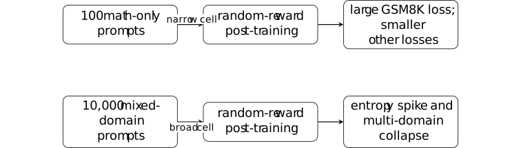
In the narrow SFT-start path, GSM8K accuracy falls from 86 to about 32 by step 400, while the reported MMLU and IFEval changes are much smaller. In the broad path, the source reports an entropy spike near step 400 together with collapse on GSM8K, MMLU, and IFEval. The diagram records that interpretation; it does not isolate prompt breadth from pool size, mixture, or repetition.
Remark 6.4.7. What the source observes about spurious reward [ftip-00AR]AGENTDRAFTED
Remark 6.4.7. What the source observes about spurious reward [ftip-00AR]AGENTDRAFTED
Section 5.3 and Figures 3--4 of Demystifying Reinforcement Learning Post-Training of Language Models[clay2026demystifying] report that the Qwen narrow configuration retains higher MATH and AMC Acc@1 than its broad configuration under random reward. The OLMo experiment reports the different evaluation patterns summarized in Example 6.4.6.
These are finite empirical observations. The random scalar reward removes task alignment from one feedback channel, but it does not hold all other training coordinates fixed. The reported entropy is a named token statistic, not a direct measure of capability or acquisition.
Example 6.4.8. Counterexample: equal marginal reward, unequal prompt-local damage [ftip-00AS]AGENTDRAFTED
Example 6.4.8. Counterexample: equal marginal reward, unequal prompt-local damage [ftip-00AS]AGENTDRAFTED
Let two evaluation slices \(C_1,C_2\) have equal mass. A feedback channel returns an independent Bernoulli reward with mean \(1/2\) under either of two post-training protocols. Suppose their fixed-interface success changes are
\[ \left (\Delta _{\rm suc}(C_1),\Delta _{\rm suc}(C_2)\right ) =(-1,0) \quad \hbox {or}\quad \left (-\tfrac 12,-\tfrac 12\right ). \]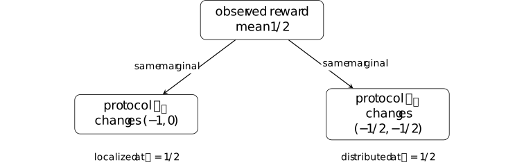
The reward law and its mean are identical, but the slice-level evaluation vectors differ. Hence marginal training reward does not determine whether damage is localized or distributed. This is a finite counterexample, not a claim about the mechanism in the source experiment.
Remark 6.4.9. Coverage, feedback resolution, and prompt-conditioned effects [ftip-00AT]AGENTDRAFTED
Remark 6.4.9. Coverage, feedback resolution, and prompt-conditioned effects [ftip-00AT]AGENTDRAFTED
The source cells motivate tests of starting-policy coverage, feedback resolution, and prompt-conditioned damage. They do not establish that dense reward creates mathematical support, that zero sampled hits imply zero probability, or that random reward has one model-independent effect.
Separating the effects of coverage, feedback resolution, and prompt breadth requires stronger controls. One comparison fixes prompt laws and varies only the feedback sigma-algebra. Another fixes feedback and evaluation while varying one starting-policy coordinate. Confidence regions for the complete vector of slice-conditioned changes would quantify effects that an aggregate score can hide.
The reported observations remain conditional on their experimental configurations. They do not establish general results about capability acquisition, elicitation, or the optimal allocation of post-training compute.
7. Finite consequences and counterexamples [ftip-00JE]AGENTDRAFTED
7. Finite consequences and counterexamples [ftip-00JE]AGENTDRAFTED
Finite sampling, reward information, and deterministic execution give conditional conclusions about post-training. Their counterexamples show why the task law, feasible set, and available information cannot be omitted.
This synthesis brings together the finite results used in the evaluation analysis. The conceptual-discovery chapter asks whether such arguments can constrain a complete learning lineage, including changes to representations, curricula and research procedures.
7.1. Probability, information, and execution [ftip-00I1]AGENTDRAFTED
7.1. Probability, information, and execution [ftip-00I1]AGENTDRAFTED
Discovery probabilities, support, proxy error, feedback resolution, and replay each constrain a different part of a comparison. Capability remains conditional behavior under a declared intervention and evaluation law, rather than a scalar latent property.
7.1.1. Finite probability and execution results [ftip-00I2]AGENTDRAFTED
7.1.1. Finite probability and execution results [ftip-00I2]AGENTDRAFTED
The conclusions depend on their declared probability laws, finite index sets, positivity conditions, and execution inputs. Changing one of these assumptions can change the result even when the observed score is unchanged.
Convention 7.1.1.1. Domains of the finite results [ftip-00I5]AGENTDRAFTED
Convention 7.1.1.1. Domains of the finite results [ftip-00I5]AGENTDRAFTED
Each result concerns its declared carriers \(X_1,\ldots ,X_n\), with fixed equality and order conventions. Finiteness, probability laws, and positivity conditions are hypotheses of the result; they cannot be inferred from a finite observation alone.
Theorem 7.1.1.2. Independent discovery probability [ftip-00I7]AGENTDRAFTED
Theorem 7.1.1.2. Independent discovery probability [ftip-00I7]AGENTDRAFTED
For \(B\in \mathbb N\) independent discovery events with the probabilities declared in Convention 4.1.1, the identity in Theorem 4.1.2 gives \(\Pr (D_B)=1-\prod _{i=1}^{B}(1-p_i)\).
Theorem 7.1.1.3. Discovery budget for a failure threshold [ftip-00I8]AGENTDRAFTED
Theorem 7.1.1.3. Discovery budget for a failure threshold [ftip-00I8]AGENTDRAFTED
Under \(0<p<1\), \(0<\delta <1\), and an integer budget \(B\geq 1\), the failure constraint is equivalent to the following bound.
\[B\geq \left \lceil \frac {\log \delta }{\log (1-p)}\right \rceil .\]The result is proved in Corollary 4.1.3.
Theorem 7.1.1.4. Support under finite exponential tilting [ftip-00I9]AGENTDRAFTED
Theorem 7.1.1.4. Support under finite exponential tilting [ftip-00I9]AGENTDRAFTED
Under the finite-carrier and positive-temperature hypotheses of Theorem 4.1.6, normalized exponential tilting preserves the base law's positive support.
Theorem 7.1.1.5. Uniform proxy error and objective regret [ftip-00IA]AGENTDRAFTED
Theorem 7.1.1.5. Uniform proxy error and objective regret [ftip-00IA]AGENTDRAFTED
For a finite common feasible set and a common regularizer, the uniform proxy error hypothesis in Definition 4.2.1 yields the two-epsilon objective regret bound proved in Theorem 4.2.2; the conclusion concerns the regularized objective named there.
Theorem 7.1.1.6. Utility under a change of evaluation law [ftip-00IB]AGENTDRAFTED
Theorem 7.1.1.6. Utility under a change of evaluation law [ftip-00IB]AGENTDRAFTED
If the evaluation laws and finite response space satisfy the total-variation hypotheses of Theorem 2.5.2, then the expectation difference is bounded by the stated sup-norm times total variation.
Theorem 7.1.1.7. Response classes under feedback refinement [ftip-00IC]AGENTDRAFTED
Theorem 7.1.1.7. Response classes under feedback refinement [ftip-00IC]AGENTDRAFTED
For finite response set \(\mathcal Y\) and deterministic rewards, a reward channel that refines the equality partition of another channel separates at least as many response classes, as proved in Lemma 6.3.8.
Theorem 7.1.1.8. Equal execution inputs give equal replay traces [ftip-00IJ]AGENTDRAFTED
Theorem 7.1.1.8. Equal execution inputs give equal replay traces [ftip-00IJ]AGENTDRAFTED
If the execution map is deterministic in all coordinates fixed by Definition [ftip-00HF], then equal input, revision, environment, and seed records produce equal finite traces, as proved in Theorem [ftip-00HG].
Theorem 7.1.1.9. Observational equivalence under a common update kernel [ftip-00IK]AGENTDRAFTED
Theorem 7.1.1.9. Observational equivalence under a common update kernel [ftip-00IK]AGENTDRAFTED
For the finite transcript and world kernels declared in Definition 4.3.2--Definition 4.3.3, observationally equivalent worlds induce the same output law for any common randomized post-training kernel, as proved in Theorem 4.3.5.
Theorem 7.1.1.10. Conditions for an admissible commit decision [ftip-00IL]AGENTDRAFTED
Theorem 7.1.1.10. Conditions for an admissible commit decision [ftip-00IL]AGENTDRAFTED
Under the typed audit record of Definition [ftip-00HL], a commit is admissible exactly when all required checks pass, the digest matches, and the recorded decision is \(commit\), as proved in Theorem [ftip-00HM].
Theorem 7.1.1.11. Admission of a finite audit plan [ftip-00IM]AGENTDRAFTED
Theorem 7.1.1.11. Admission of a finite audit plan [ftip-00IM]AGENTDRAFTED
A finite audit plan with nonnegative stage costs is admissible exactly when its declared additive cost is within budget; adding a positive stage beyond slack is inadmissible, by Theorem [ftip-00HX].
7.1.2. Counterexamples and restricted assumptions [ftip-00ID]AGENTDRAFTED
7.1.2. Counterexamples and restricted assumptions [ftip-00ID]AGENTDRAFTED
Finite constructions can separate average success from coverage, proxy accuracy from evaluation quality, and observed gradients from the hypotheses needed to bound them. Each separation identifies an assumption that a stronger conclusion would require.
Remark 7.1.2.1. What a finite counterexample establishes [ftip-00IE]AGENTDRAFTED
Remark 7.1.2.1. What a finite counterexample establishes [ftip-00IE]AGENTDRAFTED
A finite assignment satisfying a claim's hypotheses and violating its conclusion disproves that universal claim. It does not estimate how often the failure occurs under another distribution or establish a general failure rate.
Remark 7.1.2.2. Changing the model or evaluation changes the claim [ftip-00IF]AGENTDRAFTED
Remark 7.1.2.2. Changing the model or evaluation changes the claim [ftip-00IF]AGENTDRAFTED
A conclusion about fixed carriers, policies, feedback, budgets, and evaluation laws need not survive a change to those objects. Finite zero hits do not imply zero support, empirical benchmark movement does not imply acquisition, and an exact-optimizer result need not hold for an approximate optimizer without an additional error bound.
Example 7.1.2.3. Equal averages and zero hits do not identify coverage [ftip-00IG]AGENTDRAFTED
Example 7.1.2.3. Equal averages and zero hits do not identify coverage [ftip-00IG]AGENTDRAFTED
The two-task examples in Example 4.1.8 and Example 6.2.6 show that equal one-shot averages or zero observed hits can coexist with different coverage or nonzero latent rates. These conclusions use their declared iid model and do not estimate rates outside it.
Example 7.1.2.4. Small training-law error can reverse evaluation selection [ftip-00IH]AGENTDRAFTED
Example 7.1.2.4. Small training-law error can reverse evaluation selection [ftip-00IH]AGENTDRAFTED
In the two-point construction of Example 4.2.4, training-law average error is small while evaluation selection reverses. The missing hypothesis is a uniform bound on the evaluated feasible set; an informal promise of similar distributions does not supply it.
Remark 7.1.2.5. Untied heads, shared gradients, and checkpoint forecasts [ftip-00II]AGENTDRAFTED
Remark 7.1.2.5. Untied heads, shared gradients, and checkpoint forecasts [ftip-00II]AGENTDRAFTED
For DGG, the untied head identity and its finite-batch Jensen bound in Theorem 4.4.1 and Theorem 4.4.3 differ from an intermediate-occurrence bound. A shared intermediate weight requires the sum over all occurrences in Theorem 4.4.1; the source's local hypotheses do not establish its claimed total-gradient bound in [miao2026when, Section 4.2.1, Lemma 1, Theorem 1, and Appendix A.3]. The cancellation example Example 4.4.6 also separates the active clipping interval from the raw-surrogate extension.
NExt's empirical checkpoint forecasts in [chen2026lowrank, Sections 3.2, 4.1--4.3, and 5.1] do not establish a universal subspace-collapse, capability, or speed theorem. The spectral and evaluation quantities in Definition 4.4.8 through Remark 4.4.13 measure different trajectory properties.
7.1.3. Mathematical notation [ftip-00IN]AGENTDRAFTED
7.1.3. Mathematical notation [ftip-00IN]AGENTDRAFTED
Prompt and response spaces, probability laws, policies, rewards, evaluation scores, and execution traces are distinct mathematical objects.
Convention 7.1.3.1. Prompt spaces, response spaces, and laws [ftip-00IO]AGENTDRAFTED
Convention 7.1.3.1. Prompt spaces, response spaces, and laws [ftip-00IO]AGENTDRAFTED
Use \(\mathcal X\) for prompts, \(\mathcal Y\) for finite responses, \(\Omega \) for sample space, \(\mathsf P\) for a declared protocol, and \(\mu \) for a prompt law. A probability law is written \(\Pr \) only after its sample space is named.
Convention 7.1.3.2. Policies and reference policies [ftip-00IP]AGENTDRAFTED
Convention 7.1.3.2. Policies and reference policies [ftip-00IP]AGENTDRAFTED
Use \(\pi \) for a policy, \(\pi _{\rm base}\) for a reference policy, and \(\pi _\theta \) for a parameterized policy. A policy is always typed as a kernel from the declared prompt carrier to the declared response carrier.
Convention 7.1.3.3. Rewards and evaluation utilities [ftip-00IQ]AGENTDRAFTED
Convention 7.1.3.3. Rewards and evaluation utilities [ftip-00IQ]AGENTDRAFTED
Use \(r:\mathcal X\times \mathcal Y\to \mathbb R\) for a deterministic reward and \(u\) for an evaluation utility. Proxy, verifier, and process rewards retain their local subscripts; no bare symbol silently changes meaning.
Convention 7.1.3.4. Model artifacts and evaluation scores [ftip-00IR]AGENTDRAFTED
Convention 7.1.3.4. Model artifacts and evaluation scores [ftip-00IR]AGENTDRAFTED
Use \(M\) for a model artifact, \(\mathsf E\) for an evaluation protocol, and \(J_{\mathsf E}(M)\) for its declared score. A comparison must state the invariant evaluation law before subtracting two scores.
Convention 7.1.3.5. Traces, states, lineages, and costs [ftip-00IS]AGENTDRAFTED
Convention 7.1.3.5. Traces, states, lineages, and costs [ftip-00IS]AGENTDRAFTED
Use \(z_{0:n}\) for a finite trace, \(s_t\) for a harness state, \(\ell \) for a lineage, and \(c\) for an execution cost. Event logs and summaries are distinct carriers even when one is computed from the other.