Compact gauge groups and representation data [fdip-007A]
✍️sourceAGENTDRAFTED
- November 1, 2026
Compact gauge groups and representation data [fdip-007A]
✍️sourceAGENTDRAFTED
- November 1, 2026
Replacing a finite gauge group by a compact group changes edge sums into normalized Haar integrals. Character orthogonality survives, but an infinite character expansion needs a convergence argument before it can be inserted into a surface partition function. The distinction between an \(L^2\) expansion and an absolutely convergent kernel is therefore part of the model.
For the circle group, Wilson and Villain weights give explicit Fourier coefficients. Matching one coefficient does not match the whole law. For matrix groups, a separate smooth-field calculation explains the classical small-spacing normalization of the Wilson action. Neither calculation constructs a quantum continuum limit.
Unit quaternions identify the compact group \(SU(2)\) and its binary polyhedral subgroups. A representation datum then specifies which group acts on which field and whether it also moves the substrate. These choices precede any physical comparison.
Theorem 1. Normalized Haar measure [fdip-007B]AGENTDRAFTED
- November 1, 2026
Theorem 1. Normalized Haar measure [fdip-007B]AGENTDRAFTED
- November 1, 2026
Every compact Hausdorff topological group \(G\) has a unique regular Borel probability measure \(\mu _G\) invariant under left translation. This is the normalized Haar theorem, used here as a cited statement; existence and uniqueness are not proved in these notes. The existence and uniqueness-up-to-scale statements are Theorems 4.3 and 4.6 in [gleason2010haar, pp. 6, 11]. Compactness permits normalization to total mass one.
The normalized measure is also invariant under right translation and inversion. Indeed, a right translate of \(\mu _G\) is another left-invariant regular probability measure, hence equals \(\mu _G\) by uniqueness. The pushforward under inversion is then left invariant, because inversion changes left translations into right translations; it too has total mass one and equals \(\mu _G\). These deductions explain why the same measure works with either orientation of an edge.
Every nonempty open set has positive Haar measure. If an open set had measure zero, choose a point in it; its left translates cover \(G\), and compactness gives a finite subcover, contradicting total mass one. Consequently a continuous function that vanishes \(\mu _G\)-almost everywhere vanishes everywhere.
For a finite group this measure is uniform counting. For \(U(1)=\{e^{i\theta }:\theta \in \mathbb R\}\), it is \(d\theta /(2\pi )\) on one period: translation invariance and total mass one identify this measure by uniqueness. Product Haar measure on the edge space \(G^E\) supplies the compact measure assumed in the joint matter law. For \(U(1)\) and \(SU(2)\), all spaces here are compact metrizable, so their Borel products have the usual product measurable structure.
Mathlib constructs Haar measure as
MeasureTheory.Measure.haarMeasure, normalized on a chosen
compact set with nonempty interior; for compact \(G\), choose that
set to be all of \(G\). The separate declaration
MeasureTheory.Measure.isHaarMeasure_eq_of_isProbabilityMeasure
asserts equality of two Haar probability measures on a locally compact
topological group with its Borel measurable structure. It has no
second-countability assumption. These are correspondences for the
construction and normalized uniqueness, respectively; the right and
inversion invariance arguments above are stated separately.
Theorem 2. Compact character expansions and surface integrals [fdip-007C]AGENTDRAFTED
- November 1, 2026
Theorem 2. Compact character expansions and surface integrals [fdip-007C]AGENTDRAFTED
- November 1, 2026
Let \(G\) be a compact Lie group with normalized Haar measure. Choose unitary representatives of its complex irreducibles, indexed by \(\widehat G\), with dimensions \(d_\rho \). The Peter–Weyl theorem says that the functions \(\sqrt {d_\rho }\rho (\cdot )_{ij}\) form an orthonormal basis of \(L^2(G)\). Its central subspace has orthonormal basis \(\chi _\rho \). Thus a central \(f\in L^2(G)\) has the expansion \[f=\sum _{\rho \in \widehat G}c_\rho \chi _\rho , \qquad c_\rho =\int _G f(h)\overline {\chi _\rho (h)}\,d\mu _G(h),\] with convergence in \(L^2\). This is a cited statement, namely Woit's Section 5, Theorem 1 and Corollary 1 [woit2012peterweyl, p. 6]. It does not assert pointwise or absolute convergence for an arbitrary \(L^2\) function.
For an inequivalent exhaustive family of finite-dimensional unitary
continuous models, TauCeti's
TauCeti.peterWeylBasis constructs the normalized
matrix-coefficient Hilbert basis, with its inner-product convention
for matrix coefficients. Over \(\mathbb C\), its coefficient
\(\langle \rho (g)e_a,e_b\rangle \) is the conjugate of the matrix
entry \(\rho (g)_{ba}\); conjugation, or reindexing by dual
representations, gives the equivalent entry-coordinate basis.
The separate TauCeti.characterBasis constructs
the actual character basis of the central \(L^2\) subspace.
Compact Hausdorff groups over \(\mathbb C\), hence the compact Lie
groups here, satisfy the stated hypotheses. These correspondences
support the two \(L^2\) basis statements, not the uniform absolute
convergence or surface integral established next.
Suppose now that \(f\) is continuous and central and that \[\sum _{\rho \in \widehat G}|c_\rho |d_\rho <\infty .\] Then its character expansion converges uniformly and absolutely. For the closed oriented polygonal surface, with \(P\) faces and genus \(g\), define the edge integral \[Z_\Sigma (f)=\int _{G^E}\prod _p f(U_p)\,d\mu (U).\] Under the displayed summability condition, \[Z_\Sigma (f)=\sum _{\rho \in \widehat G} d_\rho ^{2-2g}\left (\frac {c_\rho }{d_\rho }\right )^P,\] and this numerical series is absolutely convergent.
Proof.
- November 1, 2026
Proof.
- November 1, 2026
Unitarity gives \(|\chi _\rho (h)|\le d_\rho \). The sum of the uniform bounds is finite, so the character series has a continuous uniform limit. Peter–Weyl identifies that limit with \(f\) in \(L^2\); continuity and full support of Haar measure make the equality pointwise. Expanding a product over the finite face set gives a sum whose total absolute value is bounded uniformly by \[\left (\sum _\rho |c_\rho |d_\rho \right )^P.\] This bound is integrable against probability measure, justifying interchange of the full face-label sum and the edge integrals.
Haar averaging gives the same matrix orthogonality as finite averaging: for \(A:V_\tau \to V_\rho \), the integral \(\int _G\rho (h)A\tau (h)^{-1}\,d\mu _G(h)\) is an intertwiner. Schur's lemma and its trace make it zero for inequivalent representatives and \((\operatorname {tr}A/d_\rho )I\) for equal ones. The edge contractions and circular vertex links in the finite surface proof therefore leave one common face label and one free index per vertex. Their contribution is \(c_\rho ^P d_\rho ^{|V|-|E|}\), the displayed formula. Absolute convergence follows as well: the absolute values of these integrated terms are bounded by the integrals of the absolute face terms, whose total has just been bounded. In particular \(f=1\) still gives \(Z_\Sigma (1)=1\).
Definition 3. Convolution kernels with positive coefficients [fdip-007I]AGENTDRAFTED
- November 1, 2026
Definition 3. Convolution kernels with positive coefficients [fdip-007I]AGENTDRAFTED
- November 1, 2026
For a finite or compact Lie group \(G\), use the normalized Haar measure, irreducibles and dimensions of the character expansion. For convolution constructions, consider real continuous central kernels \(k\) with the separate hypotheses \[\begin {gathered} k(h)>0,\qquad k(h^{-1})=k(h),\\ k(h)=\sum _{\rho \in \widehat G}d_\rho a_\rho \chi _\rho (h), \qquad a_\rho >0,\qquad \sum _{\rho \in \widehat G}d_\rho ^2a_\rho <\infty . \end {gathered}\] The last condition gives uniform absolute convergence; inversion symmetry and reality impose the corresponding agreement of conjugate coefficients. The convention is \(c_\rho =d_\rho a_\rho \), not \(c_\rho =a_\rho \). These are assumptions on a kernel, not consequences of the Peter–Weyl theorem. In particular, pointwise positivity does not imply the coefficient condition, as the circle counterexample shows.
Example 4. A positive weight with a negative coefficient [fdip-007J]AGENTDRAFTED
- November 1, 2026
Example 4. A positive weight with a negative coefficient [fdip-007J]AGENTDRAFTED
- November 1, 2026
On \(U(1)\), take \(0<\epsilon <1\) and \[k(e^{i\theta })=1-\epsilon \cos \theta =1-\frac \epsilon 2 e^{i\theta }-\frac \epsilon 2 e^{-i\theta }.\] This is a real continuous central function, unchanged by inversion, and \(k\ge 1-\epsilon >0\). Its character coefficients at \(n=\pm 1\) are nevertheless \(-\epsilon /2\). Thus the pointwise and Fourier positivity assumptions in the kernel definition are distinct.
Proposition 5. Wilson and Villain coefficients on the circle [fdip-007D]AGENTDRAFTED
- November 1, 2026
Proposition 5. Wilson and Villain coefficients on the circle [fdip-007D]AGENTDRAFTED
- November 1, 2026
For \(G=U(1)\), use characters \(\chi _n(e^{i\theta })=e^{in\theta }\) with \(n\in \mathbb Z\) and normalized Haar measure \(d\theta /(2\pi )\). For \(\beta >0\), the Wilson weight \(w_\beta (\theta )=e^{\beta \cos \theta }\) has coefficients \[I_n(\beta )=\sum _{j=0}^\infty \frac {(\beta /2)^{2j+|n|}}{j!(j+|n|)!}>0, \qquad \sum _{n\in \mathbb Z}I_n(\beta )=e^\beta .\] Thus its character series is uniformly absolutely convergent. The Wilson action convention includes the additional constant factor \(e^{-\beta }\); this multiplies all coefficients but cancels from the normalized one-plaquette probability.
TauCeti's
Real.integral_exp_mul_cos_mul_cexp
proves the Wilson circle integral with exponent \(+in\theta \) and
unnormalized measure on \([-\pi ,\pi ]\). Replacing \(n\) by \(-n\)
and dividing by \(2\pi \) gives the coefficient convention here;
its Bessel value has the displayed power series. This correspondence
supports the Wilson coefficient identity, not the Villain formula
or the comparison of the two weights.
For \(\beta _V>0\), the Villain weight is the periodic Gaussian \[v_{\beta _V}(\theta )=\sum _{\ell \in \mathbb Z} \exp \left [-\frac {\beta _V}{2}(\theta -2\pi \ell )^2\right ].\] Its character coefficient is \[c_n^V=(2\pi \beta _V)^{-1/2} e^{-n^2/(2\beta _V)}.\] The coefficient series is again uniformly absolutely convergent and all coefficients are strictly positive. Dividing each weight by its zeroth coefficient normalizes its integral to one, giving \[\widehat c_n^W=\frac {I_n(\beta )}{I_0(\beta )},\qquad \widehat c_n^V=e^{-n^2/(2\beta _V)}.\] These normalized coefficients differ from the unnormalized \(c_\rho \) in the surface formula.
Proof.
- November 1, 2026
Proof.
- November 1, 2026
Put \(z=e^{i\theta }\). Multiply the two absolutely convergent series for \(\exp (\beta z/2)\) and \(\exp (\beta z^{-1}/2)\). The coefficient of \(z^n\) is the displayed \(I_n\); the total of all absolute coefficients is the product \(e^{\beta /2}e^{\beta /2}\). Every \(I_n\) is positive for \(\beta >0\).
For the periodic Gaussian, uniform Gaussian tail bounds on a period justify continuity and integration term by term. Unfolding its coefficient integral gives \[c_n^V=\frac 1{2\pi }\int _{\mathbb R} e^{-\beta _V x^2/2}e^{-inx}\,dx.\] For real \(t\), let \(J(t)\) be the integral without \(1/(2\pi )\) and with \(n\) replaced by \(t\). Gaussian domination permits differentiation under the integral. Integration by parts, with vanishing boundary terms, gives \(J'(t)=-(t/\beta _V)J(t)\). Since \(J(0)=\sqrt {2\pi /\beta _V}\), this proves the coefficient formula. The Gaussian coefficient bound is summable over \(n\). Its uniformly convergent Fourier series has the same coefficients as the continuous periodic Gaussian, so completeness of the character basis and continuity identify the two functions. Finally, the integral of a weight is its zeroth coefficient, which proves the normalization.
Both positive-parameter weights satisfy the positive-character kernel hypotheses: they are real, strictly positive, invariant under inversion, and have positive summable coefficients. For \(U(1)\) every irreducible dimension is one. This checks the kernel assumptions without asserting any transfer-operator or continuum conclusion.
Theorem 6. The matched Wilson and Villain laws differ [fdip-007E]AGENTDRAFTED
- November 2, 2026
Theorem 6. The matched Wilson and Villain laws differ [fdip-007E]AGENTDRAFTED
- November 2, 2026
A single \(U(1)\) plaquette has the normalized Wilson or Villain weight. Matching their fundamental Fourier coefficients determines a Villain coupling for every Wilson coupling. The two probability laws still differ.
For \(\beta >0\), write \(r(\beta )=I_1(\beta )/I_0(\beta )\) and \(\beta _V(\beta )=-\frac {1}{2\log r(\beta )}\). Then \(0<r(\beta )<1\), the matched Villain coefficient is \(r(\beta )^{n^2}\), and \[\frac {\widehat c_n^W}{\widehat c_n^V}\to \infty \] as \(|n|\to \infty \). In particular the two normalized weights are distinct, so they define distinct probability laws on the circle. The second Wilson coefficient is \(1-\frac {2r(\beta )}{\beta }\).
Proof.
- November 2, 2026
Proof.
- November 2, 2026
The series for \(I_1\) has positive terms, so \(r>0\). With normalized Haar measure, \[\int (1-\cos \theta )\,e^{\beta \cos \theta }\,\frac {d\theta }{2\pi } =I_0(\beta )-I_1(\beta ).\] The integrand is nonnegative and not identically zero, and the exponential is positive, so the integral is positive. Thus \(r<1\), the logarithm is negative, and \(\beta _V\) is positive. The Villain normalization in the coefficient note gives \(\widehat c_n^V=\exp (-n^2/(2\beta _V))\). Substituting the displayed \(\beta _V\) produces \(1/(2\beta _V)=-\log r\), hence \(\widehat c_n^V=r^{n^2}\).
The \(j=0\) term of the series for \(I_n(\beta )\), with \(n\ge 0\), is \((\beta/2)^n/n!\). Every term is positive, so \(I_n(\beta )\ge (\beta/2)^n/n!\). Therefore \(\widehat c_n^W=I_n(\beta )/I_0(\beta )\) satisfies \[\frac {\widehat c_n^W}{r^{n^2}} \ge \frac {(\beta/2)^n}{n!\,I_0(\beta )\,r^{n^2}}.\] For \(n\ge 1\), one has \(n!\le n^n\), so the logarithm of the right-hand side is at least \(n\log (\beta/2)-n\log n-\log I_0(\beta )-n^2\log r\). The last summand tends to \(+\infty \) because \(\log r<0\), and it dominates the remaining terms. The lower bound tends to infinity, and so does the ratio, as \(n\to +\infty \). The series in the coefficient note depends on \(|n|\), so \(I_n(\beta )=I_{-n}(\beta )\). The matched Villain coefficient \(r^{n^2}\) is likewise unchanged when \(n\) is replaced by \(-n\). The ratio at \(-n\) equals the ratio at \(n\), and the same limit holds as \(|n|\to \infty \).
The coefficient note identifies each normalized continuous weight with its Fourier series. Some coefficient of large order differs, so the weights differ as functions and as probability laws.
The same series gives the second coefficient. The identity \(\frac {2}{\beta }(\beta/2)^{2j+1}=(\beta/2)^{2j}\) rewrites \[\frac {2}{\beta }I_1(\beta ) =\sum _{j\ge 0}\frac {(\beta/2)^{2j}}{j!\,(j+1)!}.\] Subtracting from \(I_0\) cancels the \(j=0\) term. For \(j\ge 1\) the difference of the summands is \(\frac {(\beta/2)^{2j}\,j}{j!\,(j+1)!} =\frac {(\beta/2)^{2j}}{(j-1)!(j+1)!}\), which is the \(j-1\) term of \(I_2\). Hence \(I_0-I_2=\frac {2}{\beta }I_1\), and \(\widehat c_2^W=1-\frac {2r(\beta )}{\beta }\). At \(\beta =2\) this coefficient is \(1-r(2)\), while the matched Villain coefficient is \(r(2)^4\).
The comparison is a one-plaquette identity. It does not assert a many-plaquette continuum limit.
Proposition 7. The classical small-spacing Wilson action [fdip-007F]AGENTDRAFTED
- November 1, 2026
Proposition 7. The classical small-spacing Wilson action [fdip-007F]AGENTDRAFTED
- November 1, 2026
Fix a flat \(d\)-dimensional torus with \(d\ge 2\), a compact Lie group \(G\), and a unitary representation \(\rho :G\to U(r)\), \(r>0\). Choose smooth periodic Hermitian fields \(A_j(x)\) such that \(iA_j(x)\) lies in the image of the derived Lie-algebra representation. All derivative bounds are fixed as the mesh spacing \(a\to 0\); take meshes whose periods fit the torus. Define head-directed midpoint links \[U_j(x)=\exp \left (ia A_j(x+\tfrac a2 e_j)\right ).\] With the rightmost-first transport convention, the \(j\)-then-\(k\) plaquette is \[U_{jk}(x)=U_k(x)^*U_j(x+ae_k)^*U_k(x+ae_j)U_j(x).\] Its curvature convention is \[F_{jk}=\partial _jA_k-\partial _kA_j-i[A_j,A_k].\] The matrices \(F_{jk}\) are Hermitian.
For the Wilson action \[S_W(a)=\beta \sum _x\sum _{j<k} \left (1-\frac {\operatorname {Re}\operatorname {tr}U_{jk}(x)}r\right ),\] one has \[S_W(a)=\frac {\beta a^{4-d}}{2r} \int \sum _{j<k}\operatorname {tr}(F_{jk}(x)^2)\,dx +O(\beta a^{5-d}).\] This is a statement about evaluating a discrete action on a fixed smooth field. The constant in the remainder depends on that field, the fixed torus and the representation.
Proof.
- November 1, 2026
Proof.
- November 1, 2026
Taylor-expand the 4 midpoint values at \(x\) and use \(e^{iaA}=I+iaA-\tfrac 12a^2A^2+O(a^3)\). The terms of order \(a\) cancel. The variation of the two transverse links contributes \(ia^2(\partial _jA_k-\partial _kA_j)\); the products of first-order terms contribute \(a^2[A_j,A_k]\). The midpoint derivatives along each link cancel between opposite traversals. Hence, uniformly in \(x\), \[U_{jk}(x)=I+ia^2F_{jk}(x)+O(a^3).\] To obtain the real trace to the needed order, use the exact identity for a unitary \(r\times r\) matrix: \[1-\frac {\operatorname {Re}\operatorname {tr}U}{r} =\frac 1{2r}\operatorname {tr}\bigl ((U-I)^*(U-I)\bigr ).\] Substitution yields \[1-\frac {\operatorname {Re}\operatorname {tr}U_{jk}(x)}r =\frac {a^4}{2r}\operatorname {tr}(F_{jk}(x)^2)+O(a^5).\] There are \(O(a^{-d})\) plaquettes. After multiplication by \(a^d\), the Riemann sum for \(\sum _{j<k}\operatorname {tr}(F_{jk}^2)\) differs from its integral by \(O(a)\). Summing the uniform error and this Riemann-sum error proves the formula.
To fix a component convention, suppose the Hermitian generators in the chosen representation satisfy \[\operatorname {tr}(T_\alpha T_\gamma ) =T(\rho )\delta _{\alpha \gamma },\qquad T(\rho )>0.\] Write \(F_{jk}=\sum _\alpha F_{jk}^\alpha T_\alpha \) and fix \(g>0\). Choosing \[\beta =\frac {r a^{d-4}}{T(\rho )g^2}\] gives the classical limit \[\begin {aligned} S_W(a)&=\frac 1{2g^2}\int \sum _{j<k,\alpha }(F_{jk}^\alpha )^2\,dx+O(a)\\ &=\frac 1{4g^2}\int \sum _{j,k,\alpha }(F_{jk}^\alpha )^2\,dx+O(a). \end {aligned}\] The second sum counts both orders, with \(F_{kj}=-F_{jk}\) and \(F_{jj}=0\). The trace normalization is an explicit assumption; it must not be imposed on directions annihilated by a nonfaithful representation. For the fundamental representation of \(SU(r)\) with \(T(\rho )=1/2\), this is \(\beta =2r a^{d-4}/g^2\). For unit-charge \(U(1)\), \(r=T(\rho )=1\), giving \(\beta =a^{d-4}/g^2\).
The matrices \(A_j\) are those appearing in the link exponential; any coupling absorbed into them must be retained when comparing component conventions. Wingate's equation (6.20) and Exercise 2 [wingate2025lattice, p. 8] give the Wilson-action context and the four-dimensional fundamental normalization. The ordered expansion and error estimate above are derived with the convention stated here. They do not prove convergence of lattice probability measures, renormalization or the existence of a quantum continuum theory.
Proposition 8. Unit quaternions and binary rotation groups [fdip-007G]AGENTDRAFTED
- November 1, 2026
Proposition 8. Unit quaternions and binary rotation groups [fdip-007G]AGENTDRAFTED
- November 1, 2026
The unit quaternions are isomorphic to \(SU(2)\) by \[M(a+bi+cj+dk)= \begin {pmatrix}a+bi&c+di\\-c+di&a-bi\end {pmatrix}.\] Conjugation on the imaginary quaternions defines a surjective homomorphism \[\pi :SU(2)\longrightarrow SO(3),\qquad \pi (M(q))(v)=qvq^{-1},\qquad \ker \pi =\{1,-1\}.\] For the proper rotation groups \(R_T,R_O,R_I\) of the regular tetrahedron, octahedron and icosahedron, define \[2T=\pi ^{-1}(R_T),\qquad 2O=\pi ^{-1}(R_O),\qquad 2I=\pi ^{-1}(R_I).\] Their orders are respectively \(24,48,120\). Each quotient by \(\{1,-1\}\) is its indicated rotation group.
Proof.
- November 1, 2026
Proof.
- November 1, 2026
The images of \(i,j,k\) satisfy the quaternion multiplication relations, so \(M\) is an injective real-algebra homomorphism. Direct calculation gives \[M(q)^*M(q)=|q|^2I,\qquad \det M(q)=|q|^2.\] Conversely, a special unitary matrix of degree two has the form \[\begin {pmatrix}z&w\\-\overline w&\overline z\end {pmatrix}, \qquad |z|^2+|w|^2=1,\] by orthonormality of its columns and determinant one. Taking real and imaginary parts of \(z,w\) gives a unique unit quaternion. This proves the group identification.
Conjugation preserves imaginary quaternions and their norm, so gives an orthogonal map of \(\mathbb R^3\). Its determinant is one: it depends continuously on the unit quaternion, the sphere \(S^3\) is connected, and at \(q=1\) it equals one. A quaternion commuting with all of \(i,j,k\) is real, so the kernel on unit quaternions is \(\{1,-1\}\). More explicitly, for a unit imaginary quaternion \(n\) and \(q=\cos (\theta /2)+n\sin (\theta /2)\), quaternion multiplication gives \[qvq^{-1}=v\cos \theta +(n\times v)\sin \theta +n(n\cdot v)(1-\cos \theta ).\] This is rotation through \(\theta \) about \(n\). Every element of \(SO(3)\) has an axis: its real orthogonal eigenvalues include one, and its restriction to the perpendicular plane is a planar rotation. The displayed formula therefore proves surjectivity.
The proper rotations of a regular solid act transitively on its vertices. A rotation fixing a vertex must rotate its incident edges cyclically about the center-to-vertex axis; all those cyclic rotations are symmetries. The tetrahedron has 4 vertices with stabilizer order three; the octahedron has 6 with stabilizer order 4; the icosahedron has 12 with stabilizer order 5. Orbit–stabilizer therefore gives \(|R_T|=12\), \(|R_O|=24\), \(|R_I|=60\). Every rotation has exactly two lifts under \(\pi \), giving the stated binary group orders and quotients.
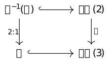
For any of the three rotation groups \(R\), the square records the subgroup and its central double cover. In particular, the Hurwitz-unit model of \(2T\) is this tetrahedral preimage. Its quaternion generators \(i,j,k\) and \((-1+i+j+k)/2\) preserve the 4 imaginary vectors \((1,1,1)\), \((1,-1,-1)\), \((-1,1,-1)\), \((-1,-1,1)\): the first generators change two coordinate signs, and the last cyclically permutes coordinates. Its 24 elements therefore exhaust the preimage. This identifies the group used in the finite spinor gauge example.
TauCeti's
Quaternion.unitaryEquivSpecialUnitaryGroup
formalizes precisely the group equivalence between unit Hamilton
quaternions and \(SU(2)\), using the displayed matrix map. This
correspondence does not assert the \(SO(3)\) quotient or the three
binary subgroup identifications; those have their separate arguments
above. A finite subgroup supplies an available group action, not a
physical interpretation of that action.
Definition 9. A representation datum for a field [fdip-007H]AGENTDRAFTED
- November 1, 2026
Definition 9. A representation datum for a field [fdip-007H]AGENTDRAFTED
- November 1, 2026
A representation datum specifies a finite discrete or compact Hausdorff group \(G\), a scalar field \(\mathbb K\in \{\mathbb R,\mathbb C\}\), a finite-dimensional fiber \(F\) over \(\mathbb K\), a continuous representation \(\rho :G\to GL_{\mathbb K}(F)\), and a separately chosen action \(\alpha :G\to \operatorname {Aut}(X)\) on the finite substrate \(X\). The substrate automorphisms preserve the graph, weights and any supplied oriented cell data, with orientation changes interpreted by the established inverse-transport convention. One must also specify a positive invariant real or Hermitian inner product on \(F\). The field itself is a map \(\phi :V\to F\).
An invariant inner product always exists for these groups. From any positive inner product \(h_0\), define \[h(v,w)=\int _G h_0(\rho (g)v,\rho (g)w)\,d\mu _G(g).\] The normalized Haar measure makes this invariant by a change of variable. The integral is finite by compactness, and \(h(v,v)>0\) for \(v\ne 0\), since \(\rho (g)v\ne 0\) for every \(g\). This proves existence of an invariant metric; it does not make that metric a canonical choice. A selected metric remains part of the background data.
The global action associated to the datum is \[(g\cdot \phi )(v)=\rho (g)\phi (\alpha (g)^{-1}v).\] The two actions have different roles. For a purely internal group, \(\alpha \) is trivial: the group acts on values without moving vertices. A local gauge transformation instead assigns an element \(g_v\) independently at each vertex and transforms links by \(U_e\mapsto g_{h(e)}U_eg_{s(e)}^{-1}\). It fixes the substrate; a global substrate action \(\alpha \) cannot simply be applied independently at each vertex.
If a field has an additional spin space \(S\), an internal action on \(S\otimes F\) is \(1_S\otimes \rho (g)\). Clifford operators \(\gamma _j\otimes 1_F\) then commute with that action because they act on different factors. An identification of internal and spin symmetries, or an action moving the substrate, needs extra compatible data; it is not implied by the abstract group name or by an inclusion in \(SU(2)\).
Example 10. Two fibers for binary tetrahedral symmetry [fdip-007K]AGENTDRAFTED
- November 1, 2026
Example 10. Two fibers for binary tetrahedral symmetry [fdip-007K]AGENTDRAFTED
- November 1, 2026
Take the binary tetrahedral group and a fixed finite substrate, with trivial substrate action in the representation datum. Its spinor datum uses \(\mathbb K=\mathbb C\), \(F=\mathbb C^2\) with its standard Hermitian metric, and the inclusion \(2T\subset SU(2)\). Its rotation datum uses \(\mathbb K=\mathbb R\), \(F=\mathbb R^3\) with its Euclidean metric, and the representation obtained through \(\pi :SU(2)\to SO(3)\).
The latter kills \(\{1,-1\}\), while the former is faithful. Thus these choices define different fibers and observables even though the abstract group and the substrate are the same. The spinor Wilson calculation uses the former. A choice of \(G\) alone would not select that representation.